MODELS FOR PEDESTRIAN TRAJECTORY PREDICTION AND NAVIGATION IN DYNAMIC ENVIRONMENTS
A Thesis presented to
the Faculty of California Polytechnic State University, San Luis Obispo
In Partial Fulfillment
of the Requirements for the Degree Master of Science in Computer Science
by Jeremy Kerfs
c 2017 Jeremy Kerfs
COMMITTEE MEMBERSHIP
TITLE: Models for Pedestrian Trajectory Predic-tion and NavigaPredic-tion in Dynamic Environ-ments
AUTHOR: Jeremy Kerfs
DATE SUBMITTED: May 2017
COMMITTEE CHAIR: Professor John Seng, Ph.D. Department of Computer Science
COMMITTEE MEMBER: Professor Franz Kurfess, Ph.D. Department of Computer Science
COMMITTEE MEMBER: Associate Professor Lubomir Stanchev, Ph.D. Department of Computer Science
ABSTRACT
Models for Pedestrian Trajectory Prediction and Navigation in Dynamic Environments
Jeremy Kerfs
Robots are increasingly taking on roles alongside humans. Before robots can ac-complish their tasks in dynamic environments, they must be able to navigate while avoiding collisions with pedestrians or other robots. Humans are able to move through crowds by anticipating the movements of other pedestrians and how their actions will influence others; developing a method for predicting pedestrian trajectories is a critical component of a robust robot navigation system. A current state-of-the-art approach for predicting pedestrian trajectories is Social-LSTM, which is a recurrent neural network that incorporates information about neighboring pedestrians to learn how people move cooperatively around each other. This thesis extends that model to out-put parameters for a multimodal distribution, which better captures the uncertainty inherent in pedestrian movements. Additionally, four novel architectures for repre-senting neighboring pedestrians are proposed; these models are more general than current trajectory prediction systems. In both simulations and real-world datasets, the multimodal extension significantly increases the accuracy of trajectory prediction. One of the new neighbor representation architectures achieves state-of-the-art results while reducing the number of both parameters and hyper-parameters compared to existing solutions. Two techniques for incorporating the trajectory predictions into a planning system are also developed and evaluated on a real-world dataset. Both techniques plan routes that include fewer near-collisions than algorithms that do not use trajectory predictions. Finally, a Python library for Agent-Based-Modeling and crowd simulation is presented to aid in future research.
ACKNOWLEDGMENTS
There are few open-source tools or methods for trajectory prediction, but Anirudh Vemula shared his Tensorflow implementation of Social-LSTM on Github. His well-written code served as a reference for my own implementation, and I appreciate his contribution to the open-source community and aid in developing this thesis. The communities behind Edward, Mesa, and OpenMVG projects were immensely helpful during my research.
The donors of the Loyal Order of Propeller Heads (LOOP) were instrumental in mentoring me and supporting me throughout my time at Cal Poly. Without them, I would not have attended Cal Poly and would not have enjoyed the opportunities that came from my time at Cal Poly. I am especially indebted to Dr. Hartung for his infectious enthusiasm for for Cal Poly Engineering and its students. His unwaivering dedication to the other LOOP scholars and I motivated us to excel inside and outside the classroom.
Dr. Liu advised my Capstone project and introduced me to the exciting world of agricultural robotics. I thoroughly enjoyed our time out in the fields, seeing what robots can offer the argicultural industry. I am grateful for his support and guidance throughout our research projects.
This thesis would not have been possible without my advisor Dr. Seng. I began this project while he was on sabbatical teaching on the other side of the country, but he nonetheless made time to discuss my progress each week. His passion for robotics kept me motivated; I am thankful for his advice and suggestions throughout the project.
My parents were an endless source of encouragement and support. I am immensely grateful for their guidance and patience.
TABLE OF CONTENTS Page LIST OF TABLES . . . ix LIST OF FIGURES . . . x CHAPTER 1 Introduction . . . 1
1.1 Pedestrian Trajectory Prediction . . . 2
1.2 Navigation in Dynamic Environments . . . 4
1.3 Contributions . . . 5
2 Background . . . 7
2.1 Autonomous Mobile Robots . . . 7
2.1.1 Human-Robot Interaction . . . 7
2.1.2 Sensing and Perception . . . 9
2.2 Neural Networks . . . 10
2.2.1 Recurrent Neural Networks . . . 12
2.2.2 Mixture Density Networks . . . 15
2.2.3 Autoencoders . . . 16
2.3 Navigation . . . 19
3 Related Work . . . 23
3.1 Navigation and Trajectory Prediction . . . 23
3.1.1 Goals of Navigation . . . 23
3.1.2 Reinforcement Learning . . . 24
3.1.3 Probabilistic Models . . . 26
3.1.3.1 Interacting Gaussian Processes . . . 26
3.1.3.2 Obstacle Maps . . . 27
3.1.4 Social Forces . . . 28
3.1.4.1 Learning Social Etiquette . . . 29
3.1.5 Neural Networks . . . 30
3.1.5.1 Social-LSTM . . . 30
3.2 Deep Representations . . . 35
3.2.1 Attention in Neural Networks . . . 35
3.2.1.1 Soft and Hard Attention . . . 36
3.2.1.2 Spatial and Temporal Attention . . . 37
3.2.2 Hierarchical Recurrent Neural Networks . . . 38
3.2.2.1 Spatial Temporal Learning . . . 38
3.2.2.2 Natural Language Processing . . . 39
4 Design . . . 40
4.1 Multimodal Predictions . . . 40
4.1.1 Prediction Examples . . . 45
4.2 Neighbor Representations . . . 47
4.2.1 Occupancy Grid (OCC) . . . 51
4.2.2 Hierarchical LSTM (HIER) . . . 53
4.2.3 Spatial Attention (SATTN) . . . 56
4.2.4 Neighbor Attention (NATTN) . . . 58
4.2.5 Representation Summary . . . 61
4.3 Planning in Dynamic Environments . . . 64
4.3.1 Dynamic Horizon A* . . . 64
4.3.2 Tree Search . . . 68
5 Implementation . . . 74
5.1 Simulations . . . 74
5.1.1 Hardware and Software . . . 77
5.2 Reducing Overfitting . . . 78
5.2.1 Data Augmentation . . . 78
5.2.2 Dropout . . . 79
5.2.3 Weight Regularization . . . 80
5.2.4 Early-Stopping . . . 81
5.3 Pre-training with Autoencoders . . . 82
6 Results . . . 85
6.1 Trajectory Prediction . . . 85
6.1.1 Simulations . . . 86
6.1.2.1 Limitations . . . 93
6.2 Destination Prediction . . . 94
6.3 Planning in Dynamic Environments . . . 98
7 Argil - Crowd Simulation . . . 106
7.1 Design . . . 106
7.1.1 Model Definition . . . 107
7.1.2 Visualization and Data Output . . . 109
7.2 Comparison . . . 112
7.3 Performance . . . 113
8 Future Work . . . 116
8.1 Trajectory Prediction . . . 116
8.2 Planning in Dynamic Environments . . . 118
8.3 Crowd Simulation and Modeling . . . 119
9 Conclusion . . . 122
9.1 Recommendations . . . 126
LIST OF TABLES
Table Page
2.1 Common Sensors for Autonomous Mobile Robots . . . 9
4.1 Number of Learned Parameters for Architectures . . . 64
6.1 Results for Intersection Simulation . . . 88
6.2 Results for UCY Dataset . . . 92
6.3 Destination Prediction Results . . . 96
6.4 Results of Path Planning . . . 100
LIST OF FIGURES
Figure Page
2.1 LSTM Neuron . . . 14
2.2 Simple Mixture Density Network . . . 15
2.3 Autoencoder . . . 17
2.4 Costmap . . . 20
3.1 Sample Scenario . . . 31
3.2 Core Social-LSTM Architecture . . . 32
3.3 Neighbor and Coordinate Representations for Social-LSTM . . . 33
4.1 Viable collision avoidance routes . . . 41
4.2 Basic Trajectory Prediction . . . 46
4.3 Multimodal Trajectory Prediction . . . 47
4.4 Structure of Personal Space . . . 49
4.5 Occupancy Grid Architecture (OCC) . . . 52
4.6 Hierarchical LSTM Architecture . . . 54
4.7 Spatial Attention Architecture . . . 58
4.8 Spatial Attention Architecture . . . 60
4.9 Structure of Social Tensor . . . 61
4.10 Relevant Neighbor Regions for Architectures . . . 63
4.11 Dynamic Horizon A* at Each Timestep . . . 67
4.12 Tree Search at Each Timestep . . . 73
5.1 Representative Sequence from Hallway Simulation . . . 75
5.2 Representative Sequence from Fork Simulation . . . 76
5.3 Data Augmentation . . . 79
5.4 Autoencoding Architecture for Trajectories . . . 82
5.5 Effect of Pretraining on Learning . . . 83
6.1 Representative Sequence from Intersection Simulation . . . 87
6.3 Sample Frames of UCY Dataset[32] . . . 90
6.4 UCY Results . . . 93
6.5 Qualitative Destination Prediction Results . . . 97
6.6 Sample Routes 1 . . . 102
6.7 Sample Routes 2 . . . 103
6.8 Overly Cautious Behavior . . . 104
6.9 Failure to Walk Side-by-Side . . . 105
7.1 Initialization of Simulation . . . 108
7.2 Observations while running Simulation . . . 110
7.3 Argil Visualization in Jupyter Notebook . . . 111
7.4 Effect of Number of Agents on Performance . . . 115
Chapter 1 INTRODUCTION
Robots have become pervasive in a variety of industries and applications. They are able to complete military operations, clean homes, fight forest fires, and transport machinery. Previously, robots were confined to predictable situations like assembly lines where the robots would perform rote tasks. However, now robots navigate complex and dynamic worlds and must adjust their behavior in real-time to changing conditions. Robots must learn from other humans and robots in order to perform well in these situations. Additionally, robots must accurately perceive their surroundings and rapidly process this information to make informed decisions and complete their tasks.
Mobile robots are robots that can move. Roomba vacuum cleaners, self-driving vehicles, and bomb-disposal robots are all mobile robots. Mobile robots are especially challenging to develop and deploy because engineers must carefully specify how the robot should react to all of the conditions that it could encounter while moving. Three core tasks of all mobile robots are mapping, localization, and navigation. Mapping is the process of learning and describing the robot’s environment. Localization is the process of determining where the robot currently is located. Navigation combines knowledge of the environment (map) and the robot’s position within the environment (location) to plan routes from the current location of the robot to specific waypoints (destinations). Mobile robots should then be able to execute these routes by moving through the environment. The quality of a route may depend on how short it is, the amount of hazards on the route, and the impact that the route will have on other agents. Humans are adept at considering all of the aspects of a route and formulating the best option, so there is potential for robots to learn this behavior from humans,
but it comes with great challenges.
A common approach in modern robotics research is to train robots to behave like humans. If mobile robots can navigate and interact with humans in a pleasant, non-intrusive, and non-threatening way, then the robots will be better able to carry out mundane tasks that humans would otherwise be required to perform. Autonomous cars are an application of robotics where it is especially critical that the robot (car) act in ways that other humans would expect. Even though autonomous cars have the capability to dart in between cars with just inches of space between the bumpers, humans would be frightened with these close encounters and might react poorly, causing accidents. Instead, autonomous cars are designed to drive and respect the space of other cars the way human drivers do. The same principles can be applied to other mobile robots. The focus of this thesis will be on pedestrian environments. In some ways, robot navigation in pedestrian environments involves more uncertainty than autonomous driving due to the more predictable structure of the driving envi-ronment. In driving scenarios, the lanes, signs, and right-of-way rules all constrain the possible movements of a car and other cars around it, while pedestrian environ-ments like shopping malls, schools, and airports have limited rules, and the behavior of agents within these environments is much less predictable. Yet, pedestrians still follow implicit rules and respond in predictable ways to outside events.
1.1 Pedestrian Trajectory Prediction
Before attempting to navigate a crowded area, humans predict the state of the envi-ronment several steps ahead. They anticipate potential dangers or collisions before they occur. They detect subtle behaviors of others to understand how people re-act and behave around one another. Once they have assessed the situation, humans use their predictions to formulate a desirable route. This thesis will investigate how
robots can achieve the forecasting ability of humans in pedestrian environments. This forecasting is an essential component for any robot that must cooperatively interact with people.
While humans learn many tasks and behaviors through experiential learning (trial-and-error), moving in crowded environments is learned through watching others’ be-havior. It would be infeasible and ethically dubious to train robots to move in dynamic pedestrian environments through trial-and-error since the learning process would cer-tainly include many collisions. Rather, the preferred approach is to build a system that can forecast the positions of pedestrians in the future. This prediction system can then be utilized to plan appropriate routes and avoid collisions.
Humans make decisions based on complex rules and intuitions about their envi-ronment that they have learned over many years. It is infeasible to fully enumerate and encode the rules that govern human behaviors into an algorithm for predicting human movements. The influences of human movements are varied, and attempts to codify them would likely omit important edge cases (uncommon situations). One way to overcome this challenge is to build a system that can learn these rules through examples. Machine learning is the study of algorithms that learn to make predictions using data. In the case of trajectory prediction, this data could be videos of people walking in public areas.
Since humans are so adept at learning to predict pedestrian movements, a logical machine learning algorithm for estimating trajectories is a system that mimics human learning. While the neuroscience connection is somewhat tenuous, neural networks are a machine learning algorithm that has a basis in the neural pathways of animal brains. Neural networks are a widely successful tool for many domains where systems are taught to recognize and perform tasks at (or above) human-level performance. Recently, neural networks were applied to predicting human trajectories in dynamic
environments. This thesis will extend and improve those results in order to develop a solution for estimating the movements of pedestrians.
1.2 Navigation in Dynamic Environments
After building a model for predicting the trajectories of pedestrians, the next step is to construct a navigation algorithm that can incorporate these predictions. Such a navigation system must be able to effectively plan routes that avoid collisions (or uncomfortably close interactions) between a robot and other robots or pedestrians. Effectively, the trajectory prediction system provides foresight into where people are going, and this foresight can be used to plan better routes. Of course, there are many other factors that go into planning besides the forecasts of pedestrian behavior. A planning algorithm should be able to take into account the kinematic constraints of the robot (what kinds of movements are possible), environmental features (terrain and objects), and the goals of the robot (e.g. minimizing path length or perturbations of other agents).
Planning, and more specifically path planning, is a rich area of research with many algorithms designed for specific use-cases. In this thesis, two of these common approaches are modified and applied to planning robot paths in dynamic environments using the predictions of pedestrian trajectories from the neural network models. The first approach extends A* - a search algorithm for finding shortest paths that uses heuristics to find optimal paths while minimizing the exploration of routes that are unlikely to be optimal. The second approach is a tree search that calculates the sequence of movements that bring the robot closest to its destination. In this work, these two methods are applied to the dynamic navigation task and are evaluated on real-world datasets.
1.3 Contributions
This thesis will focus on the use of neural networks for predicting trajectories and their application to planning in dynamic environments. It makes the following con-tributions:
• Applies Mixture Density Networks for trajectory prediction,
• Designs four novel neural network architectures for representing pedestrian in-teractions,
• Constructs two planning approaches for navigating in dynamic environments, and
• Builds a new library, called Argil, for Agent-Based-Modeling and crowd simu-lation
Mixture Density Networks allow for a neural network to more accurately represent the uncertainty of an agent’s position than previous techniques. The previous state-of-the-art approach used a unimodal distribution for trajectory prediction, which is unable to capture the multiple likely paths that pedestrians can take. The novel neural network architectures for pedestrian trajectory prediction achieve comparable results to state-of-the-art models, but they have fewer hyper-parameters to tune than existing solutions. These neural network architectures, to the best of our knowledge, are the first models for trajectory prediction that make no assumptions about which nearby pedestrians are likely to influence the movements of another pedestrian. To demonstrate the practical application of the trajectory prediction models, two path planning algorithms are adapted to dynamic environments by incorporating predic-tions from the neural network model. Argil, the new Agent-Based-Modeling library,
for model design, visualization, and data output. Argil is the first Python library for pedestrian simulations; it allows developers to more rapidly iterate their simulations than existing alternatives.
This thesis document will first describe the relevant context for this project in Chapter 2. Then the other methods and techniques for trajectory prediction and navigation in dynamic environments will be discussed in Chapter 3. Next, in Chapter 4, the architecture and core attributes of the new neural network solutions will be presented along with the path planning techniques. In Chapter 5, the construction of the system will be explained. The experimentation and testing will be discussed in Chapter 6. Chapter 7 presents the Argil simulation library that was used for building and debugging the models that are presented in the thesis. The opportunities for continued research will be presented in Chapter 8, and the significance of this research will be assessed in Chapter 9.
Chapter 2 BACKGROUND
Autonomous robot navigation has a rich history of research with many advances occurring in the past decade. Work in machine learning has become increasingly rel-evant for robotic systems; this thesis relies heavily on the machine learning technique called neural networks. This chapter will begin with an explanation of autonomous robots and perception, followed by a survey of relevant neural network concepts. The last section will discuss navigation algorithms.
2.1 Autonomous Mobile Robots
Autonomous robots operate without explicit human control. Semi-autonomous robots receive intermittent instructions from humans but often function independently. There are number of key capabilities that mobile autonomous robots must posses in order to be successful. The first priority is that the robots are safe - they do not damage themselves, objects, people, or animals. Once the robots are deemed safe, they must be able to cooperate and work alongside humans in a predictable and human-friendly manner. If the robot is mobile then it must be able to determine its location, under-stand its environment, and navigate to its destinations. This section will describe the current state of autonomous robots and how they interact with humans.
2.1.1 Human-Robot Interaction
Human-Robot interaction is the study of how humans and robots exchange infor-mation and work together or adversarially. It is often considered a sub-discipline of human-computer interaction, although there are number of key distinctions. The
nature of robots makes the interaction between them and humans especially critical because robots have the capacity to directly inflict physical harm. Humans are also much less familiar with robots than they are with computers, so it is more difficult to predict how humans will react. Another complication with human-robot interaction is the delayed response; since robots typically respond with physical actuation, hu-mans may have to wait longer to receive feedback instead of the immediate feedback that they receive from a computer screen.
A key aspect of Human-Robot Interaction that is important for this thesis is the communication between humans and robots. Since humans rarely direct robots, they are not well-versed in the capabilities and limitations of robots. Most robot systems must be operated by experts who program the robot explicitly by setting navigational waypoints or precise arm movements. These modes of interaction are acceptable for controlled environments, but their performance deteriorates in complex, dynamic settings. Researchers have attempted to build more robust systems for handling human-robot interaction; notably researchers from Carnegie Mellon developed the The Human Robot Interaction Operating System[13], which attempts to rigorously define how humans and robots should effectively communicate. There are a variety of ways that humans can communicate with robots - visually, orally, and cognitively[8] among others.
It is generally desirable for robots to communicate with humans in approximately the same way that humans communicate with each other. Human-to-human commu-nication involves conscious choices (like speech) and subconscious actions (like body language). This paper focuses on the way actions convey information. When humans are walking in a crowded environment, they communicate with other pedestrians by signaling their intent through actions. Moving purposefully forwards indicates that the person wants to continue forwards, while pausing or slowing down indicates that the person is willing to yield or is preparing to stop or turn. If a person chooses to
Table 2.1: Common Sensors for Autonomous Mobile Robots Sensor Method
Lidar laser beam Sonar sound waves Cameras visible light
Radar radio waves
take a circuitous route, other pedestrians may conclude that the person was avoiding a dangerous or unpleasant situation. For robots to navigate and interact in these crowded environments, they must be able to understand and respond to these subtle cues and provide the same cues.
2.1.2 Sensing and Perception
In order for autonomous robots to safely operate and complete tasks; robots must be equipped with sensors for perceiving the world. Additionally, robots must have the capacity to analyze the sensor inputs and determine appropriate responses. Sensors and computing resources can be located on the robot platform itself or externally. The quality of the sensors and the computational resources are key limitations for robots. Table 2.1 shows the most common sensors found on autonomous mobile robots. It is critical to consider the available sensors because the information provided by sensors often differs dramatically from the information available to humans from their senses. The designs produced in this thesis could be implemented on any robot platform that has the capacity to identify and track other agents. Cameras and Lidar would be especially well-suited for navigation in dynamic environments because they can provide frequent updates (more than 30 times per second), and they typically produce dense representations of the environment. The raw data from these sensors must be
processed to estimate the position of other other agents in the scene.
2.2 Neural Networks
Artificial Neural Networks are models for learning complex, often non-linear functions. They can be used to perform classification, regression, and clustering. The neural connections and structure of brains inspired the development of neural networks. The concept was developed in the 1940s, but neural networks lost popularity in the 1990s as other machine learning techniques proved more successful. With massive increases in computing power and vast amounts of data, neural networks achieved renewed popularity in the 2000s. In the late 2000s and 2010s, neural network solutions achieved state-of-the-art results in diverse fields including image classification[29][49], machine translation[57], and speech recognition[3].
Neural networks are composed of neurons; the neurons have weights that are adjusted through training to produce the desired outcomes based on the inputs. These neurons are connected to other neurons; each neuron will apply a function to the inputs that it receives from other neurons to produce a result. Neurons are grouped into layers based on which neurons they are connected to and what function they apply to inputs. There is a tremendous variety of neuron functions and ways of connecting neurons, but a few designs have proved to be the most useful. Generally the level of neurons is not meaningful in large, modern neural networks because the interconnections between neurons is complex. Rather, most neural networks are described by their layers. Layers are groupings of neurons that all perform equivalent operations.
The most common and simplest layer for neural networks is the fully-connected layer. Each neuron in a fully-connected layer receives the output from every neuron in the previous layer. The neurons will then apply a specific weight to the value of
each input and then sum the weighted values. Typically a sigmoid or relu (rectified linear activation) is then applied to the sum in order to add non-linearity to the network. The final value computed in each neuron is the input to neurons in the next layer. The weight that each neuron applies to each input is modified during training. A Feed-Forward Network is a neural network where there are no loops (the outputs only propagate forward through the network). A simple fully-connected layer can be written using matrix multiplication and vector addition as shown in Equation ?? where X is the inputs from the previous layer. X is a column vector with m values where m is the number of neurons in the previous layer. W is the weight matrix with dimensions l by m where l is the number of neurons in next layer. b is a bias column vector with l values. f is an activation function like a relu, sigmoid, or hyperbolic tangent. o is the values of the neurons in the next layer. The first layer in a neural network is generally the input features, and so there are no parameters in this first layer.
o=f(W X+b) (2.1)
Neural networks are typically trained through a process called Backpropagation. For classification tasks (where the neural network outputs the class of the input), the network is provided with inputs and the correct class of the input. For regression tasks (the output is a continuous value), the network is also provided with input features and the actual value of the features. The network is evaluated with the each input, and the output of the neural network is compared to the correct output. Then the weights are updated based on the error of the network. Backpropagation calculates the errors of each neuron based on the error of the entire network. These errors are calculated by sequentially propagating errors backwards through the network in the
derivative of the neuron functions to determine the errors of the neurons. The weights are updated based on the contribution to the error using an optimization algorithm; a basic optimizer is Stochastic Gradient Descent (SGD). However, recently more advanced variations of SGD have reached common usage. During training, the error of the network is evaluated on a subset of training data and then the optimization algorithm is applied to make small updates to the weights in order to minimize the loss function (a quantitative assessment of neural network performance). This process is continued for a specified amount of time or once the loss function ceases to decrease.
2.2.1 Recurrent Neural Networks
While Feed-Forward neural networks have no loops, recurrent neural networks (RNNs) allow the output of neurons to be fed back into the same neuron or previous neurons. This is an important property because it enables the neural network to perform pre-dictions based on the current input and the previous state of the network. RNNs are essential in many domains that involve time series data like translation, natural lan-guage processing, and video prediction. The additional capabilities of RNNs come at the expense of more difficult training. Backpropogation can still be used, but it must be modified to handle the loops in the network. The common extension to Backpro-pogation is called BackproBackpro-pogation-Through-Time (BTT), which involves unrolling the recurrent layers (duplicating the neurons) to create a feed-forward network for a certain number of steps. The gradients can then be computed on this network, and the errors are propagated to the unrolled neurons. The weights are updated to adjust the parameters of the original recurrent neurons. Although BTT is an elegant solution to training RNNs, it often requires significant memory when the network must be unrolled for many steps.
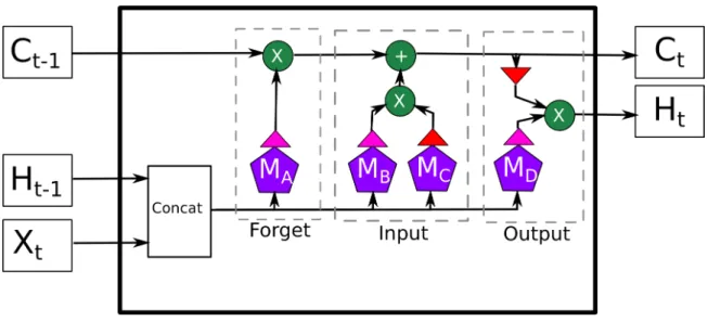
with the new input data. The downside of this approach is that it becomes difficult for a neuron to retain information for many steps. One solution to this is the Long Short-Term-Memory (LSTM) cell [23]. The basic version of an LSTM cell is shown in Figure 2.1. There are three gates in an LSTM (forget, input, and output). The forget gate (in the dashed box on the left) concatenates the previous cell state with the input and then multiplies the concatenation by a weight matrix and adds a bias vector; the result is fed into a sigmoid activation function. The output of this process is multiplied by the previous hidden state. All locations where the forget gate outputs a low value are lowered in the hidden state - causing the network to ”forget” the values. The input gate has two parts. The first part applies the sigmoid activation to the concatenation of the input and previous cell state after multiplying the concatenated inputs by a weight matrix and adding a bias vector. The second part of the input gate, applies the hyperbolic tangent function same concatenation after multiplying the concatenated inputs by a different weight matrix and adding a different bias vector. The two parts of the input gate are multiplied together (element-wise) and added to the hidden state - essentially incorporating new information in the cell. The output gate also has two compoents. The first component is the hyperbolic tangent applied to the updated hidden state. The next component is sigmoid function applied to the the concatenation of the input and previous hidden state after multiplication by another weight matrix and the addition of a final bias vector. These two components are multiplied together element-wise to produce the next hidden state and output of the cell.
In Figure 2.1, the pink triangles denote the sigmoid activation function, while the red triangles are the hyperbolic tangent activation function. The purple hexagons are multiplications of the input by a weight vector and the addition of a bias vector (similar to a fully-connected layer). The Mi symbol denotes the parameters used in
Figure 2.1: LSTM Neuron
and the green + is the addition of the vectors. The same structure is expressed in Equation ??. κ represents the matrix multiplication with a weight matrix, addition of a bias vector, and the application of the sigmoid activation functions. ρ similarly represents the multiplication with a weight matrix and addition of a bias vector, but the activation function is the hyperbolic tangent.
zt =concat(ht−1, xt) at =κ(zt;Ma) bt =κ(zt;Mb) ct =ρ(zt;Mc) dt =κ(zt;Md) ct = (ct−1·at) + (bt·ct) ht =ρ(ct)·dt (2.2)
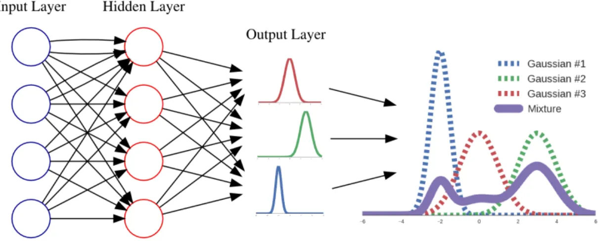
Figure 2.2: Simple Mixture Density Network
2.2.2 Mixture Density Networks
Many of the most successful applications of neural networks are for predicting cat-egorical values like the object in an image or the word that was uttered. However, neural networks have also been used for regression problems where the output is a continuous value. For example, neural networks have been used to predict stock prices [26][31]. There are some situations that arise in regression problems where the output is best approximated with a multi-model distribution. Using stocks as an example, it would be beneficial for a neural network to express the hypothesis that the stock price will go down by 1% with 80% certainty or go up by 2% with 20% confidence, but it is unlikely for it to stay the same. In order for a neural network to produce such a prediction, the model would have to have several output neurons along with weights denoting the certainty of each prediction.
Mixture Density Networks are a general framework for making multimodal pre-dictions. They were introduced by Bishop in 1994 with a demonstration of their application to inverse robot kinematics[6]. A Mixture Density Network outputs the parameters of a mixture of probability distributions along with weights for combining
the component distributions. Typically, the composite distributions are Gaussians, but it is possible to use other distributions. A simple example of a Mixture Density Network is shown in Figure 2.2. The network accepts inputs and transforms the inputs through several layers into the parameters of a mixture distribution.
Mixture Density Networks are closely related to Mixture Models, which are ubiq-uitous in Bayesian statistics. In probabilistic modeling, Mixture Models are used to infer the latent substructure of a larger group. Both Mixture Models and Mixture Density Networks use a composition of distributions to represent a concept. Mixture Models are used to represent the properties of a population by learning the compo-nent distributions directly from the data (typically using Expectation Maximization or Markov Chain Monte Carlo techniques). Mixture Density Networks represent a prediction by learning the component distributions from a neural network applied to inputs.
Mixture Density Networks have be incorporated into models for a variety of ap-plications. Speech and acoustics are good candidates for Mixture Density Networks because the frequencies can be expressed as a mixtures of Gaussians [44][59]. RNADE (real-valued neural autoregressive density-estimator) extends Mixture Density Net-works by sharing distribution parameters and making subsequent distributions con-ditional on previous ones [54]. RNADE is not considered in this work, but it could be a candidate for future work. Alex Graves developed a Mixture Density Network to generate handwriting samples by representing the location of the pen with a mixture of Bivariate Gaussians [17].
2.2.3 Autoencoders
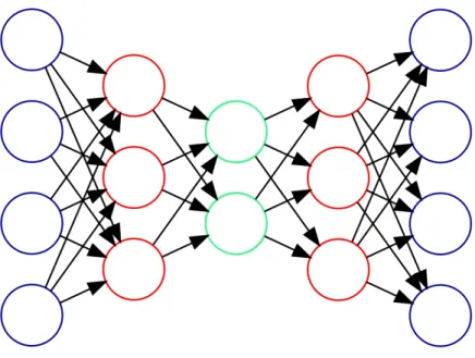
Autoencoders are a type of neural network used for unsupervised learning. The basic autoencoder encodes its inputs into a latent representation and then decodes the
la-Figure 2.3: Autoencoder
tent representation to approximate the inputs. The network is trained by minimizing the difference between the output of the network and the input. Both the encoding and decoding layers can be deep neural networks. Figure 2.3 illustrates a simple au-toencoder where the blue nodes on the left are the original input and the blue nodes on the right are the reconstructed input. The red nodes are hidden layers, and the green nodes are the latent representation.
There are two main considerations when designing autoencoders - the encod-ing/decoding structure and the latent representation. Typically, the encoding and decoding neural networks are symmetric. The latent representation must be chosen carefully. If the latent representation has a higher dimension than the input dimen-sions then the autoencoder risks simply memorizing the input data and returning it without learning any interesting structure. To avoid this, researchers have developed several strategies. The most basic solution is to use a small latent layer (like the one shown in Figure 2.3) that has many fewer units than the input dimensions. An alternative is to apply regularization to the activations of the neurons in the latent
representation.
One form of regularization is the sparsity constraint. The sparsity constraint adds a penalty for all of the neurons in the latent layer that are activated (have a high output value). The result of the sparsity constraint is that only a few neurons will be active in the latent layer, which forces the autoencoder to learn the underlying structure of the input data that differentiates each input from the rest. Care must be taken when training an autoencoder with a sparsity constraint to ensure that the sparsity penalty is not too high that no neurons are activated nor too low so that nearly all neurons activate.
Another more complex form of regularization of the latent representation is the Variational Autoencoder (VAE). A VAE regularizes the latent representation by forc-ing activations of the neurons in the latent layer to not significantly deviate from a Gaussian distribution. VAEs tend to produce dense representations where each neu-ron in the latent layer is activated, but the values are constrained to a small range. In a VAE, the encoding layer outputs a list of means and standard deviations (the number of means/standard deviations is the latent layer size). Then a sample is taken from each Guassian distribution defined by the means and standard deviations. These samples become the latent representation of the input. The samples are then passed to the decoding network to reconstruct the input. The loss for a VAE is the reconstruction cost (the same as all other autoencoders) and the Kullbach-Leibler Divergence between the Gaussians defined by the encoder and a predefined Gaussian (typically with a mean of 0 and a standard deviation of 1). The Kullbach-Leibler Di-vergence (KL-D) is a continuous value that describes how different two distributions are from each other. The formula for the continuous version of KL-D is shown below:
DKL(P|Q) =
Z −∞
−∞
p(x)·log(p(x) q(x))
It is important to note that KL-D is not symmetric because DKL(P|Q) does not
necessarily equal DKL(Q|P).
2.3 Navigation
Navigation is the process of determining the steps necessary to get from one place to another. Typically, the goal of navigation is to minimize the cost of movement to a destination. The cost of a route to the destination can include the length of time required, the amount of energy consumed, or the probability of a collision. Prior to performing navigation, the areas of the environment that are safe to traverse must be determined. Additionally, the criteria for selecting a route must be defined. These criteria can vary, but typically in the context of robotics, the shortest route that avoids damage to the robot or the environment is chosen. Navigation can occur at many levels of granularity. For example, a traveler performs navigation by planning to drive to the train station and take a train to the beach. Then the traveler will use maps to plan the optimal sequence of roads to take in order to reach the train station. While driving, the traveler will actively navigate around obstructions in the road, possibly taking detours in order to avoid accidents. This example shows how navigation can be performed at a high-level (drive then ride the train) or at a lower-level (driving wide around an obstruction). Humans are able to seamlessly switch between levels of planning when necessary, but teaching robots to effectively navigate is a non-trivial endeavor. Robots must learn or be programmed to predict human actions, emulate human activity, and respond appropriately to unforeseen events like natural disasters or malicious behavior.
An excellent example of constructing a robot system for navigation is the Naviga-tion Stack in the Robot OperaNaviga-tion System (ROS)[43]. ROS is a library and framework that is commonly used for robotics. ROS provides a modular way of defining
com-Figure 2.4: Costmap
ponents that accomplish specific tasks for the robot. Researchers, corporations, and hobbyists share their components (called Nodes) with the open source community. The purpose of ROS is to have a unified way of orchestrating all of the various be-haviors and functionality of robots. The ROS Navigation Stack is a well-documented and thoughtfully-designed system for route planning that has been implemented for many robot platforms. The following paragraphs consider the ROS Navigation Stack as a case study in how navigation systems can be built and deployed on autonomous robot platforms. There are many other solutions for navigation systems, but they all share many of the same design choices, and it is therefore necessary to only study one of them.
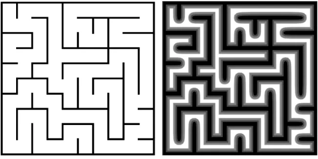
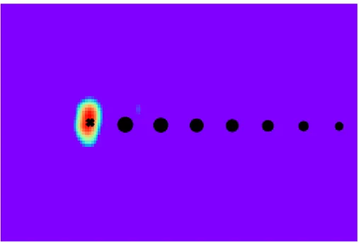
Before a robot can navigate and plan paths, the robot must have a map of the environment and know its location in the environment. In ROS, a map of the en-vironment can be produced by the robot while it explores the enen-vironment, or an existing map can be used. The basic map defines what regions are safe and which are not. In ROS, these maps are costmaps. Figure 2.4 is an example of a costmap
constructed from a maze layout. The light regions of the map are navigable while the darker regions are considered dangerous or impossible to move through. Notice that the original map on the left shows the hard walls of the maze, while the map on the right has fuzzy boundaries around the walls. The map on the right is generally preferable because it demonstrates that the robot should not only avoid running into a wall but also avoid close proximity to a wall since the robot may slide or get pushed resulting in a collision. These 2D costmaps can be used for planning.
In ROS, there are global planners and local planners. Global planners use the costmaps and plan a route to the destination that minimizes length of the path while also avoiding dangerous (darker) areas on the map. The basic global planner uses the A* search algorithm. A* is an efficient search method that uses heuristics to focus planning on regions of the map that are more likely to yield optimal routes to the destination. The local planners use the route defined by the global planner and outputs instructions for the robot to ensure that the robot uses its actuators to follow the global plan as closely as possible. A key task for building successful robots is to write a system that correctly balances long-range and short-range planning. In the simplest implementation, neither the local planners nor the global planners consider the movement of other agents. Of course, sensors can detect pedestrians or moving vehicles, but the robot treats these the same as static obstacles. This is a major lim-itation because it means that robots using these navigation tools cannot effectively move in dynamic environments without colliding or being overly cautious and failing to make forward progress. A navigation system that will succeed in dynamic envi-ronments must incorporate knowledge of other agent’s trajectories at both the local and global levels.
While there is tremendous variety in navigation algorithms, there is even greater diversity in map building techniques. Navigation systems will always be limited by
robot to explore an unknown area and construct a map piece-by-piece as it moves around. This requires that the robot estimate its own location and the location of objects around it at the same time. SLAM (Simultaneous Localization and Mapping) is the term that describes this task and the associated solutions for it. One limita-tion of most SLAM algorithms is that they are not robust to moving agents in an environment. For example, if a person walks in front of a robot while it is exploring, it may denote the person as an obstacle in the map even though the person is not a permanent fixture of the environment. While maps should be free of transitory ob-jects and agents, the position and velocity of mobile agents is an essential component of navigation. The task of fusing static maps with information about mobile agents is still an active area of research. This thesis will focus exclusively on the effect of mobile agents on trajectory prediction and applications for navigation, but it is im-portant to consider that real-world navigation must incorporate static and dynamic features.
Chapter 3 RELATED WORK
3.1 Navigation and Trajectory Prediction
Navigation and obstacle-avoidance in dynamic environments is a challenging task for robots. Recently researchers have developed many methods for robot navigation that enable robots to actively avoid collisions and minimize the discomfort of humans while still allowing the robot to reach its destination. Complimentary to navigating in dynamic environments is predicting how other agents will move. Often the tasks of trajectory prediction and navigation are approached together, so this section discusses methods for navigation and trajectory prediction.
3.1.1 Goals of Navigation
The most obvious objective for any navigation technique is to plan a route from one location to another. A navigation algorithm cannot be considered successful if it does not produce a viable path to the destination. However, there are many other considerations when the navigation occurs in a crowded environment. Kruse et al. produced a thorough survey of the criteria for successful robot navigation in the presence of humans [30]. Kruse et al. identified three major categories of evaluation metrics that can be used to determine how well a robot navigates - comfort, naturalness, and sociability. A robot that does not invoke fear, stress, or unease in humans would be comfortable for humans to be around. Robots that navigate, move, and interact like humans are considered natural, while robots that respect cultural/social rules like right-of-way would have a high degree of sociability. These categories are abstract and not amenable to specifying in an algorithm; however, other
researchers have considered quantitative metrics that can measure the success of a robot at navigating a human environment. Many researchers have devised penalties for robots that get too close to a person.
3.1.2 Reinforcement Learning
Reinforcement Learning (RL) is the process of learning from repeated trials. The problem of Reinforcement Learning is typically described a Markov Decision Process (although there are several other variations). A Markov Decision Process (MDP) is defined as a state space, an action space, a probability of going from one state to another conditioned on the action taken, and the rewards that are received for tran-sitioning from each state to another state. For robot navigation, the state space is typically all physical locations that a robot can occupy; the action space is all phys-ical actuations that the robot can perform. The probability of transitioning from one state to another is dependent on the features of the environment and the other agents. Rewards are problem-specific, but typically robots would be rewarded for getting close to their destination and not colliding or interfering with other agents. Inverse Reinforcement Learning (IRL) is the task of learning the reward function for a Markov Decision Process. Several researchers have applied IRL to cooperative naviga-tion. The following paragraphs describe three illustrative examples of reinforcement learning in robot navigation.
Chen et al. used Deep Reinforcement Learning for producing short collision-free paths for multiple agents[9]. Deep Reinforcement Learning is a way of solving RL problems using neural networks to estimate the value of going from one state to another or the value of an action and state pair. Chen et al. only considered simulations, but their results showed that neural networks can learn to incorporate cooperative collision avoidance and constraints to produce efficient and safe paths.
Ziebart et al. used IRL and Bayesian methods to output the log-likelihood of a pedestrian’s next locations [60]. They conducted the experiment using real-world data collected from observing a kitchen. The environment was discretized into a grid, and the cost of visiting each cell was learned conditioned on the distribution over possible destinations. They then planned the path of a robot based on the current map. After planning a step, they simulated the trajectories of other pedestrians and updated the cost of cells based on the likelihood that pedestrians would be hindered by a robot’s presence in that cell. The algorithm lets the developer define the trade-off between efficiency of the robot reaching its destination and the amount of hindrance to pedestrians. The main limitation of the approach is that it does not model the responses of pedestrians to the robot (see the Frozen Robot Problem in the next section). In a realistic scenario, humans move out of each other’s way and are thus likely to also yield to a robot; however, the approach taken by Ziebart et al. does not model this possibility.
Kretzschmar et al. designed a probabilistic framework for robot navigation where the importances of various features on the paths are learned from examples of human movements [28]. Some of the features considered are proximity to obstacles, proximity to other pedestrians, and changes in velocity/acceleration. The authors use Mixture distributions to represent choices between several options (such as passing an obstacle on the right or the left). The work is experimentally validated using a contrived environment where humans were observed for four hours. A strong advantage of the engineered features is that it is possible to interpret the impact of other agents and obstacles in a straightforward, probabilistic way. The downside of the engineered features is that it may not generalize to complex environments.
3.1.3 Probabilistic Models
3.1.3.1 Interacting Gaussian Processes
Trauntman and Krause developed the Interacting Gaussian Process (IGP) model to solve thefrozen robot problem[52]. When a robot is given a destination, but there are people in the way, the robot may be unable to make forward progress and therefore appear ”frozen”. Humans do not experience this problem because they engage in cooperative navigation where humans make room for other humans when they notice that someone intends to move through the crowd.
The IGP model represents the trajectories of agents (humans and robots) as a Gaussian Process. A Gaussian Process is a distribution of functions, where the dis-tribution of values at each step is a Gaussian random variable. In the context of trajectory prediction, each step is a random variable that defines where the agent is likely to be; the Gaussian Process is the distribution over these individual random variables and thus represents a trajectory. Trauntman and Krause developed the theory for IGP using one-dimensional trajectories, but additional Gaussian Processes could be used to model the three dimensions of the Euclidean coordinate space. A Gaussian process is defined by a mean and a covariance function. The distribution for any time step is a function of all previous time steps. A standard Gaussian Process has no way of directly incorporating information from other Gaussian Processes (tra-jectories), so Trautman and Krause introduced a potential function. They multiply the Gaussian Process’ probability density for each timestep of an agent by a potential that shifts the distribution away from the other agents. The resulting distribution can be multimodal, unlike the original Gaussian Process random variables. Trauntman and Krause parameterized the potential based on the minimum distance that is seen between pedestrians.
When predicting the next position of a pedestrian, the Maximum A-Posteriori (MAP) estimate of the position is chosen. The MAP estimate is the mode of the posterior distribution, where the posterior distribution is the result of multiplying the distribution of the step of the Gaussian Process with the potential function. The mode is the single most likely position. Trauntman and Krause advocate the use of importance sampling, which approximates the MAP estimate through multiple samples from the posterior distribution.
IGP is a promising technique because it can represent multimodal distributions and has relatively few parameters. Trauntman and Krause report that reasonable estimates can be computed in less than .1 seconds, so the approach seems to be fast enough for real-world applications. The potential function allows the robot to infer how people will move in order to accommodate it, thus resolving the frozen robot problem. IGP was also validated on a robot in a crowded cafeteria [53]. The major limitation of IGP is that it assumes that robots can move just like humans, and the custom potential function may not be applicable to heterogeneous agents (cars, bikes, etc.) or be able to incorporate long-range influences.
3.1.3.2 Obstacle Maps
Vemula et al. constructed a variation of the IGP model that represented the neighbors of an agent in an occupancy grid [56]. The occupancy grid encodes the locations of other agents relative to the agent whose trajectory is being predicted. The squared exponential automatic relevance determination (SE-ARD) kernel is used to learn the affect of neighbors on the trajectory. Unlike IGP, there is no need to provide the true final destination of each agent. The major advantage of this work is that the potential function is learned rather than specified with user-defined parameters. One limitation of the model is that there is no obvious way for the model to incorporate
the velocities or previous states of the neighbors.
3.1.4 Social Forces
One of the earliest and most famous methods for modeling pedestrian trajectories in crowded spaces is Social Forces - introduced and popularized by Helbing et al. [22]. The Social Forces model represents pedestrians as particles that experience and exert forces. Repulsive forces push pedestrians from obstacles and other pedestrians. Attractive forces can pull pedestrians towards their destination and towards their group. Helbing introduced equations that define these forces along with empirically validated parameters to produce realistic simulations. At each timestep of a simula-tion, the forces applied to each pedestrian are combined, and the velocity (direction and magnitude) of the agent is then computed based on the forces.
The main limitation of Social Forces models is the large number of parameters that must be specified. The default parameters can yield reasonable trajectories, but the parameters must be carefully fine-tuned to fit a particular scenario. Different cultures, environments, and events all affect the desired velocity, distance to others, and preferred side of a pathway among many other factors. Another significant lim-itation is that generally all pedestrians are assumed to share the same parameters. Therefore, each pedestrian responds the same way to other pedestrians and obstacles. Of course, it is possible to choose parameters for each pedestrian, but this makes the task of defining the model much more difficult.
Despite its relative simplicity and the challenge of choosing good parameters, the Social Forces model has been used in several practical applications. Helbing et al. described the use of Social Forces to model pedestrians during evacuations and used the resulting models to critique the design of buildings and walkways [21]. Mehran et al. used the Social Force model to detect abnormal behavior (such as people running
from a dangerous situation) [36]. Social Force models and other physics-inspired models have been used to model traffic patterns and produce recommendations for the construction of roads and paths that can accommodate large crowds [20]. The Social Forces model has also been used for robot navigation by Mehta et al. [37] where the robot learned to switch between several policies (follow, go-solo, and stop) partially influenced by the Social Forces exerted by other agents.
3.1.4.1 Learning Social Etiquette
Robicquet et al. recorded a large collection of videos of people walking, riding, and biking using drones over crowded areas of Stanford University’s campus[45]. The dataset is unique in its scale and the inclusion of multiple agent types (cars, bikes, pedestrians, etc.). The authors used the data to evaluate a novel technique for pre-dicting trajectories. Their work is closely related to the Social Forces model; however, several of the parameters are learned rather than specified. Specifically, they learn an energy potential that represents how sensitive each agent is to other agents. The po-tential is defined as the multiplication of Gaussians where the standard deviations of the Gaussians roughly correspond to how much space each agent attempts to main-tain between themselves and others. The parameters for this energy potential are learned for each agent trajectory, and the resulting parameter values are clustered to identify groups of agents who move in similar navigation styles. The parameters are learned based on an equation that models the displacement of an agent from a linear trajectory. The most significant result of the paper is the idea that different agents will have different navigation styles, which means that the Social Forces model (even with well-chosen parameters) will likely not accurately model heterogeneous scenarios where individuals have distinct speeds and methods of movement.
3.1.5 Neural Networks
3.1.5.1 Social-LSTM
Alahi et al. proposed a neural network model to predict pedestrian trajectories[2]. They modeled the trajectory using LSTMs. This was the first major application of neural networks to pedestrian trajectory prediction. The main insight of the paper was the creation of a grid of the hidden states of the neighboring agents. The grid is centered at the agent whose next position is going to be predicted. Each cell contains a sum of the latent representations (hidden states) of all agents who are inside that cell relative to the position of the current agent. By incorporating the hidden states of the neighbors, the network predicts the next position of each agent based on that agent and all of the neighboring agents. The latent representations of the neighbors are the output of the LSTM for that agent at the previous timestep. The authors chose hyper-parameters that defined the grid size and the distance of relevant neighbors using simulations. Their final model used an 8 by 8 grid that was 32 pixels wide. They trained the network to output a Bivariate Gaussian that minimized the negative log likelihood of the actual next position of the agent. During testing, they sampled from the Bivariate Gaussian and inputted the samples back into the network to compute a complete path. The network was provided 8 timesteps of positions and then inference was performed for 12 timesteps in their validation tests. The model was evaluated on the ETH[41] and UCY[32] pedestrian datasets.
The architectures presented in this thesis are extensions and modifications of the core model described in the Social-LSTM paper. Here, we will describe the specifics of the Social-LSTM model. The state of each agent at each timestep is represented by the output of an LSTM. This Agent-LSTM encodes the coordinates and influence of neighbors at each timestep. To illustrate the architecture of Social-LSTM (and later the novel designs presented in this thesis), a sample scenario will be considered. The
Figure 3.1: Sample Scenario
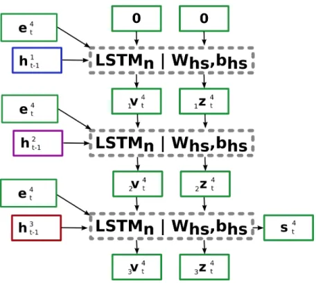
sample scenario is shown in Figure 3.1. The example objective that will be considered is the task of predicting the next position of the green agent (whose agent id is 4).
The overall sequence of operations for predicting the location of the green agent is shown in Figure 3.2. Each green box is a vector or tensor that is calculated for the green agent. Each box with a dashed gray border is an operation on vectors or matrices. The s4
t vector is the representation of the influence of neighboring agents
on the fourth agent (green agent) at timestep t. The e4
t vector is the representation
of the current coordinates of the fourth agent at timestep t. The coordinate and neighbor representations are used as inputs to the Agent-LSTM (LST Ma) along with
the previous hidden state (h4
t−1) and cell state (c4t−1), where the hidden and cell
states are specific to the green agent. The previous states will represent the previous trajectory of the green agent. The Agent-LSTM then outputs the next hidden and cell states along with an output vector. A fully-connected layer is applied to the output vector to output parameters of a Bivariate Gaussian that specifies the likely position of the green agent in the next timestep. The fully-connected layer is represented by Φ with weight matrix W and bias vector b . There is no activation function
Figure 3.2: Core Social-LSTM Architecture
applied in the Φ operation. The details of how the output parameters are used to define a probability distribution are discussed in Chapter 4 Design. For Social-LSTM, the probability distribution is specified by just 5 parameters. Equation ?? is the mathematical equivalent of Figure 3.2 for predicting the position of agent i at timestep t. oit, hit, cit =LST Ma(sit, e i t;h i t−1, c i t−1;Wa, ba) Θ4t = Φ(oit;WΘ, bΘ) (3.1)
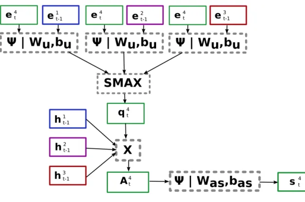
Figure 3.3 and Equation ?? show how the coordinate (eit) and neighbor (sit) em-bedding vectors are computed. The coordinate vector eit is just a fully connected embedding of the raw coordinate values with the weight matrix We and bias vector
be. Ψ denotes the embedding using a relu activation. A relu activation is a function
that is 0 when the input value is less than 0 and is equal to the input value when the input is greater than 0. The construction of the neighbor vector sit is much more involved. First, a tensor Pti is created as a grid with dimensions (k, k, l) where k is the number of cells in the width and height and l is the size of the hidden state from the Agent-LSTM. The indicator function 1mn is 1 when the input values are within
the mth row and nth column of the grid. The inputs to the indicator function are
the differences between each neighboring agent’s coordinates and the current agent’s coordinates. The value of every grid cell is the sum of the latent representations of all
Figure 3.3: Neighbor and Coordinate Representations for Social-LSTM
neighbors that exist in that cell (when the indicator function is 1). The grid is then embedded into a tensor by applying a fully-connected layer Ψ with weight matrixWps
and bias vector bps.
Figure 3.3 does not incorporate the hidden state of the blue agent in the grid because the blue agent’s current position is outside of the grid.
eit = Ψ(xit, yti;We, be) Pti(m, n,:) = X j∈Ni 1mn[x j t −x i t, y j t −y i t]h j t−1 sit = Ψ(Pti;Wps, bps) (3.2)
Like most neural networks, there are a number of hyper-parameters that must be set in order to fully specify the model. For Social-LSTM, the important hyper-parameters are the size of the grid (how much of the environment is included) and the granularity of the grid (number of cells). Selecting a grid size that is too small will mean that relevant neighbors that would affect the movement of the agent will not be considered. On the other hand, a large grid size may sacrifice the precision of the spatial position of each neighbor since the grid cells will each cover a large portion
large grid size (cover much of the environment) and a large number of cells to achieve high coverage and high spatial granularity, but there are several disadvantages to this. First, the matrixP and the weight matrixWpd will become enormous and will occupy
considerable memory during training and inference. Additionally, the network will have to learn more parameters, which generally requires more training data in order to encounter many training samples that include the agents in all of the cells.
3.1.5.2 Soft + Hardwired Attention
Fernando et al.[12] designed a novel sequence-to-sequence neural network architecture based on Social-LSTM. They postulate that a weakness of Social-LSTM is that the next position of the current agent is predicted using only a function of the hidden representation of the current agent and the social tensor of the hidden states of the neighbors at the current timestep. In their research, Fernando et al. use an attention mechanism to incorporate all previous hidden states of both the current agent and the neighboring agents when making predictions. This has the benefit of allowing the neural network to model how the agent reacts to different scenarios and including that information in subsequent predictions. The attention mechanism uses learned parameters to weight the previous states of the current agent and hardwired weights based on Euclidean distance to weight the neighbors’ previous hidden states. Additionally, the neural network is trained as a sequence-to-sequence model, so the model never represents the next position with a probability distribution like Social-LSTM. Rather, the first part of the network encodes a sequence of 20 time steps, which is then fed into the second part of the network that decodes the next 20 time steps.
Fernando et al. evaluated their architecture against Social-LSTM on the crowded Grand Central Station Dataset[58] and Edinburgh Informatics Forum Dataset[34].
Prior to fitting their model, Fernando et al. first clustered the trajectories based on destination and then trained separate models for each cluster. Their attention-based model was superior to Social-LSTM in each evaluation category and dataset. Since their architecture involves several departures from Social-LSTM, it is not obvious whether the attention mechanism in particular was the most important modification. Even the reduced model that omits information about neighbors performs nearly as well as Social-LSTM.
3.2 Deep Representations
Relatively straightforward convolutional neural networks and recurrent neural net-works have produced significant results in a variety of domains. However, deeper and more powerful neural network architectures have begun to show increased potential in recent years. This thesis relies on these modern designs; this section summarizes the relevant advances in neural network construction.
3.2.1 Attention in Neural Networks
Attention is the general concept of focusing on specific details. Humans have a well-developed capacity for attention. When someone is speaking, humans generally con-centrate on the speaker rather than the plain wall behind the speaker. When driving, humans focus on the road in front of them and nearby cars rather than the color of the sky. Of course, humans can also attend to things that are not relevant. Sometimes, human drivers look closely at accidents, causing them to subconsciously slow down. During uninteresting speeches, humans may decide to focus on the people they are sitting next to or the chores that need to be completed later.
over-In a similar way, it can be beneficial to endow neural networks with the ability to attend to certain aspects of the input rather than others. The key components of attention mechanisms in neural networks are the selection and representation of the information to attend to. Many attention mechanisms have been proposed, but the key distinctions for this thesis are hard versus soft attention and spatial versus tem-poral attention.
3.2.1.1 Soft and Hard Attention
Attention mechanisms have the potential to improve the accuracy and speed of neural networks since expensive processing can be applied only to the relevant parts of the inputs, and extraneous noise in the inputs can be ignored. However, training these powerful networks can be challenging. The design of the attention mechanism deter-mines how the model can be trained. If the attention mechanism is fully-differentiable (called “soft”) then the network can be trained using Backpropagation similar to most other neural networks. However, if the attention mechanism is not differen-tiable (called “hard”), then it is no longer possible to use simple Backpropagation. Therefore for “hard” attention mechanisms, Reinforcement Learning techniques are usually the method of choice for training.
An example of a “soft” attention mechanism is a weighted combination of all inputs. One part of the neural network will output a weight for each input, and the inputs times their weights is then fed into another part of the neural network for further processing. An example of a “hard” attention mechanism is the selection of a strict subset of the input. By only choosing some of the input to use, it is no longer possible to compute the gradients of the attention mechanism.
3.2.1.2 Spatial and Temporal Attention
A neural network can use attention mechanisms for attending on any type of data; however, there are two typical applications of attention - spatial and temporal. Some of the first attention mechanisms were applied in recurrent neural networks to attend to the state of the network at previous time steps. One of the best examples of this temporal attention is the seminal paper by Bahdanau et al. about Neural Machine Translation [4]. They used LSTMs to encode a sentence in one language and then more LSTMs to decode the sentence in a different language. The decoding LSTMs received input from the output of the encoding LSTM (as usual) but also from a weighted summation of the states of the encoding LSTM cells. The weights were computed using an alignment network (a type of attention). Even earlier, Graves used a similar methodology for handwriting generation[18]. Graves constructed a network that could attend to a windows of the input while generating handwritten characters.
Recently, researchers have considered spatial attention where a neural network is trained to attend to certain regions in a spatial domain (most often the attention focuses on a part of an image). An excellent example of spatial attention is the famous DRAW neural network created by Gregor et al. [19]. The DRAW model is a Variational Autoencoder that uses a recurrent neural network to read sections of an input image and then another set of recurrent neurons to reconstruct the input image by selecting regions of the output canvas and drawing to them. The DRAW network outputs images much like humans - by copying individual parts of the images at each timestep. The regions that DRAW attends to are based on the hidden state of the recurrent neural network from the previous timestep.