Pricing derivatives with stochastic volatility

(1)

n

Chen, Jilong (2016) Pricing derivatives with stochastic volatility.

PhD thesis.

http://theses.gla.ac.uk/7703/

Copyright and moral rights for this thesis are retained by the author

A copy can be downloaded for personal non-commercial research or

study, without prior permission or charge

This thesis cannot be reproduced or quoted extensively from without first

obtaining permission in writing from the Author

The content must not be changed in any way or sold commercially in any

format or medium without the formal permission of the Author

When referring to this work, full bibliographic details including the

author, title, awarding institution and date of the thesis must be given

Glasgow Theses Service

http://theses.gla.ac.uk/

(2)

Pricing Derivatives with Stochastic

Volatility

by

Jilong Chen

Submitted in fulfilment of the requirements for

the degree of Doctor of Philosophy

Adam Smith Business School

College of Social Sciences

University of Glasgow

(3)

Abstract

This Ph.D. thesis contains 4 essays in mathematical finance with a focus on pricing Asian option (Chapter 4), pricing futures and futures option (Chapter 5 and Chapter 6) and time dependent volatility in futures option (Chapter 7).

In Chapter 4, the applicability of the Albrecher et al.(2005)’s comonotonicity approach was investigated in the context of various benchmark models for equities and com-modities. Instead of classical L´evy models as in Albrecher et al.(2005), the focus is the Heston stochastic volatility model, the constant elasticity of variance (CEV) model and the Schwartz (1997) two-factor model. It is shown that the method delivers rather tight upper bounds for the prices of Asian Options in these models and as a by-product delivers super-hedging strategies which can be easily implemented.

In Chapter 5, two types of three-factor models were studied to give the value of com-modities futures contracts, which allow volatility to be stochastic. Both these two models have closed-form solutions for futures contracts price. However, it is shown that Model 2 is better than Model 1 theoretically and also performs very well empiri-cally. Moreover, Model 2 can easily be implemented in practice. In comparison to the Schwartz (1997) two-factor model, it is shown that Model 2 has its unique advantages; hence, it is also a good choice to price the value of commodity futures contracts. Fur-thermore, if these two models are used at the same time, a more accurate price for commodity futures contracts can be obtained in most situations.

In Chapter 6, the applicability of the asymptotic approach developed in Fouque et al.(2000b) was investigated for pricing commodity futures options in a Schwartz (1997) multi-factor model, featuring both stochastic convenience yield and stochastic volatility. It is shown that the zero-order term in the expansion coincides with the Schwartz (1997) two-factor term, with averaged volatility, and an explicit expression for the first-order correction term is provided. With empirical data from the natural gas futures market, it is also demonstrated that a significantly better calibration can be achieved by using the correction term as compared to the standard Schwartz (1997) two-factor expression, at virtually no extra effort.

In Chapter 7, a new pricing formula is derived for futures options in the Schwartz (1997) two-factor model with time dependent spot volatility. The pricing formula can also be used to find the result of the time dependent spot volatility with futures options prices in the market. Furthermore, the limitations of the method that is used to find the time dependent spot volatility will be explained, and it is also shown how to make sure of its accuracy.

(4)

List of Tables

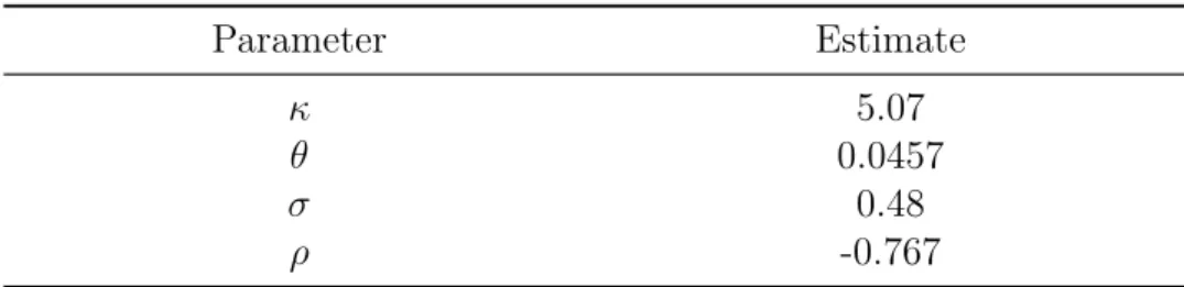
4.1 Parameters estimates for the Heston model . . . 40

4.2 Prices under the Black-Scholes model (monthly averaging) . . . 41

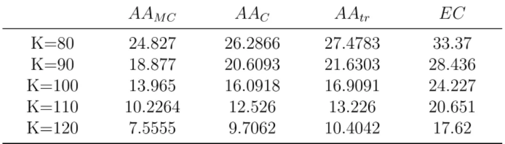
4.3 Prices under the Heston model (monthly averaging),θ= 0.0457. . . 43

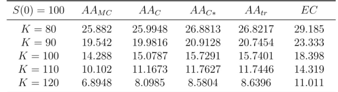
4.4 Prices under the Heston model (monthly averaging),θ= 0.5 . . . 43

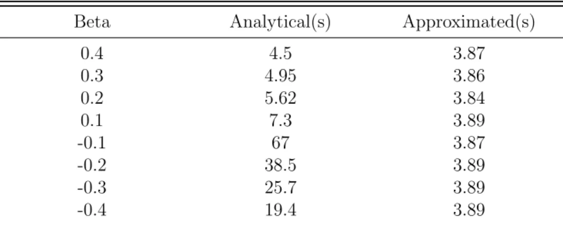
4.5 Computational time for determining the option price using the analytical non-central Chi-squared distribution and its approximated distribution . . . 44

4.6 Prices under the CEV model . . . 45

4.7 Prices under the Schwartz (1997) two-factor model (monthly averaging) . . . 46

4.8 Comparison under the Heston model . . . 49

4.9 Comparison under the Schwartz(1997) two-factor Model . . . 49

4.A.1 Strike prices for the hedge portfolio under the Black-Scholes model (monthly averaging) withS(0) = 100 andT = 1 . . . 51

4.A.2 Strike prices for the hedge portfolio under the Heston model (monthly averaging) with S(0) = 100,θ= 0.0457 . . . 52

4.A.3 Strike prices for the hedge portfolio under the Heston model (monthly averaging) with S(0) = 100,θ= 0.5 . . . 53

4.A.4 Strike prices for the hedge portfolio under the CEV model withS(0) = 100 . . . 55

4.A.5 Strike prices for the hedge portfolio under the Schwartz (1997) two-factor model (month-ly averaging) withS(0) = 100 . . . 56

4.A.6 Comparison under the CEV model . . . 58

5.1 Parameter estimates for three-factor model . . . 73

5.2 Parameter estimates for the Schwartz (1997) two-factor model . . . 73

6.1 Parameter choices for three-factor model . . . 96

6.2 Futures options prices . . . 97

6.3 Natural gas futures prices (GKJ4). . . 97

6.4 Natural gas futures call options prices . . . 98

6.5 Parameter estimation from market data for asymptotic two-factor model and standard two-factor model . . . 98

6.6 Natural gas futures call option prices from asymptotic two-factor solution . . . 99

6.7 Natural gas futures call option prices from the Schwartz (1997) two-factor model . . 99

6.8 The value of RSS for asymptotic two-factor model and standard two-factor model in terms of time maturity . . . 99

7.1 Natural gas futures prices . . . 112

7.2 European call natural gas futures options prices with different strike prices . . . 112

7.3 Estimated results of parameters . . . 113

(8)

7.5 Test result for first constraint . . . 116

(9)

List of Figures

2.1 The implied volatility of Amazon call options1 _{. . . .} ₁₄

5.1 The prices of futures contract . . . 65

5.2 Price comparison between three models . . . 68

5.3 The process of filter technology . . . 69

5.4 Model 2 forward curve, 50th . . . 75

5.5 Schwartz (1997) two-factor model forward curve, 50th. . . 75

5.7 Schwartz (1997) two-factor model forward curve, 100th . . . 75

5.9 Schwartz (1997) two-factor model forward curve, 200th . . . 76

5.B.1 Estimated spot price from Model 2 . . . 80

5.B.2 Estimated convenience yield from Model 2 . . . 80

5.B.3 Estimated volatility of the gold from Model 2. . . 80

5.B.4 Estimated spot price from the Schwartz (1997) two-factor model. . . 80

5.B.5 Estimated convenience yield from the Schwartz (1997) two-factor model . . . 80

5.B.6 Effectiveness of Model 2, Feb . . . 81

5.B.7 Effectiveness of Model 2, Apr . . . 81

5.B.8 Effectiveness of Model 2, Jun . . . 81

5.B.9 Effectiveness of Model 2, Aug . . . 81

5.B.10 Effectiveness of Model 2, Oct . . . 81

5.B.11 Effectiveness of Model 2, Dec . . . 81

5.B.12 Effectiveness of the Schwartz (1997) two-factor model, Feb . . . 82

5.B.13 Effectiveness of the Schwartz (1997) two-factor model, Apr . . . 82

5.B.14 Effectiveness of the Schwartz (1997) two-factor model, Jun . . . 82

5.B.15 Effectiveness of the Schwartz (1997) two-factor model, Aug . . . 82

5.B.16 Effectiveness of the Schwartz (1997) two-factor model, Oct . . . 82

5.B.17 Effectiveness of the Schwartz (1997) two-factor model, Dec . . . 82

5.B.18 Prices of futures contracts from Model 2 . . . 83

5.B.19 Prices of futures contracts from the Schwartz (1997) two-factor model . . . 83

5.B.20 Real futures contracts prices. . . 83

(10)

Acknowledgements

First of all, I would like to express my deepest gratitude to my principal supervisor Professor Christian-Oliver Ewald for his invaluable wisdom and insight that deepen and enrich my knowledge of mathematical finance, and his innumerable help and patience on every aspect of my research in the past 3-4 years.

I would also like to take this opportunity to thanks to Dr Yuping Huang, who en-couraged me at the beginning of my Ph.D. study and Zhe Zong, who gave me help in studying Kalman filter technique. I wish to thank all the follow friends, Huichou Huang, Yang Zhao, Xiao Zhang, Xuan Zhang and Suo Cao who give me chances to experience many interesting things beyond mathematical finance. I trust that all other people whom I have not specifically mentioned here are aware of my deep appreciation. Finally, I am deeply obliged to my parents and my wife for giving me the opportunity, support and freedom to pursue my interests — any success I have achieved as a Ph.D. student is instantly related to them.

(11)

Dedication

To my parents, Dongyao Chen and Zhaomei Cai and my wife, Liying Zhang.

(12)

Declaration

I declare that, the materials of this Ph.D. thesis is the result of my own work except where explicit reference is made to the contribution of others. These materials may also appear as published and/or working papers co-authored with my principal super-visor Professor Christian-Oliver Ewald (Chapter 4, Chapter 6 and Chapter 7), and my colleague Zhe Zong (Chapter 5). The bulk of materials (mathematical derivations and discussions) in Chapter 4, Chapter 6 and Chapter 7 are the results of my own ideas. Except the introduction of the Kalman filter technique and figures from the Kalman filter technique, the rest of Chapter 5 are undertaken by myself. Furthermore, part of materials from Chapter 6 are presented at 2015 Quantitative Methods in Finance conference.

Published papers resulting from this thesis.

[1] Chen, J. and Ewald, C.O., On the Performance of the Comonotonicity Approach for Pricing Asian Options in some Benchmark Models from Equities and Commodities, (to appear in) Review of Pacific Basin Financial Markets and Policies.

Jilong Chen July 2016

(13)

Chapter 1 Introduction

Options have been important financial instruments for hedging, speculation, arbi-trage, and risk mitigation purposes in the financial markets over the past few years. They are fundamentally different from forward and futures contracts. For options’ holders, they have the right to do something, but the holder does not have to exer-cise this right. However, in a forward or futures contract, the two parties have to do certain actions when the contract is expired. Furthermore, it costs nothing to enter into a forward or futures contracts, whereas a premium is necessary to buy an option contract.

Generally, there are two types of options. A call option gives the buyer (the owner or holder of the option) the right, but not the obligation, to buy an underlying asset or instrument at a specified price on a specified date. A put option gives the buyer (the owner or holder of the options) the right, but not the obligation, to sell an underlying asset or instrument at a specified price on a specified date. The price in the contract is known as the strike price; the date in the contract is known as the expiration date.

For a call option, it will normally be exercised when the strike price is below the market value of the underlying asset. The cost to have the underlying asset to the buyer is the strike price plus the premium. Compared with those who do not hold call option, the profit to the call option holder is the difference between the market price and strike price minus the premium. When the strike price is above the market value of the underlying asset, a call option will normally not be exercised. The loss to a call option holder is the premium, compared with those who do not hold call option.

For a put option, it will normally be exercised when the strike price is above the market value of the underlying asset. Compared with the non-put option holder, a put option holder can benefit from the profit of the difference between the market price and strike price minus the premium. When the strike price is below the market value of the underlying asset, a put option normally will not be exercised. The loss to a put option holder is the premium, compared with a non-put option holder.

Whether the call option or put option, the income to the option seller is the pre-mium, and the loss to the option seller is the potential increment or decrement of the underlying price in the future market, depending on the form of option.

In terms of the underlying asset or the calculation of how or when the investor receives a certain payoff, options can be defined as vanilla options and exotic options.

(14)

Vanilla options contain European style options and American style options; the main difference being that American style options can be exercised before the expiration date, whereas the European style options can only be exercised on the expiration date. Therefore, generally American style options will be more expensive than European style options. They are often traded on exchange markets, and most options traded on exchange markets are American style. However, compared with American style options, in general, European style options are easier to analyse and frequently used as a benchmark for American style options.

An exotic option is an option that has more complex features than vanilla options. These features could reflect on the changing of the underlying, the payoff type, and the manner of settlement. For example, the payoff for a look-back option at maturity is not just on the value of the underlying instrument at maturity, but its maximum or minimum value during the option’s life. Therefore, exotic options are generally traded on the over-the-counter (OTC) markets.

1.1 Asian Option

An Asian option is one of exotic options, in which the underlying is the average of a financial variable, such as prices of equities, commodities, interests or exchange rates. The pricing of such derivatives has been of utmost interest ever since trading started in the mid 1980’s, initially mostly on OTC markets but for the last few years also on exchanges such as the London Metal Exchange. The most common claim of fixed strike asian call option is:

C(T) =max(A(0, T)−K,0)

where Adenotes the average price for the period [0, T], andK is the strike price. The equivalent put option is given by:

P(T) =max(K−A(0, T),0)

The average used in the calculation of Asian options can be defined in an arithmetic average or a geometric average. For example, in the case of discrete time, an arithmetic Asian option is:

A(0, T) = 1 N N X i Sti

and a geometric Asian option is:

A(0, T) = N v u u t N Y i Sti

An Asian option has many obvious advantages. Firstly, because of the average feature, arithmetic Asian options can reduce the market risk of underlying assets over a

(15)

certain time interval. Furthermore, arithmetic Asian options are typically less expensive than European or American options. In addition, they are also more appropriate than European or American options for meeting certain needs of the investors. Taking an investor who holds a large number of foreign currency exchanges as an example, the investor does not want to face the risk of currency exchanges, because the exchange rate may change everyday and will be highly volatile in the future. In this situation, an Asian put option can help the investor to reduce the exposure to the uncertain exchange rate, thereby guaranteeing that the average exchange rate is realized above a certain level during that time.

If Sti is assumed to follow a log normal distribution, a closed-form solution for the

value of a geometric Asian option can be found because geometric average of log normal random variable is still log normal. These closed-form expressions are very similar to formulas for pricing vanilla options in the Black-Scholes model.

However, even in the Black-Scholes world, there is no simple closed-form solution for the value of arithmetic Asian options, since the arithmetic average of log normal random variables is no longer log normal. It is very difficult to price arithmetic Asian options since their payoff is determined by the value of arithmetic average of some underlying asset during a pre-set period of time. Generally, people can use the Monte Carlo simulation technique and partial differential equation method to get its price. Nevertheless, for the purpose of getting an accurate price for an arithmetic Asian op-tion, the Monte Carlo simulation technique often requires a large amount of simulation trials. For example, one may use at least 100,000 simulation trials for giving the val-ue of an arithmetic Asian option. Therefore, in general, the Monte Carlo simulation technique is very time-consuming in terms of getting an accurate result.

Geman and Yor(1993,1996) derived analytic representations in the form of complex integrals for the price of a normalized Asian call option in the Black-Scholes model. This fundamental work was followed up and extended upon by a large number of authors, uncovering important relations to fundamental problems in probability theory and classical functions. The demands of financial practitioners however have long moved beyond the Black-Scholes model and the model error imposed by the Black-Scholes assumptions often outweighs any computational progress that some analytic formulas and techniques based on the Black-Scholes assumptions seem to offer.

1.2 Commodities Futures Option

Futures option, also known as option on futures, is similar to stock option, but the underlying is a single futures contract. It was first traded on an experimental basis in 1982 which was authorized by the Commodity Futures Trading Commission in the US. In 1987, permanent trading was approved and since then the popularity of futures options has grown very quickly with investors. Generally, they are American style options and traded on exchange markets. However, for some energy commodities, like crude oil and natural gas, the futures options are both European style and American style and are traded on exchange markets as well.

The buyer of a futures option has the right, but not the obligation, to enter into a futures contract at a certain futures contract price by a certain date. The price in the

(16)

contract is known as the strike price; the date in the contract is known as the expiration date. Generally, the expiration date of futures options will be one day or two days in advance, compared with the expiration date of corresponding futures contracts.

A call futures option gives the holder the right to enter into a long futures contract at the strike price when the strike price of the futures option is lower than the price of a futures contract in the market. In this case, the holder will benefit from a cash amount, which equals the difference between the settlement futures contract price and the strike price. However, the holder must pay a premium to buy this right; thus, if the futures option is not exercised, the premium will be the capital loss to the holder. A put futures option gives the holder the right to enter into a long futures contract at the strike price when the strike price of the futures option is higher than the price of a futures contract in the market. In this case, the holder will benefit from a cash amount, which equals the strike price minus the most recent settlement futures contract price. However, like the call futures option, a premium must be paid to have the long position in the futures option. If the strike price of the futures option is lower than the price of the futures contract in the market, the futures option will generally not be exercised; thus, the holder of the futures option will lose the premium.

The seller must be in the opposite futures position when the buyer exercises their right; however, no matter how the futures market changes in the future, the profit to a seller is the premium, which is paid by the buyer.

It is important to note that the underlying of a futures option is the futures contract, not the commodity, since an option on a commodity and an option on a futures contract is different. For example, a call option on crude oil will give the holder the right to buy crude oil at a price that equals the strike price; however, the holder of a call option on crude oil futures has the right to benefit from the difference between the futures contract price and strike price. If the crude oil futures option is exercised, the holder will also receive the corresponding futures contract. Therefore, the futures option price is related to the futures contract price, not the commodity price, even though the futures contract price tracks the corresponding commodity price closely. However, when the expiration date of a futures contract is the same as the expiration date of an option on a commodity, that is, the futures contract price equals the commodity price, then these two options are equivalent.

The popularity of trading options on futures contracts rather than options on the commodities is because of three main reasons. Firstly, a futures contract is more liquid than the commodity and the price of a futures contract can be known immediately from trading on the futures exchange. However, the commodity price can be known only by contacting one or more dealers. Secondly, a futures contract is easier to trade than a commodity. For instance, it is much easier to deliver a crude oil future contract than to deliver crude oil itself. Thirdly, in general, the delivery of a commodity will not happen since a futures contract will often be closed before the delivery date. Therefore, a futures option is normally settled in cash in the end, which is appealing to many investors who are interested in margin and leverage.

The futures option actually belongs to the vanilla option, thus if the futures contract price is assumed to follow a log normal process, a closed-form solution for the value of futures option can be obtained. The pricing formulas for European futures option

(17)

were first presented by Fischer Black in 1976. The Black model is similar to the Black-Scholes model except that the underlying is the futures contract and the volatility is the futures contract volatility. Following Black’s work, the pricing futures option has been further studied by many authors and some assumptions of the Black model have been eased. However, similar to the Black-Scholes world, some errors imposed by assumptions (e.g., constant volatility) were not solved by these extended models.

1.3 Structure of Thesis

It is natural to view volatility as a stochastic variable because it is clearly not constant. In this thesis, highly efficient methods to price derivatives with stochastic volatility are developed. Specifically, a tight upper bounds for the prices of Asian options in the Heston stochastic volatility model, the constant elasticity of variance (CEV) model and the Schwartz (1997) two-factor model are presented. In terms of stochastic spot volatility, also shown are closed-form solutions for the futures contract price and a very accurate approximated result for the futures option in the Schwartz (1997) two-factor model with stochastic spot volatility. Lastly, the behaviour of time dependent volatility in the Schwartz (1997) two-factor model is investigated.

In Chapter 2, firstly presented are some basic mathematical theorems that are re-lated to this thesis, including fundamental theorem of asset pricing, stochastic calculus, Itˆo’s lemma and cholesky decomposition. After that, the Black-Scholes model and the stochastic volatility model for financial derivatives are introduced.

In Chapter 3, there will be a review of the literature of pricing Asian option, pricing futures contract and pricing futures option, which is not very long since a brief literature review is given for the corresponding topics in each chapter.

In Chapter 4, there will be a brief overview on the theoretical background of the

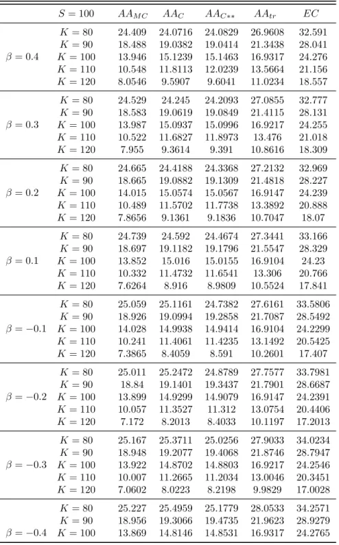
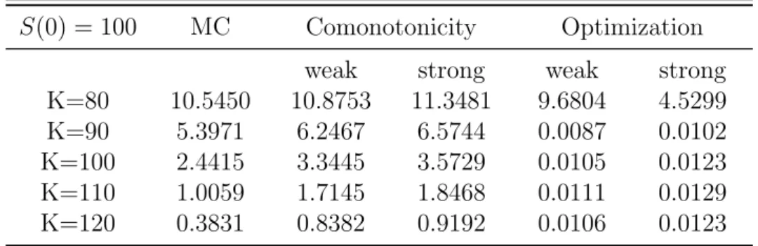
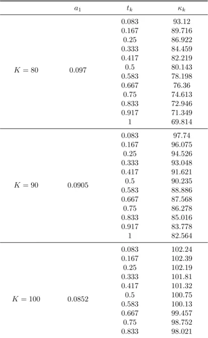
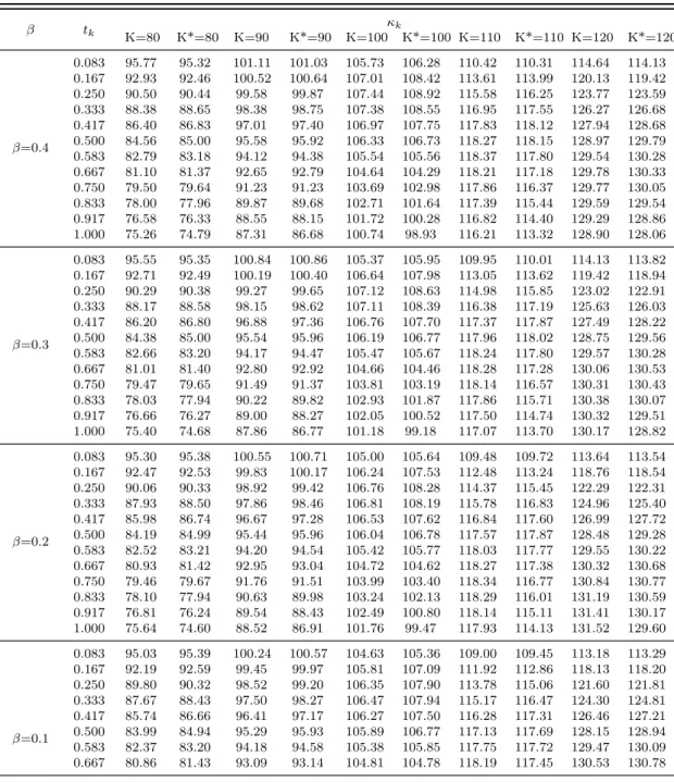
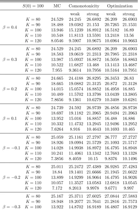
Albrecher et al. (2005)’s approach to obtain the upper bound for an arithmetic Asian option and its corresponding static super-hedging strategy in form of European call options. Then, the application of Albrecher et al. (2005)’s approach in the Heston model, the CEV model and the Schwartz (1997) two-factor model is examined. After that, the performance of each model is compared and numerical illustrations for the corresponding hedging strategies are provided. This analysis includes Monte Carlo prices, the comonotonic-upper-bound prices for an arithmetic Asian call option and two further static super-hedging prices, including the trivial static super-hedging price using a single European call option only (with the same strike price and maturity) as well as a static super-hedging price where all call options in the portfolio share the same strike. Section 5 provides a comparison between the comonotonicity approach and an alternative optimization based method. Finally, there is a summary of the main conclusions of this chapter.

In Chapter 5, based on the Schwartz (1997) two-factor model, two types of three-factor models are developed, to give the value of a commodity futures contract, which allow volatility to be stochastic. It is shown that closed-form solutions for futures contracts price can be derived within these two models. After that, the Kalman filter technology and an extended Kalman filter algorithm are discussed to estimate the

(18)

parameters in these two new developed models. Then, an empirical test with gold data for one of new developed models will be provided, and also its comparison to the results of the Schwartz (1997) two-factor model. Finally, there is a summary of the main conclusions of this chapter.

In Chapter 6, firstly, the theoretical background of the asymptotic approach is introduced and it is shown how to use this method to find the expression for the price of a futures option in the Schwartz (1997) two-factor model with stochastic spot volatility. After that, it is shown that the asymptotic formula has a better performance than the Schwartz (1997) two-factor model both in simulated data and real market data. Finally, there is a summary of the main conclusions of this chapter.

In Chapter 7, closed-form expressions for European style futures options with time dependent spot volatility are derived firstly. Secondly, it is shown how to use these expressions to find time dependent spot volatility for futures options with market data. After that, it is also shown how to examine the time dependent spot volatility is correct or not. Finally, there is a summary of the main conclusions of this chapter.

(19)

References

Albrecher, H., J. Dhaene, M. Goovaerts, and W. Schoutens, 2005, Static hedging of asian options under levy models, The Journal of Derivatives 12, 63–73.

Geman, H´elyette, and Marc Yor, 1993, Bessel processes, asian options, and perpetuities,

Mathematical Finance 3, 349–375.

Geman, H´elyette, and Marc Yor, 1996, Pricing and hedging double-barrier options: A probabilistic approach, Mathematical finance 6, 365–378.

(20)

Chapter 2 Mathematical Background

2.1 Mathematical Theorem

One of the key problems in pricing derivatives is how to derive the fair value of derivatives (e.g., futures, options etc). The fair price will not give investors the opportunity to obtain extra profit without any risks. Hence, a no arbitrage world is very important, some basic background of arbitrage-free world will be introduced firstly.

2.1.1 Fundamental Theorem of Asset Pricing

In a multi-period market, investors can gather information over time; hence, it is needed to take care about the evolution over time of the information available to investors. This leads to the probabilistic concepts of a σ-algebra, a filtration and a probability measure.

Definition 2.1. A collection F of subsets of the state space Ωis called a σ-algebra (or

σ-field) whenever the following conditions hold:

• Ω∈ F,

• If F ∈ F, then Fc= Ω\F ∈ F,

• If Fi ∈ F for i∈N then S∞i=1Fi ∈ F.

A state space Ω can be seemed as events or samples space, for example, the infor-mation that stock price changes over a year. σ-algebra is supposed to model a certain quantity of information, the larger the σ-algebra, the information conveyed by the σ -algebra is richer. In the example above, F could be the information that stock price goes up or goes down one day, one week or one month. In reality, a stock may in a state of suspension which is included in the state space Ω, however, this is not included in F.

Definition 2.2. A sequence (Ft)0≤t≤T ofσ-algebra onΩis called a filtration ifFs ⊂ Ft

(21)

The main idea behind a filtration is to find a sequence F which records the infor-mation dynamically, that is, the inforinfor-mation in F will be increased in time. If _F is a filtration, then a stochastic process (Xt) (e.g., stock price) is called F-adapted.

Lastly, the definition of probability measure is similar to that of σ-algebra, except that the probability is constrained between 0 and 1. Without probability measure, for example, investors can only say the stock price is very likely to rise, however, with probability measure, ’very likely’ can be measured numerically.

Now the problem becomes which probability measure should be used for pricing since different investors have different attitudes on risk. This leads us into the world of risk-neutral probability measure.

Definition 2.3. A measure _Q on Ω is called a risk-neutral probability measure for a general multi period market model if

• Q(w)>0 for all w∈Ω, • EQ( 1 1+rS i t+1 | Ft) = Sti for all 0≤t≤T −1

In terms of mathematical finance, risk-neutral probability measure is a result of measure change, which is a mathematical tool for convenient calculation. In risk-neutral world, the present value of a derivatives claim is its discounted expected value by risk-free rate (r), which is the key for pricing derivatives by Monte Carlo method. The second condition also leads us to martingale.

Definition 2.4. A (Ft)-adapted process (St) on a finite probability space (Ω,F,P) is

called a martingale if and only if for all s < t

EP(St| Fs) =Ss

Because the discounted stock price ( ˆSi

t) for i = 1, ..., n are martingales under risk measure _Q, risk measure _Q are often referred to as martingale measures. In terms of finance, martingale has two meanings. Firstly, with current information, investors can only know the current stock price at most, that is, the stock price cannot be predicted with current information. Secondly, if market is completed or efficient, all information can be obtained before current time. It is also an implication of the efficient market hypothesis.

When it comes to completed market, it comes with no arbitrage opportunity. There-fore, martingale measure can be a useful criterion to check whether an arbitrage op-portunity exists or not. The next two theorems are fundamental to the modern theory of mathematical finance. In general sense, they reveal the relationship between risk-neutral measure and no arbitrage opportunity. (see, e.g., Harrison and Kreps (1979),

Harrison and Pliska (1981) andDelbaen and Schachermayer (1994))

Theorem 1 (The First Fundamental Theorem of Asset Pricing). If there is a risk-neutral measure, then there are no arbitrage opportunity in market.

(22)

The first theorem is important because it ensures a fundamental property of market models. Although it is not realistic, it is often assumed that the market is complete for market model (for instance the Black-Scholes model). With this assumption, all contingent claim in the market can be replicated. The next theorem implicates that there is only one replication strategy for derivatives securities. The replication strategy is typically achieved by assembling a portfolio which value is equal to the the value of derivatives.

Theorem 2 (The Second Fundamental Theorem of Asset Pricing). If there is no arbitrage strategies in market, then there exist a risk-neutral measure.

2.1.2 Stochastic Calculus

Now two important tools in mathematical finance for pricing derivatives will be introduced in this section.

A stochastic process St is called Itˆo process if

dSt=µtdt+σtdWt (2.1) whereµtis called drift,σtis the volatility or diffusion parameter,dWtis the infinitesimal increment of Brownian motion.

This above equation is also referred to stochastic differential equation (SDE). To study the SDE world, the following rules of computation is fundamental, so called stochastic calculus. dWt·dWt=dt also, dWt·dt = 0 dt·dWt = 0 dt·dt = 0

Itˆo process is an important tool for pricing derivatives, and Itˆo lemma play a key role in it.

Theorem 3 (Itoˆ Lemma). If stochastic process St is a Itoˆ process and F(S, t) is

a 2-times continuously differential function on S and t, then F(S, t) has a stochastic process given by dF = (Ft+µtFS+ 1 2σ 2 tFSS)dt+σtFSdWt

Itˆo Lemma is the chain rule of stochastic calculus and it can also be applied into multi-variate stochastic processes,

dF = (Ft+ n X i=1 µiFi+ 1 2 n X i=1 n X j=1 σjσjρijFij)dt+ n X i=1 σiFidWi(t) (2.2)

(23)

where Fi = _∂S∂F_i, Fij = ∂

2_F

∂SiSj and ρijdt=dWidWj.

2.1.3 Cholesky Decomposition

It is hard to find a closed-form solution for derivatives with multi-variate stochastic process; in practice, it is often given the value of derivatives by the Monte Carlo method and Cholesky decomposition is commonly used in this method for simulating systems with multiple correlated variables. In mathematic term, the Cholesky decomposition or Cholesky factorization is a decomposition of a Hermitian, positive-definite matrix (A) into the product of a lower triangular matrix (L) which is real and positive diagonal entries and its conjugate transpose (LT_{), that is} _A₌_L_·_LT_.

There are various methods for calculating the Cholesky decomposition, one of them is the Cholesky-Banachiewicz and Cholesky-Crout algorithms.

If the equation is written as:

A =L·LT =      L11 0 . . . 0 L21 L22 . . . 0 .. . ... . .. ... Li1 Li2 . . . Lii           L11 L21 . . . Li1 0 L22 . . . Li2 .. . ... . .. ... 0 0 . . . Lii      (2.3) where Li,i = v u u tA_i,i− i−1 X k=1 L2 i,k (2.4) and Li,j = 1 Lj,j Ai,j− j−1 X k=1 Li,kLj,k ! (2.5) for i > j.

For a simplified example, if two correlated Brownian motion x1 and x2 are needed

to generate for the use of the Monte Carlo method. One just needs to generate two uncorrelated Gaussian random variables z1 and z2 and set x1 = z1 and x2 = ρz1 +

p

1−ρ2_z 2.

2.2 Mathematical Models

The main question of pricing derivatives is how the value of derivatives depends on the underlying price and time, in mathematic term, that is, what is the exact expression for the value of derivatives. In 1973, Black, Scholes and Merton answered this question in their work on pricing options, that is, the Black-Scholes model. This model is the queen in option pricing world and has a significant influence on mathematical finance,

(24)

changing the face of finance. It is also widely used in practice by people who works in derivatives, whether they are salesmen, traders or quants. However, there are some of flaws in the assumptions of the Black-Scholes model, which may lead the model’s price far away from its real market price. For example, exotic options are frequently even more sensitive to the level of volatility than standard European style option, thus the price given by the Black-Scholes model can be widely inaccurate. Therefore, people are motivated to find models to take volatility into account when pricing options. To this extent, stochastic volatility models are particularly successful since they can capture, and potentially explain the smiles, skews and other structures in terms of volatility which have been observed in options market. In this section, there will be an overview on the Black-Scholes model and stochastic volatility models.

2.2.1 Black-Scholes Model

Even though all of the assumptions can be shown to be wrong to a greater or lesser extent, the Black-Scholes model is very popular because it is very simple and can provide an easy, quick result for the value of options. Therefore, it is often treated as a benchmark model that other models can be compared. However, it should be noticed that the formation mechanism of option price is not changed by the Black-Scholes model, but is always decided by the market demand and supply. The most important part in the Black-Scholes model is that they provide ideas about delta hedging and no arbitrage. This section reviews the delta hedging and no arbitrage in the Black-Scholes model theoretically.

Firstly, the Black-Scholes model assumes that the stock price is satisfied with an Itˆo process:

dSt=Stµtdt+StσtdWt (2.6) where µis the return of the stock price and σ is the volatility of stock price.

Now buying an option V(S, t) and selling underlying S with some quantity ∆ to construct a portfolio Π at time t, that is:

Π =V(S, t)−∆S (2.7) The change of the value of this portfolio from time t to t+dt is:

dΠ =dV(S, t)−∆dS (2.8) Note that ∆ is constant during the time step.

From Itˆo lemma, one can have:

dV = ∂V ∂tdt+ ∂V ∂SdS+ 1 2σ 2_S2∂2V ∂S2dt (2.9)

Thus the portfolio becomes:

dΠ = ∂V ∂t dt+ ∂V ∂SdS+ 1 2σ 2_S2∂2V ∂S2dt−∆dS (2.10)

(25)

Now the right-hand side of the portfolio contains the deterministic term and random term, which are those with dt and dS respectively. The random term can be seemed as risk in the portfolio:

∂V ∂S −∆

dS (2.11)

To eliminate this risk, one could carefully choose a ∆: ∆ = ∂V

∂S (2.12)

In this way, the randomness is reduced to zero, this perfect elimination of risk is generally called delta hedging.

Choosing the quantity ∆ as suggested above, the portfolio changes by:

dΠ = ∂V ∂t dt+ 1 2σ 2_S2∂2V ∂S2dt (2.13)

Since the portfolio now is riskless, that means, there is no arbitrage opportunity, one can get:

dΠ =rΠdt (2.14)

Therefore, with some substitutions, dividing by dt and rearranging, one can ob-tained the Black-Scholes equation:

∂V ∂t + 1 2σ 2_S2∂ 2_V ∂S2 +rS ∂V ∂S −rV = 0 (2.15)

This equation was first written down in 1969, but the derivation of the equation was finally published in 1973. It is a linear parabolic partial differential equation. In fact, almost all partial differential equations in finance are of a similar form, meaning that if you have two solutions of the equation then the sum of these is itself also a solution.

Solving the Black-Scholes equation, one could get an analytical or closed-form so-lution for options price. In terms of European call option (C(S, t)):

C(S, t) =SN(d1)−Ke−r(T−t)N(d2) (2.16) where d1 = log(_KS) + (r+1₂σ2)(T −t) σ√T −t , d2 = d1−σ √ T −t.

and N(·) is the standard normal cumulative distribution function:

N(x) = √1 2π Z x −∞ e−t 2 2 dt (2.17)

(26)

With the Black-Scholes pricing formula, one could use the market value of the option to calculate the value of volatility for this option price. This volatility is called implied volatility. When the implied volatilities for market prices of options written on the same underlying price are plotted against a range of strikes and maturities, the resulting graph is typically like a smile, as shown in Figure2.1. This observation shows the constant volatility assumption is not true.

480 500 520 540 560 580 600 620 640 660 680 0.4 0.5 0.6 0.7 0.8 0.9 1

Strike Prices of Call Options

Implied Volatility

Implied Volatility of Call Options

Figure 2.1: The implied volatility of Amazon call options1

2.2.2 Stochastic Volatility Models

It has been seen that volatility does not behave how the Black-Scholes equation would like it to behave; it is not constant, it is not predictable, it is not even directly observable. There is a plenty of evidence that the log returns on equities, currencies and commodities are not normally distributed. Actually they have higher peaks and fatter tails than predicted by a normal distribution. Volatility has a key role to play in the determination of risk and in the valuation of derivatives. In this section, there will be a review of models for options valuation with stochastic volatility.

Now, the value of derivatives (V) depends on underlying priceS, timetand volatil-ity σ, that is, V =V(S, σ, t). One can assume the underlying price and volatility have following stochastic process:

dSt =Strdt+σStdW1

dσt=a(S, σ, t)dt+b(S, σ, t)dW2

(2.18) and two increment Brownian motions have a relationship, dW1·dW2 =ρdt.

It can be found that the choice of functions a(S, σ, t) andb(S, σ, t) is the key to the evolution of the volatility. Note that the volatility is not a tradable asset in market, hence it is not easy to hedge the risk or randomness from stochastic volatility. Be-cause there are two sources of randomness, the option must be hedged with two other contracts, one being the underlying asset as usual, but now it is also needed another option to hedge the volatility risk.

1_{The implied volatility is computed from Amazon equity options on Nasdaq with 3 weeks expiration}

time. Data are obtained from Yahoo Finance on April 28, 2016. The underlying price is 622.83 on that date

(27)

Considered a portfolio Π which contains one option with valueV(S, σ, t), a quantity

−∆ of the asset and a quantity−∆1 of another option with value denoted byV1(S, σ, t),

then one can have:

Π =V −∆S−∆1V1 (2.19)

The jump of the value of this portfolio in one infinitesimal time step dt is:

dΠ = ∂V ∂t + 1 2σ 2_S2∂2V ∂S2 +ρσSb ∂2_V ∂S∂σ + 1 2b 2∂2V ∂σ2 dt −∆1 ∂V1 ∂t + 1 2σ 2_S2∂ 2_V 1 ∂S2 +ρσSb ∂2V1 ∂S∂σ + 1 2b 2∂ 2_V 1 ∂σ2 dt + ∂V ∂S −∆1 ∂V1 ∂S −∆ dS+ ∂V ∂σ −∆1 ∂V1 ∂σ dσ. (2.20) where Itˆo lemma has been used on functions of S,σ and t.

Clearly one wish to eliminate all randomness by setting

∂V ∂S −∆1 ∂V1 ∂S −∆ = 0 (2.21) and ∂V ∂σ −∆1 ∂V1 ∂σ = 0 (2.22) so ∆1 = ∂V ∂σ/ ∂V1 ∂σ (2.23) and ∆ = ∂V ∂S −∆1 ∂V1 ∂S (2.24)

Again, by using no arbitrage argument that the return on a risk-free portfolio must be equal to the risk-free rate, this riskless portfolio becomes:

dΠ = ∂V ∂t + 1 2σ 2_S2∂2V ∂S2 +ρσSb ∂2_V ∂S∂σ + 1 2b 2∂2V ∂σ2 dt −∆1 ∂V1 ∂t + 1 2σ 2 S2∂ 2_V 1 ∂S2 +ρσSb ∂2V1 ∂S∂σ + 1 2b 2∂2V1 ∂σ2 dt = rΠdt=r(V −∆S−∆1V1)dt. (2.25)

This equation can be rearranged by collecting allV terms on the left hand side and allV1 terms on the right hand side, that is:

∂V ∂t + 1 2σ 2_S2∂2_V ∂S2 +ρσSb ∂2_V ∂S∂σ + 1 2b 2∂2_V ∂σ2 +rS ∂V ∂S −rV ∂V ∂σ = ∂V1 ∂t + 1 2σ 2_S2∂2_V 1 ∂S2 +ρσSb ∂2_V 1 ∂S∂σ + 1 2b 2∂2_V 1 ∂σ2 +rS ∂V1 ∂S −rV1 ∂V1 ∂σ (2.26)

(28)

Now the left hand side is a function of V only and the right hand side is a function of V1 only. Because the two options will typically have different payoffs, strikes or

time of expiration, the only way that this can be is for both sides to be equal to some functions, depending only on variable S, σ and t. Thus, it can be obtained at the general PDE for stochastic volatility:

∂V ∂t + 1 2σ 2_S2∂ 2_V ∂S2 +ρσSb ∂2V ∂S∂σ + 1 2b 2∂ 2_V ∂σ2 +rS ∂V ∂S −rV =−(a−λb) ∂V ∂σ (2.27)

Conventionally, the function λ(S, σ, t) is called the market price of volatility risk since it tells us how much of the expected return of V is explained by the risk of volatility in market.

It is hard to solve above mentioned PDE, generally one can use numerical method to find the result. However, there are some popular models which can find analytical solutions for European options with stochastic volatility.

Hull & White

Hull & White considered both general and specific volatility modeling. The most important result of their analysis is that when the stock and the volatility are uncor-related and the risk-neutral dynamics of the volatility are unaffected by the stock (i.e.

a−λb and b are independent of S ) then the fair value of an option is the average of the Black-Scholes values for the option, with the average taken over the distribution

σ2.

One of the risk-neutral stochastic volatility model considered by Hull & White is:

d(σ2) =c(d−σ2)dt+eσ2dW2

Heston

However, empirical study shows the correlation for the stock and the volatility is not zero. Heston (1993) gives the following model which can give a closed-form solution for European options when the stock and volatility are correlated.

dS = µSdt+√vSdW1

dv = λ(θ−v)dt+η√vdW2

ρdt = dW1dW2

Ornstein-Uhlenbeck (OU) process

In addition, the following model can match the data well, in the long run, volatility is log normally distributed in this model.

d(y) = (c−dy)dt+edW2

(29)

References

Delbaen, Freddy, and Walter Schachermayer, 1994, A general version of the fundamen-tal theorem of asset pricing, Mathematische annalen 300, 463–520.

Harrison, J Michael, and David M Kreps, 1979, Martingales and arbitrage in multi-period securities markets, Journal of Economic theory 20, 381–408.

Harrison, J Michael, and Stanley R Pliska, 1981, Martingales and stochastic integrals in the theory of continuous trading, Stochastic processes and their applications 11, 215–260.

(30)

Chapter 3 Literature Review

3.1 Pricing Asian Option

Accurate pricing for an arithmetic Asian option is really an important problem in practice. Different methods to this problem can be subdivided into three parts: the Monte Carlo method, the Partial Differential Equation (PDE) approach and the Bound Technique.

Boyle(1977) introduced Monte Carlo simulation for pricing option value to finance field. As he claimed, Monte Carlo simulation has many obvious advantages. Firstly, the Monte Carlo method is very flexible with distribution which describes the returns on the underlying stock. That means, in the Monte Carlo method, changing the under-lying distribution merely involves generating the random variates by different process. Secondly, the Monte Carlo method does not need the distribution which generates the return on the underlying stock with an analytical expression. This advantage makes pricing option value based on the empirical distribution of stock returns become possi-ble. Furthermore, the Monte Carlo method allows a distribution of stock return to solve any of the parameters of the problem rather than a point estimate. For instance, since the parameter is usually estimated from the empirical data, the Monte Carlo method can give a confidence interval to examine the accuracy of the estimators, which may be useful in some problem with regard to the variance.

Since then, with the popularity of computer, this approach is widely used by many authors. Kemna and Vorst (1990) pointed out that it is impossible to find an explicit formula for an arithmetic Asian option and explain it concretely. Also, they found the value of arithmetic Asian call option cannot readily be obtained by a finite difference method. Therefore, they applied the Monte Carlo method to price and hedge arithmetic Asian call options. As previously studied, the logarithm of stock price follows normal distribution with mean (r−1

2σ

2₎₍_T₋_t_{) and variance}_σ2p

(T −t)ε, thus the stock price can be expressed as:

ST =St·exp (r− 1 2σ 2₎₍_T ₋_t_{)) +}_σ2₍_T ₋_t₎ (3.1) whereST is the stock price at timeT,Stis the stock price at timet,randσare constant,

(31)

representing the expected rate of return and the volatility of stock price respectively, and ε is a random number that followed by standardized normal distribution N(0,1).

Assume: A(T) = 1 n+ 1 n X i=0 S(Ti) ! (3.2)

Then, the price of arithmetic Asian call option was calculated as:

C =e−r(T−t)max(A(T)−K,0) (3.3) where K is the strike price.

In general, as Boyle et al.(1997) described, the Monte Carlo method follows three steps. Firstly, according to the risk-neutral measure, simulate sample paths of the underlying state variables over the relevant time horizon. For example, use Equation (3.1) to simulate the stock price under risk-neutral probability at each node of exercise opportunity. Then, evaluate the discounted cash flow of an underlying asset on each sample path, according to the structure of the underlying asset in the question. For example, use Equation (3.2) and Equation (3.3) to calculate the value of arithmetic Asian call options. At last, average the discounted cash flow among all sample paths.

Broadie and Glasserman (1996) pointed out that Monte Carlo simulation is a valu-able approach for pricing options which do not have closed-form solutions and it is very suitable for pricing Asian options. However, Joy and Tan (1996) reported that the drawback of the standard Monte Carlo approach is that the use of pseudo number may yield an error bound which is probabilistic and that it can be computationally burdensome in order to get a high level of accuracy. Furthermore, the error term (e.g.,

ε) can encounter instabilities for the value of the certain underlying asset. Note that, the Monte Carlo method is very time-consuming without the enhancement of variance reduction techniques, and one must take the bias into account, which comes from the approximation of continuous time processes through discrete sampling (Broadie et al.

(1999)). Therefore, a variety of variance reduction techniques have been developed to increase the accuracy and the speed of calculation.

Two classical variance reduction techniques are the antithetic variate approach and the control variate method. More recently, stratified sampling, important sampling and conditional Monte Carlo method have been applied in speeding up the calculation. These variance reduction techniques indeed improve the accuracy of valuation of option price as well as the computational speed. Moreover, the result come from these methods are still unbiased. Joy and Tan(1996) introduced another technique that is known as quasi-Monte Carlo method for improving the efficiency of the Monte Carlo simulation. The key idea of this method is to use a deterministic sequences (quasi-Monte Carlo sequences) to improve the convergence and give rise to the deterministic error bounds. In general, these sequences have a good convergence property even in the case of a large number of time steps. Furthermore, quasi-Monte Carlo sequences can be generated as quickly as the random numbers of normally distribution. However, among all these variance reduction techniques, Boyle et al. (1997) pointed out that control variates method is the most widely applicable, the easiest to use and the most effective variance reduction technique for pricing arithmetic Asian option. The core theory of this method

(32)

is to use another similar option that the value of this option is easy to be found to price the arithmetic Asian option. Kemna and Vorst (1990) found that the characteristic of geometric Asian call option is similar with that of arithmetic Asian call option, and most importantly, the value of geometric Asian call option can be evaluated in the closed-form under the Black-Scholes framework. Therefore, choosing geometric Asian option as the control variate, they used control variates method for pricing arithmetic Asian call option. Concretely, let PA be the price of an arithmetic Asian call option,

PG be the price of a geometric Asian call option, then the value of an arithmetic Asian call option can be expressed as follow:

PA =PG+E( ˆPA−PˆG) (3.4) where PA=E( ˆPA), PG =E( ˆPG), ˆPA and ˆPG are the discounted value of options for a single simulated path of the underlying asset.

In other words, the value of an arithmetic Asian call option can be evaluated by the known value of a geometric Asian call option plus the expected difference between the discounted value of arithmetic Asian call option and that of a geometric Asian call option. The numerical results of Kemna and Vorst(1990) showed that this method is indeed effective. Different with Kemna and Vorst (1990), based on Laplace transform inversion methods, Fu et al.(1999), also investigated other control variate methods for pricing arithmetic Asian call option. For example, based on Geman-Yor transform, they developed a double Laplace transform of the arithmetic continuous Asian option in both its strike and maturity. And they found that, when a continuous Asian option price is sought, using suitably biased control vitiate has a great benefit for the correcting for the discretizated bias inherent in the simulation. However, Boyle et al. (1997) pointed out that these control variate methods are less strongly correlated with option price than the control variate method that Kemna and Vorst (1990) used.

It should be admitted that, although the variance reduction techniques have been enhanced, the fatal drawback of the Monte Carlo method is that in order to reach a fairly accurate level of option price, this method often need a large number of simulation trials, that is, using the entire path of the underlying asset as a sample greatly reduces the competitiveness of this approach.

The other main stream to price arithmetic Asian option is the Partial Differential Equation (PDE) approach. Ingersoll (1987) introduced a new variable state which represents the running sum of the stock process to help pricing arithmetic Asian option by PDE approach. Based on the new variable state, he pointed out that the price of an Asian option with floating strike can be found by solving a PDE in two space dimensions under the Black-Scholes model with constant volatility. Furthermore, he observed that, in some cases, the two-space dimensional PDE for a floating strike Asian option can be reduced to a one-space dimensional PDE, for instance, the case of no dividend payment on the stock. Geman and Yor (1993) computed the price of an out-of-the-money arithmetic Asian call option by Laplace transform. Moreover, by the use of only simple probabilistic method, they found that arithmetic Asian option may be more expensive than a standard European option (e.g., options on currencies or oil spread). They also gave a simple closed-form solution for the arithmetic Asian option which is in-the-money. However,Linetsky(2002) reported that this Laplace transform

(33)

works well only when it is inverted numerically by applying a suitable numerical Laplace inversion algorithm andFu et al.(1999) also found that this Laplace inversion is difficult to calculate, especially in the case of low volatility and/or short maturity. AfterGeman and Yor (1993), Rogers and Shi (1995) learned a similar scaling property for floating strike Asian option which is already observed by Ingersoll (1987). Using this similar scaling behavior,Rogers and Shi (1995) derived a one-dimensional PDE that can price both for floating and fixed strike Asian option. The reason is that they divided the

K−S¯t (K is the strike price and ¯St is the average stock price during the period from 0 to t) by the stock price St. They claimed that the formula for pricing arithmetic Asian option can be easily computed once the function of distribution of stock process is known. However, Zvan et al. (1996) reported that this one-dimensional PDE is only suitable for the European style options and difficult to solve numerically since the diffusion term is very small for values of interest on the finite difference grid. Therefore, there are several authors who try to improve the numerical accuracy of this PDE style.

Barraquand and Pudet (1996) used the concept of symmetric multiplication for

stochastic integral and the standard results both on discrete approximations of multi-plication diffusion process and accessibility of deterministic control systems, and they found that the PDE of the arithmetic Asian option is non-holonomic. Then, they created a new numerical method called forward shooting grid method (FSG), which efficiently copes with arithmetic Asian options PDE style. Based on Rogers and Shis reduction technique,Andreasen (1998) noticed that a change of numeraire of the mar-tingale method can make the two-dimensional PDE of arithmetic Asian option become one-dimensional PDE and they applied Crank-Nicolson scheme to the pricing of dis-cretely sampled Asian option with both floating and fixed strike. Then, he proved that, comparing with Monte Carlo method, this approach is really competitive in terms of accuracy and speed. In order to obtain an accuracy result for arithmetic Asian option rapidly, Zvan et al. (1996) applied a high order non-linear flux limiter (van Leer flux limiter) for the convective term in the field of computational fluid dynamic techniques, thus the problem of spurious oscillations can be alleviated and the accuracy of result can be improved comparing with the approach thatRogers and Shi(1995) used. More-over, they also showed that the application of van Leer flux limiter can rapidly obtain an accurate solution for both fixed strike and floating strike arithmetic Asian option of European style in a one-dimensional model. For instance, for general volatility or interest rate structure, maturity is up to one year, an accurate solution can be obtained within 10 seconds. Even for extreme volatility or interest rate structure, the average computational time is within 16 seconds.

Some other papers which intended to develop a unified pricing approach for differ-ent types of options including arithmetic Asian option are also developed during that time. Based on the concept of self-similarity, Lipton (1999) proved that the relation-ships among look back option, Asian option, passport option and imperfectly hedged European-style option have very similar properties. Then, based on the self-similarity reduction and Geman and Yor (1993)’s study, he gave a PDE based derivation of the valuation for Asian option. Different with Lipton (1999), Shreve and Veˇceˇr(2000) de-veloped an alternative reduction method for pricing options on a traded account, which includes options that can be replicated by self-financing trade in the underlying asset, such as passport option, European option and arithmetic Asian option. Moreover,

(34)

be-cause the option holder can switch their position in an underlying asset during the life of the option through the traded account, the optimal strategy for buyer and seller can be obtained quickly by the use of a Mean Comparison Theorem. Vecer (2001) found that options (passport option, European option, American option, vacation option, Asian option) that on a traded account have a same type of one-dimensional PDE and applied aforementioned reduction technique to both continuous and discrete arithmetic Asian option. The result of the numerical implementation of this pricing method sug-gested that this method is fast, accurate and easy to implement as well. Even for the case of low volatility and/or short maturity, this method still has a stable performance. Similarly, by the use of scale invariance method, Hoogland and Neumann (2001) de-rived an alternative formulation for pricing various types of options. Moreover, they provided a more general semi-analytical solution for continuous sampled Asian options.

Vecer (2002) presented an even simpler and unifying approach for pricing of continu-ous and discrete arithmetic Asian option. The result can be obtained extremely fast and accurately from the one-dimensional PDE for the price of arithmetic Asian option. This method is easy to implement and does not require implementing jump conditions for dividends. Fouque et al. (2003) proved that the method in Vecer (2002) is really an efficient, accurate and has stable performance method. Moreover, they found the assumption of constant volatility can be relaxed, so that through a singular perturba-tion technique and Vecers reducperturba-tion, they approximated arithmetic Asian opperturba-tion under stochastic volatility model by the use of taking the observed implied volatility skew into account. However, it should be pointed out that they only consider the case of a short time scale volatility factor.

Quite different from above mentioned studies, using the spectral theory of singu-lar Sturm-Liouville (Schrodinger) operators, Linetsky (2002) derived two alternative analytical formulas that allow exact pricing of the arithmetic Asian option, which not involved multiple integrals or Laplace transform inversion. In more details, the first analytical expression is an infinite series: the terms of series are explicitly characterized in terms of known special function. The second formula is single real integral of an expression, which is a limit serious formula and in the form of an integral transform. The exact pricing formula seems really good and works well; however, this approach is limited to diffusions, only used for continuously arithmetic Asian option and still needs to conduct more researches on the effectiveness of this area. For example, re-searches about continuity correction for arithmetic Asian option. Then,Vecer and Xu

(2004) used special semi-martingale process models for pricing arithmetic Asian option, and they showed that, under this condition, the inherently path dependent problem of pricing arithmetic Asian option can be transformed into a problem without path de-pendence in the payoff function. They also derived a simple integro-differential pricing equation for arithmetic Asian option. Moreover, the pricing equation could be simpler in the case of a particular stock price model, such as geometric Brownian motion with Poisson jump model, the CGMY model, or the general hyperbolic model.

In addition, Albrecher et al. (2005) indicated that pricing arithmetic Asian option can be solved by the Bound techniques. Considering that the speed of the Monte Car-lo method is relatively sCar-low, Turnbull and Wakeman (1991) recognized the suitability of the log normal as a first-order approximation and described a quick algorithm for arithmetic Asian option. Based on Edgeworth series expansion techniques, the most

(35)

difficult problem they mentioned that how to determine the probability of the distri-bution for arithmetic can be solved well. However, Levy (1992) claimed that Turnbull

and Wakeman (1991) overlook the accuracy of the log normal assumption. Because

only when the first two moments are taken into account in the approximation, the assumption is acceptably making redundant need to include additional terms in the expansion, which involves higher moments. Thus, he used a straight forward approach to approximate the arithmetic Asian options density function. This approach is sim-ilar with Edgeworth series expansion techniques, while the core key of this approach is that this method makes a closed-form analytical approximation for the valuation of arithmetic Asian options become possible, which has a great advantage on accuracy and implementation for typical ranges of volatility experienced. Curran (1992) also gave a fast method for the valuation of arithmetic Asian option by the use of lower bound, while this case is only for fixed-strike arithmetic Asian option. Bouaziz et al.

(1994) agreed with Turnbull and Wakeman (1991) and Levy (1992)’s opinion that the closed-form analytical solution is not always available or it needs too many strict and unrealistic assumptions and they also noted it is possible to derive a simple formula for arithmetic Asian option which does not allow for early exercise in the case of a slight approximation. Thus, based on Turnbull and Wakeman and L´evys studies, they presented an alternative approximation method for pricing error by deriving an upper bound. However, it should be pointed out that the results are mutatis mutandis to the case of the price of fixed strike.

Although approximation methods are accurate for arithmetic Asian option,Curran

(1994) claimed that these methods are not suitable for the case of portfolio option. When the number of assets rise above four or five, the distribution-approximation pro-cedure for arithmetic Asian option are not always accurate because the computational time is exponential in the number of assets. Thus, he developed a new method so called Geometric Conditioning method which is based on conditioning on the geometric mean price. The numerical result implied that this method is simpler and more accurate than previous approach and it is also fast for any practical number of assets. Again, based on the conditioning approach, a very accurate lower bound for the price of arithmetic Asian option was obtained by Rogers and Shi (1995). For simplicity, the lower bound is expressed as an average of delayed payment European call option and it is efficient for both fixed strike and floating strike arithmetic Asian option. Considering the error from their lower bound, Rogers and Shi (1995) also obtained an upper bound. From the view of numerical result, this method is fast, taking less than 1 second. Since the expression is only a one-dimensional integral, it is also easy to compute. Jacques(1996) extended Turnbull and Wakeman and Levys approximation approach to the construc-tion of hedging portfolio by giving two explicit formulas. One is based on usual log normal approximation as Turnbull and Wakeman and Levy used before, the other one is on an Inverse Gaussian approximation. Then, he proved that the result through Inverse Gaussian approximation is as good as log normal approximation. Simon et al.

(2000) claimed that this approximation can be obtained by approximating the distribu-tion ofPn−1

i=0 S(T −i), whereS() is the stock price, thus this method is more tractable

than Turnbull and Wakeman and Levy used. Combining with the study from Curran

(1992) andRogers and Shi(1995),Thompson(1999) developed a simpler expression for the lower bound, and he also presented a new upper bound, which is accurate for both fixed strike and floating strike arithmetic Asian option in the case of typical parameter

Pricing derivatives with stochastic volatility

Chen, Jilong (2016) Pricing derivatives with stochastic volatility.

PhD thesis.

http://theses.gla.ac.uk/7703/

Copyright and moral rights for this thesis are retained by the author

A copy can be downloaded for personal non-commercial research or

study, without prior permission or charge

This thesis cannot be reproduced or quoted extensively from without first

obtaining permission in writing from the Author

The content must not be changed in any way or sold commercially in any

format or medium without the formal permission of the Author

When referring to this work, full bibliographic details including the

author, title, awarding institution and date of the thesis must be given

Pricing Derivatives with Stochastic

Volatility

Jilong Chen

Submitted in fulfilment of the requirements for

the degree of Doctor of Philosophy

Adam Smith Business School

College of Social Sciences

University of Glasgow

Abstract

Table of Contents

List of Tables

List of Figures

Acknowledgements

Dedication

Declaration

Chapter 1

Introduction

1.1

Asian Option

1.2

Commodities Futures Option

1.3

Structure of Thesis

References

Chapter 2

Mathematical Background

2.1

Mathematical Theorem

2.1.1

Fundamental Theorem of Asset Pricing

2.1.2

Stochastic Calculus

2.1.3

Cholesky Decomposition

2.2

Mathematical Models

2.2.1

Black-Scholes Model

2.2.2

Stochastic Volatility Models

References

Chapter 3

Literature Review

3.1

Pricing Asian Option