ADAPTIVE PROCESSING IN HIGH
FREQUENCY SURFACE WAVE RADAR
by
Oliver Saleh
A thesis submitted in conformity with the requirements for the degree of Master of Applied Science,
Graduate Department of Electrical and Computer Engineering in the University of Toronto.
Copyright © 2008 by Oliver Saleh.
Adaptive Processing in High Frequency Surface
Wave Radar
Master of Applied Science Thesis
Edward S. Rogers Sr. Department of Electrical and Computer Engineering University of Toronto
by Oliver Saleh 2008
Abstract
High-Frequency Surface Wave Radar(HFSWR) is a radar technology that offers numer-ous advantages for low-cost, medium accuracy surveillance of coastal waters beyond the exclusive economic zone. However, target detection and tracking is primarily limited by ionospheric interference. Ionospheric clutter is characterized by a high degree of nonho-mogeneity and nonstationarity, which makes its suppression difficult using conventional processing techniques. Space-time adaptive processing techniques have enjoyed great success in airborne radar, but have not yet been investigated in the context of HFSWR. This thesis is primarily concerned with the evaluation of existing STAP techniques in the HFSWR scenario and the development of a new multistage adaptive processing ap-proach, dubbed the Fast Fully Adaptive (FFA) scheme, which was developed with the particular constraints of the HFSWR interference environment in mind. To this end an analysis of measured ionospheric clutter is conducted, which allows for a characterization of the underlying statistical behavior of the HFSWR interference. Several popular low-complexity STAP algorithms are assessed for their performance in HFSWR. Focus is then shifted towards the development of the FFA approach. Three different spatio-temporal partitioning schemes are introduced. A thorough investigation of the performance of the FFA is conducted in both the airborne radar and HFSWR setups under a variety of sample-support scenarios.
Dedicated to Mariana-Diana and Sami; the best parents a person could hope for.
Acknowledgements
I would like to thank everyone who contributed to the completion of this work. First and foremost, I’d like to extend my deepest gratitude to Dr. Adve who made this project possible. His guidance, patience, and encouragement laid the foundation of this work; his attention to detail, constructive feedback, and relentless revising was the glue that helped hold everything together. I truly feel privileged to be one of his students.
I would also like to thank Dr. Ravan for all the support and advice she provided throughout the life of this project. Also deserving thanks, is Dr. Riddolls, who provided us with the measured datasets, used in our simulations, and whose helpful feedback helped keep things in context. Thanks also goes to Dr. Plataniotis for his patience, useful comments, and feedback during several meetings with him.
I would also like to thank all my office mates and friends for their support and encouragement throughout my stay in Toronto. It is as Plato once said, “Nature has no love for solitude, and always leans, as it were, on some support; and the sweetest support is found in friendship”.
Last, but certainly not least, I want to extend my humble thanks to my family, who has been there for me since the very beginning. Words would certainly fall short of describing my gratitude, so I will suffice by saying thank you; thank you for everything...
Oliver S. Saleh June 2008
Contents
List of Abbreviations 2
1 Introduction 1
1.1 Motivation . . . 2
1.2 System and Data Models . . . 3
1.2.1 Airborne Radar System Model . . . 3
1.2.2 HFSWR System Model . . . 6
1.3 Preliminary Data Analysis: Measured Data . . . 8
1.3.1 Element-Range Plots . . . 9
1.3.2 Range-Doppler Plots . . . 11
1.3.3 Angle Doppler Plots . . . 14
1.4 Thesis Overview . . . 16
2 Processing of HFSWR Returns 19 2.1 Review of Fully Adaptive STAP . . . 20
2.2 Literature Review of HFSWR Processing Techniques . . . 22
2.3 Review of Low Complexity STAP Techniques . . . 26
2.3.1 Joint Domain Localized (JDL) Processing . . . 26
2.3.2 D3 and Hybrid Approaches . . . . 27
2.3.3 Parametric Adaptive Matched Filter (PAMF) . . . 29
2.3.4 Multistage Wiener Filter (MWF) . . . 31
2.4 Applying STAP to HFSWR . . . 31
2.5 Performance of Available STAP Algorithms in HFSWR . . . 33
CONTENTS CONTENTS
2.5.1 Realistic Target Model . . . 33
2.5.2 Simulation Results . . . 35
3 Fast Fully Adaptive Processing: Overview and Implementation 42 3.1 Regular FFA . . . 43
3.2 Interleaved FFA . . . 49
3.3 Unequal Partitions . . . 53
3.4 Randomized FFA . . . 56
3.5 A General Adaptive Multistage Processing Framework . . . 59
3.6 Complexity Analysis . . . 60
4 FFA: Numerical Evaluation 68 4.1 Probability of Detection versus SNR . . . 69
4.2 MSMI vs Range . . . 77
4.3 FFA Parameter Selection . . . 86
5 Conclusions and Future Work 93 5.1 Conclusion . . . 93
5.2 Future Work . . . 94
A Appendix 96 A.1 Airborne Radar Interference Models . . . 96
A.2 Review of Low-Degree-of-Freedom STAP Algorithms . . . 98
A.2.1 Joint Domain Localized Processing . . . 98
A.2.2 The Direct Data Domain Algorithm . . . 101
A.2.3 The Hybrid Algorithm . . . 104
A.2.4 Parametric Adaptive Matched Filter (PAMF) . . . 105
A.2.5 Multistage Wiener Filter (MWF) . . . 112
Bibliography 116
Bibliography 116
List of Figures
1.1 A linear array of point sensors . . . 4
1.2 A 3 dimensional representation of a datacube. . . 4
1.3 Element-range power distribution for pulse number 1 . . . 10
1.4 Element-range power distribution for pulse number 2000 . . . 10
1.5 Range-Doppler power distribution for element number 1 . . . 12
1.6 Range-Doppler power distribution for element number 8 . . . 12
1.7 Range-Doppler power distribution for element number 13 . . . 13
1.8 Angle-Doppler power distribution for range bin 1 . . . 15
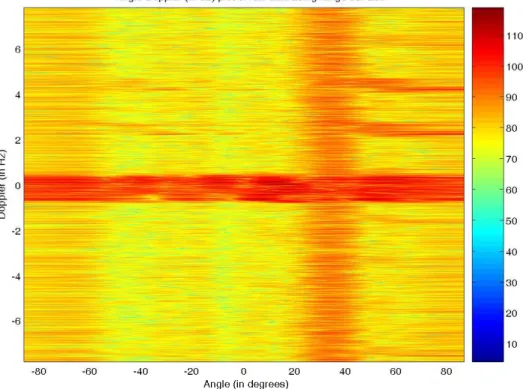
1.9 Angle-Doppler power distribution for range bin 50 . . . 15
1.10 Angle-Doppler power distribution for range bin 100 . . . 17
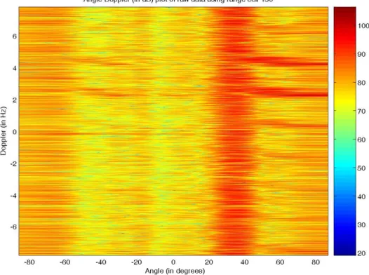
1.11 Angle-Doppler power distribution for range bin 150 . . . 17
1.12 Angle-Doppler power distribution for range bin 200 . . . 18
1.13 Angle-Doppler power distribution for range bin 225 . . . 18
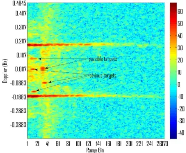
2.1 A range-Doppler plot of the data-square containing obvious targets. The targets are spread over up to 15 ranges and are at Doppler bins 89, 106, 131, and 151 respectively. . . 34
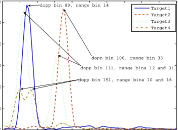
2.2 A power profile plot of the identified targets at Doppler bins 89, 106, 131, and 151 respectively. . . 35 2.3 Results of using the JDL and Nonadaptive algorithms to detect an ideal
target with amplitude 35 dB inserted into the ionospheric clutter region. 36
LIST OF FIGURES LIST OF FIGURES
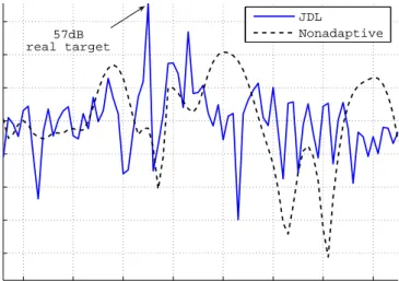
2.4 Results of using the JDL and Nonadaptive MF algorithms to detect a realistic target spread over 7 range cells and with amplitude 57 dB inserted into the ionospheric clutter region. . . 36 2.5 Results of using the hybrid, D3, JDL, and Nonadaptive MF algorithms to
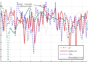
detect an ideal target with amplitude 55 dB inserted into the ionospheric clutter region. . . 38 2.6 Results of using the hybrid, D3, JDL, and Nonadaptive MF algorithms to
detect a realistic target spread over 7 range cells and with amplitude 55 dB inserted into the ionospheric clutter region. . . 38 2.7 Results of using the RSC-PAMF, TASC-PAMF, and Nonadaptive MF
algorithms to detect an ideal point target with amplitude 59 dB inserted into the ionospheric clutter region. . . 40 2.8 Results of using the RSC-PAMF, TASC-PAMF, and Nonadaptive MF
algorithms to detect a realistic target spread over 7 range cells and with amplitude 63 dB inserted into the ionospheric clutter region. . . 40
3.1 A tree-like representation of the FFA method for a datacube with M = 12 pulses, N = 12 elements, spatial-partitioning-sequence=[2,2,1,3], and temporal-partitioning-sequence=[4,1,3,1]. . . 45 3.2 A pictorial description of the Interleaved-FFA method. . . 50
4.1 Angle-Doppler plot of generated airborne data at range bin 223. . . 70 4.2 Probability of detection versus SNR for a PF A = 0.001 in the airborne
scenario using 3240 secondary samples. . . 72 4.3 Probability of detection versus SNR for a PF A = 0.001 in the airborne
scenario using 20 secondary samples. . . 72 4.4 ∆MSMI versus target amplitude for the JDL, and FFA algorithms using
K=93 secondary samples for covariance estimation. . . 74 4.5 ∆MSMI versus target amplitude for the JDL, and FFA algorithms in the
reduced sample support scenarios. . . 76 4.6 MSMI vs Range plots for using the AMF, and JDL methods. 6998
sec-ondary samples are used to estimate the covariance matrix. . . 79
LIST OF FIGURES LIST OF FIGURES
4.7 MSMI vs Range plots for using the Regular FFA, Interleaved FFA, and Randomized FFA methods. 6998 secondary samples are used to estimate the covariance matrix. . . 79 4.8 MSMI vs Range plots for using the AMF, JDL, and FFA methods. Only
20 secondary samples are used to estimate the covariance matrix. . . 80 4.9 MSMI vs Range plots for using the AMF, JDL, and FFA methods. Only
20 secondary samples are used to estimate the covariance matrix. . . 81 4.10 MSMI vs Range plots for using the Nonadaptive,and JDL methods to
detect a 45dB ideal target in Ionospheric clutter region. All 4096 pulses are used in this simulation. . . 83 4.11 MSMI vs Range plots for using the three FFA methods to detect a 45dB
ideal target in Ionospheric clutter region. All 4096 pulses are used in this simulation. . . 83 4.12 MSMI vs Range plots for using the Nonadaptive,and JDL methods to
detect a 45dB ideal target in Ionospheric clutter region. Only 128 pulses are used in this simulation. . . 85 4.13 MSMI vs Range plots for using the three FFA methods to detect a 45dB
ideal target in Ionospheric clutter region. Only 128 pulses are used in this simulation. . . 85 4.14 MSMI vs Range plots for using the Nonadaptive,and JDL methods to
detect a 45dB real target in Ionospheric clutter region. All 4096 pulses are used in this simulation. . . 87 4.15 MSMI vs Range plots for using the three FFA methods to detect a 45dB
real target in Ionospheric clutter region. All 4096 pulses are used in this simulation. . . 87 4.16 MSMI vs Range plots for using the Nonadaptive, and JDL methods to
detect a 45dB real target in Ionospheric clutter region. Only 128 pulses are used in this simulation. . . 88 4.17 MSMI vs Range plots for using the three FFA methods to detect a 45dB
ideal target in Ionospheric clutter region. Only 128 pulses are used in this simulation. . . 88
LIST OF FIGURES LIST OF FIGURES
4.18 ∆ MSMI versus Sequence Ranking in the airborne scenario for a 30dB ideal target using the regular FFA method for a sample support size of 20 secondary samples. . . 90 4.19 Total number of unit spatial and temporal partition lengths versus
Se-quence Ranking in the airborne scenario for a 30dB ideal target using the regular FFA method for a sample support size of 20 secondary samples. 91 4.20 Average MSMI versus Range plot, obtained by averaging the randomized
FFA detection results for a 35dB target over 10000 iterations. . . 92
A.1 An example of a 3×3 Localized processing region in the angle-Doppler domain of the JDL method. . . 99 A.2 Block diagram of the unconstrained Wiener Filter. . . 112 A.3 Block diagram of the general sidelobe canceler. . . 112 A.4 Block diagram of a 4 stage unconstrained Multistage Wiener Filter. . . . 115 A.5 Block diagram of the combined filterbank interpretation of the Multistage
Wiener Filter. . . 115
List of Abbreviations
ACE . . . Adaptive Coherence Estimator AMF . . . Adaptive Matched Filter AR . . . Auto Regressive
ASD . . . Adaptive Subspace Detector CFAR . . . Constant False Alarm Rate CNR . . . Clutter-to-Noise Ratio CPI . . . Coherent Processing Interval D3 . . . Direct Data Domain
DoF . . . Degrees of freedom
DRDC . . . Defense Research and Development Canada DSTO . . . Defense Science and Technology Organization EEZ . . . Exclusive Economic Zone
EM . . . Electromagnetic FFA . . . Fast Fully Adaptive FFT . . . Fast Fourier Transform
GLRT . . . Generalized Likelihood Ratio Test GSC . . . Generalized Sidelobe Canceller HF . . . High Frequency
HFSWR . . . High Frequency Surface Wave Radar JDL . . . Joint Domain Localization
JNR . . . Jammer-to-Noise Ratio km . . . kilometer
LPR . . . Local Processing Region
LIST OF FIGURES 2
MA . . . Moving Average
MSMI . . . Modified Sample Matrix Inversion MVDR . . . Minimum Variance Distortionless Filter MWF . . . Multistage Wiener Filter
NHD . . . Non-Homogeneity Detector nmi . . . Nautical Mile
OTHR . . . Over the Horizon Radar
PAMF . . . Parametric Adaptive Matched Filter PRF . . . Pulse Repetition Frequency
PRI . . . Pulse Repetition Interval RMB . . . Reed, Mallet, and Brennan sec . . . second
SINR . . . Signal-to-Interference-plus-Noise Ratio SNR . . . Signal-to-Noise Ratio
STAP . . . Space-time adaptive processing WF . . . Wiener Filter
Chapter 1
Introduction
Space-time adaptive processing (STAP) for airborne radar is a well studied area which has accumulated a substantial literature cache spanning more than 30 years. Although it was the early 1970’s that witnessed the inception of STAP through the pioneering work of Reed, Mallet, and Brennan [1], it was largely ignored for almost a decade due to the technological barriers of the time. STAP research has received a significant amount of interest recently, and, consequently, has undergone much progress.
The motivation for this thesis stems from the fact that the majority of the focus of the STAP literature has been on enhancing target detection in the airborne radar scenario. Little, if any, effort has been invested in the development of STAP techniques tailored to meet the specific needs of other interference environments. In particular, a literature survey of the available STAP techniques, indicated that no STAP method has been developed for high frequency surface wave radar (HFSWR) systems. Performance of target detection algorithms, especially non-adaptive techniques, in HFSWR, are primarily limited by sea clutter (at the near ranges) and ionospheric clutter (at the far ranges). In this regard, STAP appears to be a promising approach to deal with such interference.
This thesis has been undertaken in the context of a collaboration effort between the University of Toronto and the Defense Research and Development Canada (DRDC). The goal of this joint effort was the development of practical space-time adaptive processing schemes for HFSWR systems. In this thesis we use the operational DRDC HFSWR system as the source of the test system parameters. In addition, DRDC has provided us
1.1. MOTIVATION 2
with measured HFSWR data to test the algorithms developed in this work1.
A significant challenge in developing STAP for HFSWR is that traditional STAP algo-rithms invariably assume the interference to be spatially homogeneous, i.e., the statistics of the interference are consistent as a function of range. STAP algorithms exploit this homogeneity to estimate interference statistics for interference suppression. Specifically these statistics are estimated by averaging over the homogeneous range cells (referred to as homogenous ranges). Sea and ionospheric clutter, on the other hand, are well known to be highly non-homogeneous, requiring the development of alternative STAP approaches. However, as will be demonstrated through a preliminary analysis of the measured ionospheric clutter data sets, the fundamental limiting factor is the lack of a sufficient number of secondary range cells to estimate the interference statistics.
In this work, we evaluate the performance of several conventional STAP methods in the HFSWR scenario. We also develop a new reduced complexity multistage STAP approach, which we refer to as the Fast Fully Adaptive (FFA) approach.
1.1
Motivation
High frequency surface wave radars (HFSWR) naturally lend themselves to marine surveillance applications, and have several advantages that make them desirable for coastal surveillance applications. In particular they have large coverage area capabilities (over the horizon and beyond the exclusive economic zone (EEZ)), the lowest operating cost per unit coverage area of any radar system, as well as minimal operator interven-tion requirements [2]. These characteristics make HFSWR very desirable for low cost medium accuracy monitoring of low altitude aircraft and surface vessels with a cover-age span as far as and beyond the EEZ. The numerous advantcover-ages associated with the HFSWR setup, and the lack of adequate and practical HFSWR interference suppression methods, motivated our research into the development of more effective means of clut-ter mitigation for this specific inclut-terference environment. Thus although nonadaptive and one-dimensional (space or time only) adaptive ionospheric clutter suppression algorithms
1Another aspect of this effort was the development of an effective data model for HFSWR. However
1.2. SYSTEM AND DATA MODELS 3
have been developed, they are characterized by high complexity and a large dependence on the assumed model used to describe the ionospheric clutter [3]. This thesis, therefore, focuses on the development of low complexity STAP interference cancelation techniques for HFSWR systems.
1.2
System and Data Models
In this introductory chapter, we focus on the system and data models, and present the results of some preliminary, non-adaptive, processing of HFSWR data. This chapter sets the stage for adaptive processing of HFSWR data presented in Chapter 2.
Although our primary focus will be on the HFSWR scenario, we will also evaluate the performance of the FFA algorithm in the airborne radar setup. This will allow for a fuller characterization of this new multistage adaptive processing scheme. We are therefore interested in two primary radar setups: airborne surveillance radar, and HFSWR. Both these system models will be described in the following subsections. The system and data models described here will also allow us to place the available STAP literature in context. We begin with the airborne radar system model, which allows us to review the avail-able STAP literature.
1.2.1
Airborne Radar System Model
Airborne radar refers to the setup where the transmit and receive antennas are mounted onto an aircraft (for example on the side of an airplane) and used to scan the ground for targets amid a background of ground and/or sea clutter that might vary rapidly. For the airborne radar scenario we will adopt the conventional STAP setup, as developed in detail by Ward in [4].
Consider a side-looking equispaced linear array2 comprised of N isotropic, point sen-sors separated by a distance of λ/2, receiving an incident plane wave, as shown in Fig-ure 1.1. Each channel receives M data samples corresponding to the M pulses in a
1.2. SYSTEM AND DATA MODELS 4
Broadside
φ
x
d
Figure 1.1: A linear array of point sensors .
Figure 1.2: A 3 dimensional representation of a datacube.
coherent processing interval (CPI). Thus over the span of one CPI, the N channels pro-gressively collect NM space-time measurements composed of a mixture of the imping-ing target returns (if present) as well as background clutter, interference, and receiver noise. Upon dividing each pulse repetition interval (PRI) into L separate ranges the corresponding space-time snapshots at each range are compiled into one N × M ×L
data-cube (Figure 1.2). For each range bin, the received data can be stored in a length
NM vectorx whose entries numberedmN to [(m+ 1)N −1] correspond to the returns at the N elements from pulse number m, (m = 0,1, . . . , M −1). This data vector is a sum of the contributions from external interference sources, thermal noise and possibly a target, and can be written as,
1.2. SYSTEM AND DATA MODELS 5
where v represents a normalized target signature signal, c the vector of interference sources and n the thermal noise. ξ is the target amplitude and is zero under the null hypothesis (i.e., no target present).
Referring to Figure 1.2, the primary range cell refers to the range cell being tested for the presence of a target, while the secondary range cells refer to the neighboring ranges that will be used to estimate the interference covariance matrix. This interference covariance matrix will play a central role in the computation of the optimal adaptive weights in the adaptive matched filter (AMF) solution, which are used to suppress the unwanted interference and enhance the hidden target.
The vector vin Eqn. (1.1) is the space-time steering vector corresponding to a target at look angle φt and look Doppler frequency ft. This steering vector can be written in
terms of a spatial steering vector a(φt) and a temporal steering vector b(ft) [4],
v = b(ft)⊗a(φt), (1.2) a(φt) = £ 1 ej2πfs ej(2)2πfs . . . ej(N−1)2πfs¤T, (1.3) b(ft) = £ 1 ej2πft/fR ej(2)2πft/fR . . . ej(M−1)2πft/fR¤T , (1.4) fs = d λ sinφt, (1.5)
where ⊗ represents the Kronecker product of two vectors,T represents the transpose
operator, fs the normalized spatial frequency,λ the wavelength of operation and fR the
pulse repetition frequency (PRF). Eqn. (1.5) assumes the angle φt is measured with
respect to broadside (Figure 1.1).
The term c in Eqn. (1.1), refers to the interference and includes the effects of clutter and possible jammers. Ground clutter, the dominant form of clutter in airborne radar, is spread across range, azimuth, and Doppler and constitutes the major source of undesir-able interference in airborne radar. The Doppler spread associated with ground clutter is primarily due to the relative motion between the aircraft and the ground below. In [4],
1.2. SYSTEM AND DATA MODELS 6
ground clutter is modeled as the sum of the radar echoes from concentric clutter rings centered about the vertical projection of the aircraft onto the ground.
The other major source of interference in the airborne radar setup is barrage jamming, which refers to a jamming signal that is spatially correlated from element to element (i.e., behaves as a point target in space), and is temporally uncorrelated from pulse to pulse (i.e., behaves like thermal white noise temporally). A more detailed description and model of ground clutter and barrage jamming is available in Appendix A.1.
The final source of interference is the omnipresent thermal white Gaussian noise, which is uncorrelated from element to element and pulse to pulse.
The three interference sources can be lumped together into a single additive colored noise term.
Ideally a target (when present) is localized to one range bin, however in real systems the radar ambiguity function (defined formally in Eqn. (22) of [4]) leads to a spread of the target over several ranges, and this spread must be accounted for in the target model. In order to ensure an accurate estimate of the interference covariance, several (typically 2 or 3) guard ranges on either side of the primary range are used to prevent target influence from corrupting the estimate of the interference statistics. For simplicity however, we will assume that all airborne radar targets are ideal point targets, localized in range, azimuth, and Doppler.
1.2.2
HFSWR System Model
To overcome the primary source of propagation loss, namely sea surface roughness, HF-SWR are operated at relatively low frequencies of the High Frequency (HF) band (be-tween 2 and 6 MHz). One of the primary concerns with HFSWR is their high per-formance degradation due to highly non-homogeneous reflections from the ionospheric layer (termed ionospheric clutter). Although not the only source of unwanted signals,
1.2. SYSTEM AND DATA MODELS 7
the ionosphere plays a vital role in determining the performance of HFSWR based sys-tems. However unlike ground clutter in the airborne radar setup, ionospheric clutter in the HFSWR scenario is significantly more difficult to model. This is mainly due to the highly nonstationary characteristics of the ionosphere which vary widely with time of day, season, temperature, and location. The ionosphere is a highly ionized plasma layer of the atmosphere that spans from around 50km to about 400km above the surface of the earth. The primary source of ionization is ultraviolet radiation from the sun, which strips electrons from the neutral gas molecules leading to the formation of positive ions. The free electrons have affects on the propagation of electromagnetic (EM) radiation; in particular radio wave propagation. The level of ionization and the electron density are functions of both elevation and solar radiation intensity. As a result the electron density of the ionosphere, and consequently the characteristics of the ionospheric clutter, vary with elevation as well as time of day, season, and sun-spot activity.
There are two available data models for ionospheric clutter [3,6]. The work of Ravan et al. detailed in [7] indicated that the model proposed by Fabrizio [3], although analytically appealing, can not be used to model the measured ionospheric data acquired by the DRDC HFSWR. A more accurate model is developed by Riddolls [6, 8] which extends the model introduced by Coleman [9, 10], by simultaneously accounting for group delay, direction of arrival, location, and Doppler. The author uses a ray tracing model and treats irregularities as perturbations of a “quiescent” path solution without irregularities. This model has been recently implemented by Ravan [7].
Although ionospheric clutter is the dominant clutter source in the far ranges, it is sea clutter, and in particular the Bragg component of the sea clutter that dominates the near ranges. Sea clutter is characterized by a nonzero Doppler signature that is spread over the frequencies in the vicinity of the zero Doppler frequency; it exhibits particularly
1.3. PRELIMINARY DATA ANALYSIS: MEASURED DATA 8
strong returns at the Bragg Doppler frequencies given by,
fBragg=±
r g
πλ (1.6)
where g = 9.8m/s is the gravitational acceleration, and λ is the wavelength of the radar signal. The Bragg component is due to the constructive interference of radar echoes from ocean waves with a wavelength equal to λ/2 [11]. It should be noted that this Bragg clutter line begins to recede with increasing range, and almost disappears completely for ranges beyond 200km [12].
Having briefly introduced the types of clutter encountered in HFSWR, we next turn our attention to the target model used in this setup. Ideal targets in the HFSWR scenario can be modeled (quite accurately) in a fashion similar to targets in airborne applications (i.e., point sources localized in azimuth, Doppler, and range), and as a result we will use the conventional space-time steering vector, developed in the airborne radar literature [4], and summarized in Section 1.2.1, to model target returns in HFSWR. However in order to account for the spread of the target in range we will also use a realistic target space-time vector which is spread over several range bins, and extracted from measured high signal-to-noise-ratio (SNR) target returns present in separately measured HFSWR data cubes. We will have more to say on this subject later on.
1.3
Preliminary Data Analysis: Measured Data
This section details the non-adaptive data processing conducted on the data sets provided by DRDC, and used in our evaluation of several reduced complexity STAP techniques in the HFSWR scenario. In particular we will restrict our discussion in this section, to the analysis of the data set hfswr data 25mar2002 030257.mat.
1.3. PRELIMINARY DATA ANALYSIS: MEASURED DATA 9
sets used for the HFSWR simulations in this work. The reader is referred to [12] for a detailed description of the measurement setup. The measured ionospheric clutter was obtained above Cape Race in Newfoundland located on Canada’s East coast using a HF-SWR system operated by DRDC. The radar operates at a carrier frequency of 3.1 MHz. The data was obtained using a 16 element linear array with inter-element separation of 33.33m (corresponding to 0.344λ), and gathered over a time period of 4.37 minutes, divided into 4096 pulses with an effective pulse repetition frequency (PRF) of 15.625Hz (setting the maximum resolvable Doppler frequency to±7.8125Hz). The range span was about 400km divided into 270 consecutive range cells each covering a span of 1.5km. It should be noted that the measured data we received was oversampled in range by a fac-tor of approximately 4, which means that consecutive ranges were correlated to a certain degree. This correlation in range has a negative impact on the accuracy of the estimate of the interference covariance in the AMF solution, which requires that the secondary ranges used in the covariance estimate to be independent.
The data analysis conducted in this section focuses on non-adaptive processing, and is used to characterize the measured data set. Some sample results are provided illustrating the interference distribution as a function of angle, Doppler and range.
1.3.1
Element-Range Plots
The first set of results focus on the range dependence of the interference. Figure 1.3 plots the power distribution, in dB, of the first pulse as a function of element and range. There appears to be three distinct segments in range - a near range segment extending up to approximately range cell 50 with significant interference power, a segment between range cell 50 and 180 with lower power, and finally, the range cells dominated by ionospheric clutter past range cell 180. Figure 1.4, corresponding to pulse number 2000, reconfirms this impression.
1.3. PRELIMINARY DATA ANALYSIS: MEASURED DATA 10 50 100 150 200 250 2 4 6 8 10 12 14 16 Range # Element #
Element−range power (in dB) for pulse # 1
−10 0 10 20 30 40 50
Figure 1.3: Element-range power distribution for pulse number 1
50 100 150 200 250 2 4 6 8 10 12 14 16 Range # Element #
Element−range power (in dB) for pulse # 2000
−10 0 10 20 30 40 50
1.3. PRELIMINARY DATA ANALYSIS: MEASURED DATA 11
attenuated by as much as 40dB. This same problem exists in all the data-sets given to us by the DRDC. However, interestingly, focusing on this one element suggests that this receiver is not totally “dead”. The associated angle-Doppler plot in Fig. 1.7, presented later, has the appropriate characteristics, only they are attenuated by as much as 40dB.
1.3.2
Range-Doppler Plots
This section focuses on range-Doppler plots for individual elements. The Doppler domain is ‘accessed’ by performing a Fourier transform on the available pulses at each range for a specific element. Figures 1.5 and 1.6 plot the power distribution of the radar signal returns as a function of range and Doppler. As is clearly seen, there are three distinct clutter regions; the near region extending to approximately 140km (comprising approximately the first 50 range bins) dominated by the Bragg lines and sea clutter, a region at the far ranges beyond 330km dominated by the ionospheric clutter and, interestingly, a middle region of sea clutter with less structure. This corroborates with our initial impression from Figs. 1.3 and 1.4. As we will see in later plots, this variation in clutter structure is also visible in the angle-Doppler plots presented in Section 1.3.3 and has significant implications for interference suppression.
In both plots the Bragg lines are clearly visible. The advancing and receding lines are at ±0.18Hz corresponding to the expected Doppler frequency given by Eqn.( 1.6). An interesting conclusion can be drawn by plotting the range-Doppler power distribution for element 13 (Fig. 1.7). While our initial understanding was that channel 13 was “dead”, Fig. 1.7 reveals that in fact this channel appears to be receiving data, but attenuated by as much as 40dB with respect to the other elements.
These range-Doppler plots provide crucial information for the STAP process. As we will see in Chapter 2, a fundamental limitation of STAP is the need for training data to estimate the statistics of the interference within a primary range cell. This training data, clearly, must be statistically homogeneous with respect to the range cell under test. The
1.3. PRELIMINARY DATA ANALYSIS: MEASURED DATA 12
Doppler in Hz
Range in km
Range Doppler power plot (in dB) for element number 1
−0.8 −0.6 −0.4 −0.2 0 0.2 0.4 0.6 0.8 100 150 200 250 300 350 400 450 65 70 75 80 85 90 95 100
Figure 1.5: Range-Doppler power distribution for element number 1
Doppler in Hz
Range in km
Range Doppler power plot (in dB) for element number 8
−0.8 −0.6 −0.4 −0.2 0 0.2 0.4 0.6 0.8 100 150 200 250 300 350 400 450 70 75 80 85 90 95 100 105
1.3. PRELIMINARY DATA ANALYSIS: MEASURED DATA 13
Doppler in Hz
Range in km
Range Doppler power plot (in dB) for element number 13
−0.8 −0.6 −0.4 −0.2 0 0.2 0.4 0.6 0.8 100 150 200 250 300 350 400 450 30 35 40 45 50 55 60 65
1.3. PRELIMINARY DATA ANALYSIS: MEASURED DATA 14
range-Doppler plots indicate that there is limited training available within each clutter region. This is independent of whether the clutter is actually homogeneous within each of the three clutter regions described above.
1.3.3
Angle Doppler Plots
In this subsection we will analyze the angle-Doppler plots for individual range cells. These plots are useful since they illustrate the power distribution in angle-Doppler space; the two Fourier spaces corresponding to the spatial and temporal domains in which STAP will be implemented. It is well accepted that it is easier to suppress localized interference (localized near a specific Doppler/angle). We will see that the range cells dominated by the Bragg lines and those dominated by the ionospheric clutter appear to have a more coherent structure.
Figures 1.8 and 1.9 plot the angle-Doppler structure for range bins 1 and 50 re-spectively (ranges of 62.75km and 136.25km respectively). As is clear from Fig. 1.8 the interference in the first range bin has a clear structure - the Bragg lines near zero Doppler are visible across all angles. Also, the interference is localized to a few angles. We are also able to identify two major sources of discrete interference : (i) a high power interference source spread over all range and Doppler, and localized in azimuth (24◦-46◦). This source
has a coherent structure and we therefore believe it to be a communication channel; (ii) a high power interference source spread over all ranges, and localized in Doppler (4Hz and 2Hz) and azimuth (60◦-90◦), including two relatively strong source at approximately
35o (relative to broadside). As we will see, these two interference sources appear in all
range cells.
Figure 1.9 plots the power distribution in angle and Doppler for range cell 50, at the edge of the first interference region. Comparing this plot to Fig. 1.8 one can visualize the loss of structure in the interference. The interference here is far more spread out. This effect is further illustrated in Figs. 1.10 and 1.11 corresponding to range bins 100 and
1.3. PRELIMINARY DATA ANALYSIS: MEASURED DATA 15
Figure 1.8: Angle-Doppler power distribution for range bin 1
1.4. THESIS OVERVIEW 16
150. In these two figures the lack of structure in the clutter is particularly striking. This has significant implications for the STAP process; with its focus on a localized region in angle-Doppler space, an algorithm such as the joint domain localized (JDL) processing scheme [13, 14] may be useful here.
In the range cells dominated by ionospheric clutter, a structure is again visible in the angle-Doppler space. Figures 1.12 and 1.13 illustrates the strong ionospheric interference close to zero-Doppler and the external interference is again clearly visible.
In summary, the angle-Doppler plots suggest both the potential of STAP to suppress interference and also some cautionary tales. As our preliminary analysis of the HFSWR data revealed, the data cube appears to have three distinct regions. In the first region, dominated by the Bragg lines, a clear structure is visible and a “traditional” adaptive algorithm such as the sidelobe canceler followed/preceded by Doppler processing may be adequate. In the third region, dominated by ionospheric clutter, STAP is required due to the inherent non-stationarity of the clutter. In the middle region, again dominated by sea clutter, no structure is visible and a JDL-based algorithm might be required.
1.4
Thesis Overview
The remainder of this thesis is organized as follows; Chapter 2 reviews STAP and several STAP algorithms and presents simulation results that are used to evaluate the per-formance of these methods in HFSWR systems. Chapter 3 introduces the Fast Fully Adaptive approach as well as three different variants. The fast adaptive matched filter is also developed in this chapter by integrating the FFA approach into the optimal adap-tive matched filter (AMF). Chapter 4 presents several simulation results of applying the FFA algorithm to detect ideal and realistic targets in the airborne and HFSWR setups. Chapter 5 wraps up the thesis with some conclusions and several suggestions for future research in the context of the FFA and STAP for high frequency (HF) radar systems.
1.4. THESIS OVERVIEW 17
Figure 1.10: Angle-Doppler power distribution for range bin 100
1.4. THESIS OVERVIEW 18
Figure 1.12: Angle-Doppler power distribution for range bin 200
Chapter 2
Processing of HFSWR Returns
The central goal of this thesis is the development and analysis of practical STAP schemes for HFSWR radar systems. Our preliminary analysis of the dataset suggested that the most important issue with the available data is (a) the non-stationarity of the clutter and (b) the lack of sufficient secondary data to estimate the space-time covariance matrix. In this regard, of special interest are adaptive schemes that address clutter non-homogeneity and algorithms with fewer degrees of freedom. Examples of such algorithms include the Joint Domain Localized (JDL) algorithm [14], the direct data domain (D3) algorithm [15] and the combination of the two into the hybrid algorithm [16]. Other algorithms of interest are the parametric adaptive matched filter (PAMF) [17], and multistage Wiener filter (MWF) [18, 19]. The D3 and hybrid algorithms were designed specifically for non-homogeneous clutter, while the JDL, PAMF, and MWF were designed to address the issue of limited sample support.
As an initial step in this direction, we will begin by reviewing the basic concepts of STAP through a description of the optimal fully adaptive processor (also referred to as the adaptive matched filter (AMF)). Next we will briefly review some of the available adaptive processing techniques used in HFSWR. We will then turn our attention to the primary subject of this Chapter; applying low-complexity STAP to the HFSWR setup.
2.1. REVIEW OF FULLY ADAPTIVE STAP 20
Particularly we will review each of the JDL, D3, hybrid, PAMF, and MWF algorithms, and discuss the various advantages and drawbacks associated with each method, as well as how each of these schemes fits into the HFSWR setup. Finally, we will present several simulation results that will allow us to examine the effectiveness of STAP techniques in suppressing ionospheric clutter.
2.1
Review of Fully Adaptive STAP
In this section we will review fully adaptive STAP, and describe the advantages and drawbacks associated with the optimal solution. This optimal processor is of particular interest to us as it will form the main building block of the fast fully adaptive method we will develop in Chapter 3. Since STAP is strongly rooted in airborne surveillance radar, we will use the airborne system model, described in Section 1.2.1, to present the STAP techniques of interest to us in this work.
In this section we are concerned with the linearly constrained minimum variance distortionless response (MVDR) Wiener filter (WF), also referred to as the the matched filter (MF). The received signal vector can be written as,
x=ξv+n (2.1)
where ξ is the target amplitude, v is the target space-time steering vector at the angle and Doppler of interest, and n is the total colored interference.
STAP applies a set of weights, w, to this received data vector to form a statistic,
y=|wHx| (2.2)
where a target is declared present if y is greater thann a chosen threshold, and absent otherwise. The threshold, choice of weights, and interference environment determine the
2.1. REVIEW OF FULLY ADAPTIVE STAP 21
probabilities of detection and false alarm.
Assuming a data model where all the interference signals are zero mean, jointly sta-tionary, complex Gaussian processes, the MVDR-WF, is known to be the optimal adap-tive processor under the maximum signal to interference plus noise ratio (SINR) criterion. Under the Gaussian assumption the maximization of the probability of detection can be shown to be equivalent to the maximization of the SINR [20]. Thus under the assumption ofa priori knowledge of the interference statistics, and as a result of the error covariance matrix R, the matched filter solution leads to the computation of the following optimal weight vector,
wopt =R−1v, (2.3)
where R = E©nnHª is the known interference covariance matrix. This is also the
matched filter solution under colored noise.
Unfortunately, it is seldom the case that the interference statistics are known priori, and thus must be estimated from the neighboring ranges. This leads to an alternate suboptimal solution called the Adaptive Matched Filter (AMF), or the fully adaptive processor, which is identical to the WF with the known covariance R replaced by its maximum likelihood estimate Rb given by,
b R= 1 K K X r=1 xkxHk (2.4)
where xk is the space-time data snapshot at the kth secondary range cell. We can then
evaluate the following modified sample matrix inversion (MSMI) statistic [21],
ΛAM F =
¯ ¯
¯vHRb−1x¯¯¯2
vHRb−1v . (2.5)
2.2. LITERATURE REVIEW OF HFSWR PROCESSING TECHNIQUES 22
alarm rate (CFAR) independant of R. The false alarm rate is a function of N, M, and
K only.
Clearly the fully adaptive processor assigns an adaptive weight to each of the NM
degrees of freedom (DoF). However for the estimate Rb, of the interference covariance matrix to be accurate, the number of statistically homogeneous range cells used to pro-duce this estimate must be at least 2NM according to the Reed-Mallet-Brennan (RMB) rule [1]. Unfortunately such generous sample support is rarely available in practice (and is even more rare in the HFSWR scenario), leading to the computation of an inaccurate estimate of the true interference statistics. As seen in Chapter 1, while N = 16, and
M = 4096, we only have 93 range cells(¿than the 2NM = 131072 secondary ranges re-quired by the RMB rule) within the ionospheric region, a quarter of which are redundant due to the oversampling of the measured data in range. It is, therefore, the requirement of statistically homogeneous sample support that is fundamentally impossible to meet in practice. In addition, the computation of the optimal weight vector, involves the evalu-ation of the matrix inverse of Rb, which leads to an impractical computational load (in the order of (NM)3) for most practical choices ofM and N .
2.2
Literature Review of HFSWR Processing
Tech-niques
This section reviews some of the previously published work in adaptive processing for HFSWR. Largely the work appears to have focused on the reduction of the degrees of freedom (DoF) in the processing scheme so as to reduce computational load and the requirements of statistically stationary sample support.
Some of the early works by researchers at DRDC include [22, 23] which discuss the use of horizontal dipoles as auxiliary antennas to take on the role of sidelobe cancelers1,
2.2. LITERATURE REVIEW OF HFSWR PROCESSING TECHNIQUES 23
used in the suppression of skywave interference. The author derives the adaptive weights to optimally suppress interference. A reference signal is added to obtain the weights using a Wiener solution. In [24] the author extends the results [22, 23] to include a comparison between the use of horizontal and vertical dipoles for interference suppression. The author suggests the use of horizontal polarization to cancel interference close to the target location (whose signal is vertically polarized). This work may not have significant impact on the present project since all the antennas, used to obtain the measured data, use the same (vertical) polarization. Furthermore, these works adaptively process the space dimension only.
Other efforts within the DRDC include the coherent sidelobe canceler of [25], where the authors investigate the optimal ordering of Doppler processing, beamforming, and interference cancelation. One unfortunate result is that the optimal ordering is inter-ference dependent, and consequently time dependent, since the interinter-ference sources in HFSWR demonstrate a large variability with time. A similar result was demonstrated in the context of airborne radar in [13]. In [25], the sidelobe canceler is shown to be effective against a single spatially confined source. An interesting, and sobering, contri-bution in this paper is the demonstration of the wide spatial and temporal variation in the ionospheric clutter characteristics.
These works would, we believe, be considered “classical” in the space-time adaptive processing community, and underline the complexity of the problem being tackled in this project.
A significant fraction of the work in adaptive processing for HFSWR is apparently led by Dr. Yuri Abramovich and Dr. Giuseppe Fabrizio at Defense Science and Technology Organization (DSTO) in Australia [3, 26–30]. In particular, Fabrizio has several contri-butions developed in detail in his thesis and then several later works that are reviewed
High sidelobes are undesirable since they allow interference to leak into the output of the array. A sidelobe canceler is an adaptive processor used to reduce the sidelobe level.
2.2. LITERATURE REVIEW OF HFSWR PROCESSING TECHNIQUES 24
below. The work of Abramovich focuses largely on the underlying phenomenology and measurements [31].
The work of the group led by Fabrizio [3, 26–30] has focused on the development of the adaptive coherence estimator (ACE) and its variant, the spatial adaptive subspace detector (ASD) [26], for over-the-horizon (OTH) radar systems. In the following we largely focus on their most recent contributions [28–30] presented as an improvement on their previous work [3, 26, 27].
The ACE test, like the modified sample matrix inversion (MSMI) statistic, has the important CFAR property. However ACE has the CFAR property even when the data within the range cell under test has a different scale from that in the secondary data. Unfortunately, ACE is highly susceptible to target mismatch and hence the motivation for the development of the ASD detector.
The ASD detector treats a single target as a signal subspace with rank greater than 1 [29]. In their latest work [30], Fabrizio et al. address the issue of unwanted signals in the primary data. They propose a generalized likelihood ratio test (GLRT) to address this issue. To address the issue of target mismatch, they model both the target and the discrete interference source within the primary range cell as low-rank sources given by a linear combination of closely spaced Doppler frequencies. The GLRT is then formed by maximizing over the parameters of both the target and discrete interference. Unfor-tunately, a significant drawback is that the implementation of the GLRT requires exact knowledge of the parameters of the interference. This necessitates a two-pass approach wherein the detector acquires some knowledge of the existence of the interference and its parameters in real time. This two-pass approach is reminiscent of the two-pass approach proposed by Adve et al. in [32, 33]. It should be noted that other than the experimental results, the formulation in [30] does not specifically target HFSWR.
2.2. LITERATURE REVIEW OF HFSWR PROCESSING TECHNIQUES 25
authors developed a STAP algorithm [28] for OTH radar using beamspace-range2 pro-cessing. This paper is of interest because the authors claim that withN spatial elements and M time taps, they can reduce the dimension of the STAP filter to (M + N) as opposed to the usual MN. The move to beamspace is similar to the JDL scheme’s ap-proach of working in azimuth-Doppler space, in that the spacing between beams is not restricted to the use of a FFT. Interestingly, the authors usefast time samples3 pulses to form the Doppler steering vector, as opposed to the traditional slow time samples - hence the name beamspace-range processing.
The other significant group of researchers working in adaptive processing for HF radar is in China. In [34] the authors propose a scheme for clutter mitigation that both varies the clutter weights to counter non-stationary ionospheric clutter within a coherent processing interval (CPI) while maintaining some stability in the gain on target. Two issues with this paper appear to be the need for partitioning the overall CPI into sub-CPIs, increasing the computation load, and the somewhat ad-hoc nature of the proposed processing scheme with transitions from sub-CPI to sub-CPI.
The work in [35] is the basis for experimental results reported in [36]. In [35] the authors claim that clutter and target returns only impact the positive frequencies; and not the negative frequencies, however the basis for this claim is not clear to us.
In [37] the authors extend temporal only processing to the use of STAP. However, the approach used is the classical STAP (elaborated on in the previous section) approach of estimating the covariance using secondary data without any specific attention paid to homogeneity.
2For the special case of a uniform linear array, the beamspace domain can be accessed through a
Fourier transform of the spatial domain.
3The fast time samples refer to the range samples corresponding to a certain pulse, while the slow
time samples refer to the sequence of returns across all the pulses of a coherent processing interval corresponding to a certain range.
2.3. REVIEW OF LOW COMPLEXITY STAP TECHNIQUES 26
2.3
Review of Low Complexity STAP Techniques
In Section 2.1 we reviewed the fully adaptive processor. Although it provides the optimal solution, it is highly impractical due to its large sample support requirements, and its large computational load. To address these issues researchers have developed techniques that are characterized by a lower-complexity, and that utilize fewer adaptive DoF. Some popular low complexity approaches, developed in the context of airborne radar, include, the Joint Domain Localized (JDL) algorithm [14, 38], the Parametric Adaptive Matched Filter (PAMF) [17] and the reduced rank Multistage Wiener Filter(MWF) [18, 19]. In the following sections we will briefly describe several such low-complexity approaches. The details of the algorithms are left to Appendix A.2.
2.3.1
Joint Domain Localized (JDL) Processing
One popular low complexity STAP scheme is the JDL algorithm which was first proposed in [13] with strict constraints on the algorithm and generalized in [14] to eliminate these constraints and allow for the use of real-world antenna arrays with mutual coupling. The JDL processor adaptively processes the received data in the angle-Doppler domain, i.e., after transforming the received space-time data to the angle-Doppler domain. This transformation is accomplished by an inner product with a set of space-time steering vectors, i.e., the data at azimuth angle φ and Doppler frequency f is given by
ˆ
x=vH(φ, f)x, (2.6)
wherex is the measured space-time data at a specific range cell, and ˆxrepresents angle-Doppler data. Choosing a set ofηa angle and ηd Doppler bins centered at the look
angle-Doppler forms the data set, in the angle-angle-Doppler domain, used for adaptive processing. This set of ηa angle and ηd Doppler bins is said to form the Localized Processing Region
2.3. REVIEW OF LOW COMPLEXITY STAP TECHNIQUES 27
(LPR). Unfortunately, there is no known criteria for optimally choosing the spacings in angle and Doppler; in most implementations the optimal spacings have been found empirically [7]. The primary advantage of the JDL approach is the fact that only ηa
angle and ηd Doppler bins are used in the adaptive process with values in the range of 3
- 11 each. Significantly reducing the adaptive DoF in this manner yields corresponding reductions in required sample support and computation load. Appendix A.2.1 describes the JDL algorithm in more detail.
Despite the benefits of working in the angle-Doppler domain, the performance of the JDL algorithm, like all statistical algorithms, depends on the accuracy of an estimated interference covariance matrix. This in turn places homogeneity constraints on the in-terference. Unfortunately this constraint is often violated in practice, and more so in the case of high-power clutter returns from the ionospheric layer, which are characterized by their inherent inhomogeneity, presence of discrete-like clutter sources, and variability. However, if the various parameters that characterize the ionospheric clutter have a co-herence time longer than several CPIs, and are coupled with the use of algorithms such as JDL, the detrimental effect of the inhomogeneities may be minimized [39].
The essential cause of this problem is the dependence of the algorithm on the statis-tics of the interference. Alternative, deterministic, adaptive approaches to suppress in-homogeneous clutter, have been developed to solve this problem. One notable class of deterministic algorithms are the so-called direct data domain (D3) algorithms. Examples of this class of algorithms are the one-dimensional D3 algorithm, as developed in [16,40], and the two-dimensional (D3) of [41]. We will describe the one-dimensional D3 algorithm in the next subsection.
2.3.2
D
3and Hybrid Approaches
The D3 algorithm, developed in [16] and improved upon in [40], is a purely non-statistical algorithm which does all its processing using only the primary range cell without relying
2.3. REVIEW OF LOW COMPLEXITY STAP TECHNIQUES 28
on the neighboring ranges to extract an estimate of the interference covariance matrix. As a result the D3 algorithm is immune to both clutter non-homogeneities in the secondary data and target-like, discrete, interference sources within the primary range cell. The discrete interference may occupy multiple angle and Doppler bins. This scenario is more relevant to us since the ionosphere, with its highly nonhomogeneous nature, is expected to resemble, to a certain degree, a source of high power discrete interference spread over numerous range cells leading to a contamination of the homogeneity of the secondary data.
The D3 algorithm computes an adaptive weight vector that does not rely on the computation of an error covariance matrix. It first forms a temporal residual matrix, At,
free from any target returns by subtracting the returns from all the consecutive pulses after appropriate scaling. It then selects a temporal weight vector that maximizes the signal-to-interference-plus-noise ratio (SINR):
ˆ wt= arg max wt ¯ ¯wH t b(ft) ¯ ¯2 ||AH t b(ft)||2 . (2.7)
The solution results from solving a generalized eigenvalue problem [40]. After forming a similar spatial weight vector, ˆws using the data from the spatial domain, the final
space-time weight vector is given by w = ˆwt⊗wˆs. A more rigorous description of the
one-dimensional D3 algorithm is available in Appendix A.2.2.
In the DRDC data sets, M = 4096, making the matrix in question singular. Even finding the generalized eigenvalues becomes difficult since the algorithms involved become unstable. However this problem can be overcome by adding a small diagonal loading to the matrix.
The drawback of the D3 approach is that by focusing exclusively on the data within a single range cell, it completely ignores all useful correlation information. Since iono-spheric clutter is a mix of correlated and discrete interference, the performance of the D3
2.3. REVIEW OF LOW COMPLEXITY STAP TECHNIQUES 29
algorithm is inadequate. One other disadvantage of the D3 algorithm is that it requires the computation of the inverse of an (M −1)×(M −1) matrix which can be quite a daunting task when the number of pulses is large. To overcome some of the weaknesses of the D3 method, the hybrid algorithm was developed in [16]. The hybrid is a two-stage algorithm whose building blocks are the D3 and JDL algorithms, respectively. It uses the D3 weights as an adaptive transform to the angle-Doppler domain. The angle-Doppler data for angle φ and Doppler f is given by
ˆ
x=wH(φ, f)x, (2.8)
wherew(φ, f) is the D3 adaptive weight vector corresponding to angleφ and Doppler f. Choosing ηa angle and ηd Doppler bins forms the LPR for the JDL algorithm. During
the statistical adaptive processing stage, the JDL nulls the correlated interference by computing a weight vector derived from the estimate of the error covariance matrix in the transformed domain. Thus the hybrid algorithm is capable of suppressing both uncorrelated and correlated interference in the target range, and as a result theoretically performs better than both the JDL and D3 algorithms. We provide a more detailed description of the hybrid algorithm in Appendix A.2.3.
2.3.3
Parametric Adaptive Matched Filter (PAMF)
Another reduced-domain algorithm that shows robustness to the presence of hetero-geneous interference in the target range, is the Parametric Adaptive Matched Filter (PAMF) algorithm [17]. The underlying principle is the use of linear estimation theory to obtain an estimate of the inverse of the error covariance matrix, but using fewer com-putation cycles than the conventional AMF method. PAMF is based on the block-LDL decomposition of the covariance matrix, R, where the non-zero block elements of the
2.3. REVIEW OF LOW COMPLEXITY STAP TECHNIQUES 30
autoregressive (AR) process of order p, whose error covariance matrix is the p-th block matrix of the block diagonal matrix D. Since R is not known a priori, the coefficients of L and D must be approximated by assuming the underlying process is a P-th order multichannel AR process and using an appropriate parameter estimation algorithm to estimate the coefficients of this multichannel AR(P) process. An excellent discussion of multichannel AR processes and several corresponding parameter estimation techniques are available in [42]. A more detailed description of the PAMF algorithm is available in Appendix A.2.4.
It is claimed in [17] that the PAMF method also shows robustness to the presence of discrete interference in the secondary data and has performance that rivals that of the MF even in the case of limited sample support. Unfortunately the PAMF method is not CFAR (i.e., the false alarm rate varies with the interference level), however simulation results suggest that for certain PAMF configurations CFAR like behavior does occur [17]. The main drawback of the PAMF is difficulty associated with the selection of an optimal AR order and the complexity of its implementation. Although the authors in [17] claim that an AR order of 3 is sufficient to accurately model the underlying process in airborne radar, no such investigation has been conducted in the HFSWR case which may very well require a much higher AR order given the highly nonhomogeneous nature of the ionospheric clutter. Another issue with the PAMF is its larger implementation complexity as compared to other available low complexity methods such as the JDL and D3. A final drawback of using the PAMF is that it lacks the CFAR property. Although simulation results in [17] indicate that for certain configurations the PAMF does yield CFAR like behavior, this is not a general rule of this algorithm and as a result reduces the practicality of the PAMF to a certain extent.
2.4. APPLYING STAP TO HFSWR 31
2.3.4
Multistage Wiener Filter (MWF)
The multistage Wiener filter (MWF) developed in [18,19] is an equivalent representation of the optimal Wiener filter that admits a recursive decomposition into a series of scalar Wiener. We defer the description of the MWF to Appendix A.2.5. This decomposition eliminates the need of directly working with the full MN ×MN covariance matrix, and instead only deals with the computation of numerous scalar Wiener Filter weights. Although this might seem as a huge advantage, especially for large values of the product
MN, the complexity reduction gained by eliminating the need for computing the inverse of a large dimensional matrix, is regained through the large number of matrix products and error signal recombinations constituting the analysis and synthesis stages of the MWF. One solution to this complexity problem comes in the form of the reduced rank MWF where the decomposition is interrupted at thePthstage [18]. This can be achieved
by discarding the last (NM −1−P) rows of the analysis filterbank matrix, L. One justification for this is that the covariance of the observed data tends to become white as the number of stages increases, and therefore a close approximation to the optimal Wiener filter can be obtained by truncating the P ‘deepest’ stages where the vector hk
approaches 0 [18]. However this reduced rank solution might still be impractical in the HFSWR case where the product MN is extremely large. Another solution to the large complexity associated with the MWF, and without reverting to a reduced rank filter, can be obtained by incorporating the conjugate gradient method into the MWF [43].
2.4
Applying STAP to HFSWR
In the previous sections we reviewed the optimal fully adaptive filter and several sub-optimal, reduced complexity STAP methods. All the described methods can be directly applied to the HFSWR setup under the assumption of an interference environment whose
2.4. APPLYING STAP TO HFSWR 32
statistics are sufficiently homogeneous across range so as to allow for an acceptable es-timate of the covariance to be obtained. The assumption of a Gaussian interference environment would also allow retaining the CFAR properties of the MSMI statistic used in the AMF, JDL, hybrid, and MWF methods. Unfortunately the ionospheric clutter is known to be a form of highly inhomogeneous and nonstationary interference. However over shorter periods of time, we hope that the ionospheric clutter maintains enough ho-mogeneity over the secondary ranges used in the covariance estimation, so as to render the STAP methods, discussed in the previous section, useful. We will therefore assume a sufficiently stationary and homogeneous environment with complex Gaussian interfer-ence statistics, and use the results of the STAP simulations to verify the validity of this simplifying assumption.
To perform the simulations, we use the measured dataset, described in Section 1.3. Our primary focus will be the assessment of how effectively STAP can mitigate iono-spheric clutter. As a result we will mainly focus on the ranges dominated by ionoiono-spheric clutter, namely range cells 176 to 270. The fully adaptive processor, although optimal, is inapplicable to our test setup. The reason for this is two-fold; first the minimum required sample support, as dictated by the RMB rule, is K = 2MN = 2(4096)(16) = 131072 secondary samples, and only 94 ionospheric clutter range cells are available; second the computational load associated with estimating and inverting the 65536×65536 covari-ance matrix is beyond the capabilities of most modern processors. We must therefore direct our efforts towards the more practical, albeit suboptimal, approaches suggested in the previous section.
2.5. PERFORMANCE OF AVAILABLE STAP ALGORITHMS IN HFSWR 33
2.5
Performance of Available STAP Algorithms in
HFSWR
In this section we will attempt to evaluate the performance of the existing low-complexity STAP methods, described in Section 2.3, in the HFSWR setup. The simulation results to be presented in this section, will allow us to assess the level of utility of STAP in HFSWR applications.
We will begin by describing the realistic target model which takes the radar ambigu-ity function into account, and which will be used in addition to the ideal target model, described in Sections 1.2.1, and 1.2.2, to characterize the performance of the chosen algo-rithms. Next we will present several simulation results detailing the performance of these algorithms, followed by a ‘Discussions’ section where we will identify the implications of the simulation results.
2.5.1
Realistic Target Model
Assuming a point target model has several advantages such as simplicity, localization to a single range bin, and the elimination of the need to incorporate the ambiguity function into the target model. It also does have a role in characterizing the performance of the algorithm being tested. Unfortunately ideal targets do not exist in the real world and we must therefore choose a more realistic target model. To account for the spread of real targets in range we used obvious realistic targets directly extracted from a sample data-square (since only one spatial channel was used) provided to us by DRDC. Figure 2.1 shows a range-Doppler plot of this data-square where the targets are indicated by arrows. Note that the ideal target model does have a role to play in identifying the performance of the algorithms under test. Figure 2.2 shows several superposed cross-sections of the range-Doppler plot at the Doppler bins corresponding to some of the identified targets
2.5. PERFORMANCE OF AVAILABLE STAP ALGORITHMS IN HFSWR 34
Figure 2.1: A range-Doppler plot of the data-square containing obvious targets. The targets are spread over up to 15 ranges and are at Doppler bins 89, 106, 131, and 151 respectively.
present in the data-square. It should be noted that the range span of the data-square places it in the region dominated by Bragg lines and thus little or no ionospheric clutter masks the targets.
As can be seen from the plots in Figure 2.2 the realistic targets exhibit a range-power profile that extends over several range bins with the peak range-power located near the center of the target’s range span. In our simulations we will particularly focus on the targets located at Doppler−0.1526Hz (Doppler-bin 89) and−0.087Hz (Doppler-bin 106) respectively. It should be noted that we first normalized the targets by dividing by the magnitude of the peak target amplitude, and then dividing by the magnitude of the corresponding steering vector, before actually injecting the target at the desired angle and Doppler locations. A final yet important detail to note is that the magnitude of both the ideal and realistic targets used in the simulations are an absolute magnitude andnot a signal-to-noise ratio (SNR).
2.5. PERFORMANCE OF AVAILABLE STAP ALGORITHMS IN HFSWR 35 0 10 20 30 40 50 60 70 80 90 100 0 50 100 150 200 250 300 Range bin Abs(magnitude) dB Target1 Target2 Target3 Target4 dopp bin 89, range bin 14
dopp bin 151, range bins 10 and 16 dopp bin 131, range bins 12 and 31
dopp bin 106, range bin 35
Figure 2.2: A power profile plot of the identified targets at Doppler bins 89, 106, 131, and 151 respectively.
2.5.2
Simulation Results
In this section we provide some of the results obtained by using the algorithms described in the previous sections to detect ideal and realistic targets injected into the region dominated by ionospheric clutter. Both the ideal and realistic targets used were injected at an angle of 35◦ and a Doppler of 0.18Hz. The ideal target used is localized to a
single range bin, while the realistic target used is that extracted from the data-square at Doppler bin 89, and is spread over ranges approximately 7 ranges.
To assess the performance of the algorithms under investigation we focus on the peak MSMI at the target range and the difference in MSMI (in dB) between the peak MSMI and the second highest statistic, denoted as ∆MSMI. The larger the ∆MSMI the larger the capability of an adaptive algorithm to distinguish between a target and residual interference, and thus the better its performance. We begin by presenting some of the JDL algorithm results.
2.5. PERFORMANCE OF AVAILABLE STAP ALGORITHMS IN HFSWR 36 180 190 200 210 220 230 240 250 260 −20 −15 −10 −5 0 5 10 Range Bin MSMI statistic (dB) JDL Nonadaptive target
Figure 2.3: Results of using the JDL and Nonadaptive algorithms to detect an ideal target with amplitude 35 dB inserted into the ionospheric clutter region.
190 200 210 220 230 240 250 260 −20 −15 −10 −5 0 5 10 15 Range Bin MSMI statistic (dB) JDL Nonadaptive 57dB real target
Figure 2.4: Results of using the JDL and Nonadaptive MF algorithms to detect a realistic target spread over 7 range cells and with amplitude 57 dB inserted into the ionospheric clutter region.


![Figure 3.1: A tree-like representation of the FFA method for a datacube with M = 12 pulses, N = 12 elements, spatial-partitioning-sequence=[2,2,1,3], and temporal-partitioning-sequence=[4,1,3,1].](https://thumb-us.123doks.com/thumbv2/123dok_us/1926323.2783580/57.892.158.782.211.878/representation-datacube-elements-partitioning-sequence-temporal-partitioning-sequence.webp)