Score-Driven Models for Realized Volatility

Cambridge Working Papers in Economics: 1950

SCORE-DRIVEN MODELS FOR REALIZED VOLATILITY

Andrew Harvey Dario Palumbo

30 May 2019

This paper sets up a statistical framework for modeling realised volatility (RV ) using a Dynamic Conditional Score (DCS) model. It first shows how a preliminary analysis of RV, based on fitting a linear Gaussian model to its logarithm, confirms the presence of long memory effects and suggests a two component dynamic specification. It also indicates a weekly pattern in the data and an analysis of squared residuals suggests the presence of heteroscedasticity. Furthermore working with a Gaussian model in logarithms facilitates a comparison with the popular Heterogeneous Autoregression (HAR), which is a simple way of accounting for long memory in RV. Fitting the two component specification with leverage and a day of the week effect is then carried out directly on RV with a Generalised Beta of the second kind (GB2) conditional distribution. Estimating logRV with an Exponential Generalised Beta of the second kind (EGB2) distribution gives the same result. The EGB2 model is then fitted with heteroscedasticity and its forecasting performance compared with that of HAR. There is a small gain from using the DCS model. However, its main attraction is that it gives a comprehensive description of the properties of the data and yields multi-step forecasts of the conditional distribution of RV.

Cambridge Working Papers in Economics

Score-Driven Models for Realized Volatility

Andrew Harvey and Dario Palumbo

Faculty of Economics, Cambridge University

May 30, 2019

Abstract

This paper sets up a statistical framework for modeling realised volatility (RV ) using a Dynamic Conditional Score (DCS) model. It …rst shows how a preliminary analysis of RV, based on …tting a linear Gaussian model to its logarithm, con…rms the presence of long memory e¤ects and suggests a two component dynamic speci…cation. It also indicates a weekly pattern in the data and an analysis of squared resid-uals suggests the presence of heteroscedasticity. Furthermore working with a Gaussian model in logarithms facilitates a comparison with the popular Heterogeneous Autoregression (HAR), which is a simple way of accounting for long memory in RV. Fitting the two component speci…cation with leverage and a day of the week e¤ect is then carried out directly on RV with a Generalised Beta of the second kind (GB2) conditional distribution. Estimating logRV with an Exponential Gen-eralised Beta of the second kind (EGB2) distribution gives the same result. The EGB2 model is then …tted with heteroscedasticity and its forecasting performance compared with that of HAR. There is a small gain from using the DCS model. However, its main attraction is that it gives a comprehensive description of the properties of the data and yields multi-step forecasts of the conditional distribution of RV.

Keywords: EGARCH; GB2 distribution; HAR model; heteroscedas-ticity; long memory; weekly volatility pattern.

1

Introduction

This paper sets up a general model for realized variance (RV) based on a distribution that is coherent for non-negative variables. The dynamics

de-pend on the score of the conditional distribution. Score-driven models were developed in Harvey (2013) and Creal et al (2013) where they were called DCS and GAS models respectively. The contribution of this paper is to show how the score-driven approach provides an integrated framework for volatil-ity modeling and how its application to RV yields new insights, as well as giving forecasts which are as good as, if not better, than those obtained from existing techniques. As well as giving a comprehensive description of the properties of the data, it able to provide multi-step forecasts of the condi-tional distribution of RV.

A preliminary analysis of RV can be carried out by …tting a linear Gaussian model to its logarithm. (This has an additional attraction of yielding smoothed estimates of the underlying level of the series.) In our example, this analy-sis con…rms the two component speci…cation that has often been found in GARCH and EGARCH models and at the same time reveals a weekly pattern in RV. It also clari…es the relationship with the popular Heterogeneous Au-toregression (HAR) model, devised by Corsi (2009) and Müller et al (1997), which is a simple approximation to the high-order autoregression implied by long memory. Fitting the two component speci…cation is then carried out di-rectly on RV with a Generalised Beta distribution of the second kind (GB2) conditional distribution. The Burr, Pareto and log-logistic are all special cases of GB2 and the F distribution is closely related. These distributions have fat tails but the DCS model handles extreme values robustly. Estimat-ing a GB2 for RV is equivalent to estimatEstimat-ing a model for its logarithm with an Exponential GB2 (EGB2) distribution. The EGB2 provides further insights into the overall picture because it has the normal distribution as a limiting case. Furthermore it is easily extended to allow for heteroscedasticity.

Finally we comment on the relevance of our …ndings for the multivariate score-driven models for RV covariance matrices proposed by Opshoor et al (2016).

2

Statistical framework

This section sets out a coherent statistical framework for modeling RV that respects the non-negativity of the observations and the tendency of variance to increase with the level; see Corsi et al (2008) and Taylor (2005, p 335-7). When volatility is estimated from RV, it may be calibrated for returns by re-estimating the constant from the standardized returns assuming a

distri-bution, such as generalized-t. The resulting estimates of scale, or standard deviation, are then used to give forecasts based on the conditional distrib-ution of returns; compare Brownlees and Gallo (2006) or Harvey (2013, p 180-1).

2.1

Dynamic location/scale model

A dynamic location/scale model for a non-negative variable is

yt= t tpt 1; t= 1; :::T; (1) where the random variable t has unit mean. In the MEM model of

En-gle and Gallo (2006), the conditional mean, _{tpt 1}; follows a GARCH-type process and has to be constrained to be positive. Estimation is by maximum likelihood (ML), based on the conditional distribution, f(yt jYt 1).

An equivalent model can be formulated in terms of scale, tpt 1; in which case yt = "t tpt 1; where E("t); unlike E( t); is not equal to one, unless

the distribution is exponential. However, E("t) is easily found. With an

exponential link function for the scale,

yt="texp( tpt 1); t = 1; :::T; (2) where the logarithm of scale, tpt 1; is unconstrained. The structure is the same as that of EGARCH, as in Harvey (2013, chs 4 and 5) and Harvey and Lange (2017), and much of the theory is the same: hence the name Beta-GB2-EGARCH. First-order dynamics for tpt 1 take the form

t+1jt =!(1 ) + tjt 1+ ut; (3)

whereut is the score of the conditional distribution ofyt:As with EGARCH, j j <1ensures stationarity and there is no need to restrict parameters to be non-negative. When the distribution is fat-tailed, the score is bounded. This makes it possible to show the model is invertibility subject to restrictions on

.

Taking logarithms in (2) gives

lnyt=xt= tpt 1+ ln"t (4)

so tpt 1 now becomes location. A distribution for "t implies a

distribu-tion for ln"t; so the model can, in principle, be estimated in levels or logs.

Comparison of the likelihoods requires a Jacobian term to account for the transformation.

2.2

GB2 conditional distribution

The usual form of the GB2 density, as given in Kleiber and Kotz (2003, p.187) and Harvey (2013, ch 5), is

f(y) = (y= )

1

B( ; &) [(y= ) + 1] +&; ; ; ; & >0; (5)

where is the scale parameter, ; and & are shape parameters and B( ; &)

is the beta function. The standardized GB2, as it appears in (2), is

f("t) =

"_t 1

B( ; &) ["_t + 1] +&; ; ; & >0:

The score wrt the logarithm of scale is

@lnft @ tpt 1 =ut= ( +&)bt( ; &) ; (6) where bt( ; &) = (yte tpt 1) (yte tpt 1) + 1 ; t = 1; :::; T; (7) is distributed as beta( ; &); see Harvey (2013, ch 5). As y _{! 1}; the score approaches an upper bound of = &; whereas the lower bound of is obtained when y= 0:

Remark 1 The GB2 distribution can be reparameterized so that the (upper)

tail index, ; replaces &; that is we de…ne = &. The generalized gamma

(GG) is then obtained as a limiting case as _{! 1} by replacing by ' 1= _.

The Weibull is a special case of GG in which = 1 ( and a special case of

Burr as _{! 1}) while setting = 1 gives the gamma distribution. The

chi-square is a special case of standardized gamma and a limiting case of the F

distribution. The score for GG is unbounded and for gamma it isyte tpt 1

so the response is linear.

The asymptotic distribution of the ML estimator is given in Harvey (2013, ch 5). When, as is usually the case, is positive, a su¢ cient condition for the model to be invertible is that

< 4(1 + )₂

for all values in the parameter space; see Appendix.

Taking the logarithm of a GB2 gives the exponential GB2 (EGB2) dis-tribution. The EGB2 is symmetric when = &: It includes normal, when

= & _{! 1}; Laplace, when = & _! 0; and logistic, when = & = 1; see McDonald and Xu (1995) and Caivano and Harvey (2014).

Ify is distributed as GB2( ; ; ; &) and x= lny; the PDF of the EGB2 variate x is

f(x; ; ; ; &) = expf (x ) g

B( ; &)(1 + exp_f(x ) _g) +&: (9)

The logarithm of scale in GB2, that is ; becomes a location parameter in EGB2. Furthermore is now a scale parameter, but and & are still shape parameters and they determine skewness and kurtosis. The distribution has light (exponential) tails. All moments exist with the mean equal to +

1_{[ ( ) (&)]and the standard deviation given by =h= ; where h}2 ₌

0_{( ) +} 0_{(&); with and} 0 _{denoting the digamma and trigamma functions}

respectively. The distribution is positively (negatively) skewed when > &

( < &) and its kurtosis decreases as and & increase; excess kurtosis does not exceed six.

Although is a scale parameter in (9), it is the inverse of what would be considered a more conventional measure of scale. Scale is better de…ned as the standard deviation

=h= ; where h= q 0_{( ) +} 0_{(&); (10)} leading to ut = 2 @lnft @ = h[( +&)bt( ; &) ]; (11) where bt( ; &) = e(xt tpt 1)h= e(xt tpt 1)h= _{+ 1}; t = 1; :::; T: (12) Note that bt( ; &) is as in the GB2, that is (7), but with replaced by h=

and ytexp( tpt 1) replaced by exp(xt tpt 1): Hence the score is bounded as _jx_{j ! 1}:

The inclusion of 2 in (11) means that letting & = _{! 1} yields ut !

xt tpt 1 ; see Caivano and Harvey (2014). The DCS model is then the innovations form of the Kalman …lter for a Gaussian unobserved components

model, which in the …rst-order case, (3), is

xt = t+"t; t N ID(0;

2_{); t = 1; : : : ; T;}

t+1 = t+ t; t N ID(0;

2_);

whereN ID(0; 2_{)denotes normally and independently distributed with mean} zero and variance 2 _{and E(}

t s) = 0 for all t; s:

Although the invertibility constraint, (8), is often not restrictive in prac-tice, it clearly creates di¢ culties as and & become bigger. However, when

ut is de…ned as in (11), the invertibility condition is

h2( +&)=4 <1:

For a (log) logistic distribution, when = & = 1; the invertibility condition is _j 1:645 _j < 1: As & = _{! 1}; it is shown1 _{in the appendix that the}

standard invertibility condition for a Gaussian model is obtained, that is

j j<1; see Harvey (2013, p 67). When >0

< 4(1 + )

h2_{( +&)} (13)

which yields <1 + for the Gaussian model.

2.3

Dynamic components

Instead of capturing long memory by a fractionally integrated process, two components may be used. For RV (and range), the leverage term is governed by sgn( rt); where rt denotes mean-adjusted returns; see Harvey (2013, pp

178-9). Thus

tjt 1 = !+ 1;tjt 1+ 2;tjt 1; (14)

i;t+1jt = i i;tjt 1+ iui;t+ i sgn( rt) (ut+ 1); i= 1;2:

The score curve from the RV model is rotated and, when the distribution of (mean-adjusted) returns is symmetric, the expectation of the composite variable driving the dynamic equation is zero. Identi…ability requires _{1 6}= ₂;

together with 1 6= 0 or 1 6= 0 and 2 6= 0 or 2 6= 0: An attraction of the

1_{If & ! 1while remains …xed at a …nite value, establishing whether the model is}

two-component DCS model is that the leverage e¤ect can di¤er in the long and short run.

Other components may be added. Here we employ a seasonal component

tjt 1 so

tjt 1 = !+ 1;tjt 1+ 2;tjt 1+ tjt 1; (15) where _{tjt 1} is as in Harvey (2013, p 79-80), that is

tjt 1 = z0t tjt 1 (16)

t+1jt = tjt 1+ tut;

where zt picks out the current season. In season j we set j = ; where is

a non-negative unknown parameter, whereas i = =(s 1)for i6=j: The

amounts by which the seasonal e¤ects change therefore sum to zero. The …lter treating the elements of 1j0 as parameters. (There ares 1free parameters because they sum to zero.) In the present application the ‘seasons’are days of the (working) week, so s = 5: The exponential link function prevents the scale from becoming negative.

A random walk level can be extended so as to mirror an integrated random walk (IRW) in a UC model, that is

1;t+1jt = 1;tjt 1 + _{1;tjt 1}

1;t+1jt = 1;tjt 1 + ut:

In a Gaussian UC model the IRW yields a smooth trend when the Kalman …lter ans smoother (KFS) is applied.

2.4

Long memory, Fractional integration and HAR

The standard HAR model, as in Corsi (2009), takes the form

b yh;t+h = + dyt+ wyw;t+ mym;t+ h;t+h; (17) where yt is RV, yw;t = P5 i=1yt i=5 ; ym;t = P22 i=1yt i=22 and ybh;t+h is the h-day cumulative average for h = 1;2; :: Usually h = 1 in which case

b

yh;t+h =yt+1: The disturbance term is h;t+h: The coe¢ cients are estimated

by regression. The weekly and monthly averages approximate the kind of lag structure found with long memory and are seen a simple alternative to a fractionally integrated model.

Remark 2 In the reparametrization of Patton and Sheppard (2015) the model speci…cation has the second term consisting of only the realized volatilities be-tween lags 2 and 5, and the third term consisting of only the realized volatili-ties between lag 6 and 22. If the Patton and Sheppard parameters are denoted

with a star, then d = d+ (1=5) w+ (1=22) m; w = (4=5) w + (4=22) m

and _m = (17=22) _m: The sum of the coe¢ cients is the same.

As set up in (17), the HAR is a regression model for a variable that is intrinsically positive, with a standard deviation that, in a GB2 framework, is proportional to the location. Working in logarithms, particularly whenh= 1;

this stabilizes the variance2_{; see also Corsi et al (2008) and Corsi and Reno}

(2012). In this case the y_t0s in the summations of (17) are replaced by their logarithms. The fact that the model for logarithms, (4), is additive makes aggregation more appealing because the (conditional) variance is constant.

3

Data Description and preliminary analysis

The simplest estimator of RV in day t is

RVt = m

X

i=1

r2_t;i; t = 1; ::::; T;

where rt;i is the return in the i-th subperiod in the day; see, for example,

Andersen et al (2003). The current study uses RV based on high-frequency index transaction prices from FTSE 100, DAX, S&P 500 and NASDAQ. The dataset is the one used by Patton and Sheppard (2015) and is constructed from …ve-minute intraday returns in the Oxford Man Institute library3_{. The}

observations are for weekdays, with public holidays assumed to be the same as the previous day. The starting date, 3rd January 2000, corresponds to the …rst non-weekend/holiday date in the U.S. The end is May 23, 2017. The sample size is therefore T = 4536:

When ln"t in (4) is not too far from normality4, …tting a linear state

space model may be a convenient way of …nding a suitable speci…cation

2_{Weighted least squares (WLS), as used by Patton and Sheppard (2015), is better than}

OLS, but it still does not acknowledge that the conditional distribution cannot possibly be normal.

3_{We use the variable ‘rv5’from https://realized.oxford-man.ox.ac.uk.}

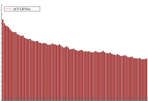
ACF-LRVftse 0 10 20 30 40 50 60 70 80 90 100 0.1 0.2 0.3 0.4 0.5 0.6 0.7 0.8 0.9 1.0 ACF-LRVftse

Figure 1: Correlogram of log of FTSE RV

for a dynamic model based on the conditional EGB2 distribution. This is easily done using the STAMP package of Koopman et al (2008). Smoothed estimates of volatility, that is estimates constructed from two-sided …lters, are readily available. Taking logarithms also facilitates a comparison with HAR.

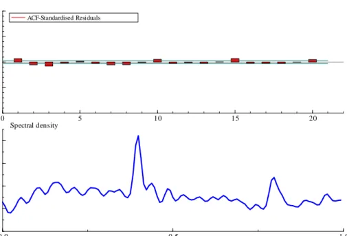
The preliminary analysis is carried out with FTSE RV, but the analysis of the other indices leads to similar conclusions. The …rst 23 observations were dropped so as to enable a comparison to be made with HAR. The long memory features are apparent in the ACF of its logarithm shown in Figure 1. Hence the decision to …t two components. In any case, …tting only one AR(1) component gives a very high portmanteau statistic, Q(67); at 410 and the …rst-order residual autocorrelation is also high at r(1) = 0:078: When two AR(1) components are included,r(1)reduces to 0.033, butQis still very high and correlations at lags of ten, …fteen and twenty (but not …ve) are apparent is negatively skewed and the excess kurtosis goes to six as _!0:Taking logarithms may be less appealing in such cases. A better option for QML is to model yt with a gamma distribution and a linear response function.

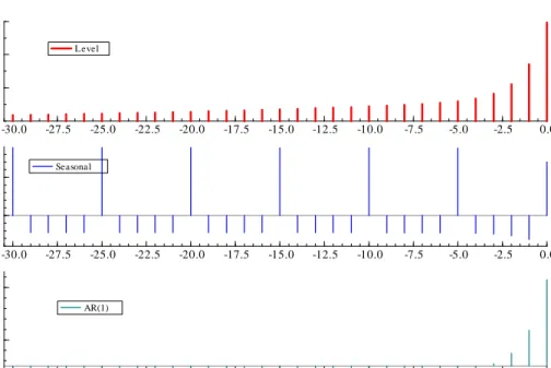
in the residual ACF shown in Figure 2. Furthermore the associated spectrum shows a clear peak at 2/5 and at its harmonic 4/5. Thus there is strong evidence for a day of the week e¤ect. The model is therefore augmented by including a weekly seasonal component as in (16). The seasonals appear to be …xed and the seasonal test statistic, which is asymptotically 25under the null of no seasonal e¤ect, is 203.2. The day of the week coe¢ cients are -0.132, -0.052, -0.002, 0.088 and 0.098. Thus Thursday and Friday exhibit much higher volatility than the other days, with Monday being particularly low5. The short-term component has a coe¢ cient of 0.75 which when combined with a long-run coe¢ cient close to unity implies a long memory pattern for the ACF. With the seasonal included, the implied weights in the …lter are as in Figure 3.

There is no evidence of …rst-order serial correlation as r(1) = 0:007 and although the 117.5 value for Q(70)is statistically signi…cant at conventional levels its value is not excessive given the large sample size. The only real failure of the model is in the distribution of the residuals: there is positive skewness and excess kurtosis of about 2.6.

The HAR model does rather well given its simplicity but Q(67) is high6

at 230.9 and the prediction error variance is 0.240 compared with 0.230 for the unobserved component model. The sum of the coe¢ cients is 0.96 and in the Patton-Sheppard form, the estimates of _d; _w and _m are 0.46, 0.38 and 0.12 respectively; compare the weights in Figure 3.

The Gaussian model allows smoothing. If the …rst component is modelled as an integrated random walk (IRW), that is

1;t+1 = 1;t+ 1;t; 1;t+1 = 1;t+ t;

the smoothed estimates are as shown in Figure 4.

4

Location/scale DCS model

Estimating a model with a conditional GB2 distribution with the parameters

; and can be problematic. We therefore focus on the Burr distribution,

5_{The realised measures in the Oxford library are explicitly constructed so as to ignore}

any extreme movements in the …rst few minutes of the trading day, which may be caused by large overnight volatility.

6_{This is only partly explained by the failure to take account of the day of the week}

ACF-Standardised Residuals 0 5 10 15 20 -0.5 0.0 0.5 1.0 ACF-Standardised Residuals 0.0 0.5 1.0 0.1 0.2 0.3 0.4 Spectral density

Figure 2: ACF and spectrum of residuals from …tting a RW and AR1 to

Level -30.0 -27.5 -25.0 -22.5 -20.0 -17.5 -15.0 -12.5 -10.0 -7.5 -5.0 -2.5 0.0 0.05 0.10 0.15 Level Seasonal -30.0 -27.5 -25.0 -22.5 -20.0 -17.5 -15.0 -12.5 -10.0 -7.5 -5.0 -2.5 0.0 0.0000 0.0005 Seasonal AR(1) -30.0 -27.5 -25.0 -22.5 -20.0 -17.5 -15.0 -12.5 -10.0 -7.5 -5.0 -2.5 0.0 0.1 0.3 AR(1)

Figure 3: Filter weights for linear Gaussian model for lnF T SErv

in which = 1; and what we call the balanced GB2 where = &: The log-logistic distribution is a special case of both Burr and balanced GB2 in which

& = = 1; whereas the generalized Pareto distribution is a special case of Burr with = 1:The logarithm of the balanced GB2 has a symmetric EGB2 distribution which, as noted earlier, goes to a normal distribution as ; & _{! 1}

meaning that the GB2 becomes lognormal. Finally the F-distribution with

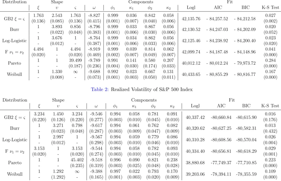
( 1; 2)degrees of freedom, is a special case of balanced GB2 in which = 1 and =& = 1=2 = 2=2;but more generally, ( 1= 2)F is GB2( 1=2; 2=2): Based on the speci…cation suggested by the preliminary analysis, we …t-ted these distributions with two autoregressive components. The Weibull is included for comparison. It is not a fat-tailed distribution, but like the lognormal, it can be obtained from GB2 as a limiting case. Table 1 shows the FTSE results, where, according to the AIC and BIC information crite-ria, Burr is best, whereas Table 2 for S & P 500 shows balanced GB2 to be better. The results for DAX and NASDAQ, which are available on request, show DAX leaning towards Burr and NASDAQ preferring balanced GB2. The estimate of & for FTSE is around 0:8 which implies positive skewness

LRVftse Trend 100 200 300 400 500 600 700 800 900 -12 -10 -8 -6 LRVftse Trend LRVftse-AR(1) 100 200 300 400 500 600 700 800 900 -1 0 1 2 LRVftse-AR(1)

Figure 4: Smoothed estimates when long-run component is an IRW and short-run component is an AR(1).

and excess kurtosis for the EGB2. The implied EGB2 values for excess kur-tosis and skewness are 2.76 and 0.54, which are close to the values for the residuals reported in the previous section.

The values of the tail indices are similar for all four markets, but tend to be lower for the Burr distribution. For example with FTSE the upper (lower) indices for Burr and balanced are 3.33 (3.89) and 4.48 (4.48) for balanced. The F-distribution does well, particularly when the balanced GB2 is best overall. The estimated in balanced GB2 is typically greater than one and the estimates of are& correspondingly smaller than those reported forF;as a result the tail indices are of a similar magnitude. In the log-logistic, where and& are constrained to be unity, it is that adjusts to give comparable tail indices. Although the …t of the log-logistic is good, the hypothesis that = 1

is rejected for all markets by Wald tests on the balanced GB2 estimates. The …t with distributions from the generalized gamma class, such as Weibull, is poor.

The Kolmogorov-Smirnov test is informative for comparing the distrib-utional …t. When a formal test is carried out at a nominal 5% signi…cance level, it tends to reject most of the distributions, an exception being the bal-anced GB2 for S&P. However, such rejections may not be surprising given the large sample size.

The low tail indices found in the best GB2 models indicate that the log-normal distribution gives an inferior …t and this is con…rmed by the goodness of …t statistics; for FTSE the log-likelihood is 42,067 which is well below the log-likelihood of 42,136 obtained for the balanced GB2 where = & = 1:76

rather than in…nity. For S&P, the lognormal log-likelihood is 40,312, again well below balanced GB2. The …t for Pareto is much worse than lognormal and like Weibull it is not considered further.

The seasonality does not show up clearly in residuals from …tting a non-seasonal location/scale model to levels, that is yt=exp( tjt 1). However, the ACFs of scores from the models reported in Tables 1 and 2 yield results similar to those for the ACF of the Gaussian UC model in Figure 2. This is because the scores for GB2 and EGB2 are the same and the Gaussian model is not too far away from a balanced EGB2 with moderate size tail indices.

The results in Table 3 show the parameter estimates for each index with the best-…tting distribution. The dynamic equation now includes a seasonal component and the two autoregressive components incorporate leverage ef-fects. Taking logarithms and …tting a corresponding EGB2 gives the same estimates and score residuals. The seasonal pattern is similar to that

re-ACF-T a ilSc ore 0 5 10 -0.5 0.0 0.5 1.0

ACF-T a ilSc ore ACF-absRe s 0 5 10 -0.5 0.0 0.5 1.0 ACF-absRe s

ACF-T woT ailSc ore

0 5 10

-0.5 0.0 0.5 1.0

ACF-T woT ailSc ore ACF-XiT a ilSc ore

0 5 10

-0.5 0.0 0.5 1.0

ACF-XiT a ilSc ore

Figure 5: FTSE: ACFs of scores for absolute values of residuals from preferred

lnRV model (top left hand) plus ACFs of scores for tail parameters.

vealed by the preliminary modelling and the leverage e¤ect is stronger in the short-term component, a …nding that is not unusual for returns or range; see Harvey and Lange (2018) and Harvey (2013, pp 176-81).

Table 4 shows the day of the week e¤ect. In all cases there is very little movement with the estimate of s being zero in three cases. For the US

indices the most volatile days are Wednesday and Thursday, whereas for the European indices it is Thursday and Friday.

5

Heteroscedasticity and a Changing Tail

In-dex

Although the residuals from the preferred Gaussian model have relatively little serial correlation, this is not true for their squares or absolute values: Figure 5 clearly indicates heteroscedasticity.

function, that is = exp( ); yields

@lnft=@ = ( +&)"tbt "t 1; (18)

where "t = (xt tjt 1)=exp( )and

bt=

exp"t

1 + exp"t

:

The score is symmetric but unbounded7; see Figure 2 in Caivano and Harvey (2014).

Parameterizing in terms of ln ; gives

@lnft=@ln =ut=h( +&) tbt h t 1; (19)

where t is (xt tjt 1)= ="t=h. Caivano and Harvey (2014, p 566) show

that in the limit as =& _{! 1}; ut= (xt tjt 1)2= 2 1;which is the score for a Gaussian EGARCH model. At the other extreme, when =& = 0; the score is p2 xt tjt 1 = 1:

How should heteroscedasticity in the logarithm of a variable that is al-ready subject to changing variance be interpreted? As was noted earlier, the (upper) tail index for a GB2 is = &:Thus for a …xed value of&;a dynamic implies that is dynamic. It also might imply that the lower tail index,

; is dynamic. We could let the tail indices be dynamic and keep …xed. Setting =& and letting& = exp( &) so& = ln&; gives

@lnft=@& = 2& (&) 2& (2&) &"t 2&ln(1 bt): (20)

This score is symmetric. Figure ?? compares @lnft=@& and @lnft=@ for

& = = 1:The response is similar in this case. If =& is not assumed,

@lnft=@& =& (&) & (&+ ) &ln(1 bt) (21)

and, as can be seen from the graph, the (dashed) curve is asymmetric with large positive (negative) observations lowering (raising) the value of&:Figure 5 shows that the ACF of this score, like that of the lower tail, gives little indication of any serial correlation8.

7_{Gen-t parameterized as in Harvey and Lange (2017) does have a bounded score for}

this parameter but tail index is …xed.

-5 -4 -3 -2 -1 1 2 3 4 5 -2 -1 1 2 3 4 x Score

Estimation of the GB2/EGB2 with a two component location/scale, sea-sonal dummies and dynamic ;captured by a …rst-order equation for tjt 1; gives the results shown in Table 5. In all cases apart from DAX, the dynamic e¤ects in t_jt 1 are short-lived with the AR coe¢ cient only slightly bigger than0:5. Nevertheless, the information criteria in Table 6 indicate that their inclusion improves the …t. Furthermore there is a big reduction in the value of the portmanteau statistis for ;but not by enough to completely eliminate the residual heteroscedasticity.

Remark 3 Corsi et al (2008) introduce heteroscedasticity into a model for logRV using GARCH combined with a normal inverse Gaussian distribution (NIG). The score-driven approach is more easily developed with EGB2 dis-tribution.

6

Forecasting

In order to compare the forecasting performance of the DCS models with the HAR model, we identi…ed two time periods of …ve months, one with large market ‡uctuations, labelled High Volatility Period, and one of relatively quiet market conditions, the Low Volatility Period. The High Volatility Pe-riod, between the 01/10/2008 and the 31/03/2009, covers the 2008 …nancial

crisis and includes the announcement of the bankruptcy of Lehman Brothers. The Low Volatility period is between the 01/02/2005 and the 29/07/2005. Models for each period were estimated using all the observations up to the beginning of the the period. Then one step ahead forecasts were computed for all the forecasting period.

The models compared are the location/scale DCS Seasonal EGARCH model, with and without heteroscedasticity (dynamic tjt 1), the HAR model in levels, as de…ned9 by Patton and Sheppard (2015), and the HAR model in logarithms, as de…ned by Corsi (2009). The one step ahead forecasts for the mean of the GB2 model are obtained by making a modi…cation to the forecast of the scale; see Harvey (2013, p163). In the general case with heteroscedasticity e yt+1jt = + 1= _T+1jT & + 1= _T+1jT ( ) (&) e t+1jt_{; t =T + 1; :::; T +T ;}

whereT denoted the number of observations in the forecasting period. When the HAR model is estimated in logarithms. In the latter case, the standard lognormal correction factor is used to give byT+1jT = exp xbT+1jT + ^2=2 .

In Table 7 the forecasting accuracy is measured in terms of Root Mean Squared Forecast Errors (RMSFE) and Mean Absolute Forecast Errors (MAFE) which are presented as percentages with respect to the standard DCS Sea-sonal EGARCH model. The signi…cance of di¤erences in forecasting accuracy is assessed from the p-values of the Diebold and Mariano (1995) test for equal expected loss of forecasts based on the proposed model versus each competi-tor. Finally, we have included the results for the predictive likelihood; see Mitchell and Wallis (2011).

The results in Table 7 show that the DCS model easily beats the HAR models according to predictive likelihood. This is what matters if we are concerned with the full distribution; see, for example, Corsi et al (2008, p 73). Comparisons based on RMFSE and MAFE are less clear cut: although DCS beats HAR in most cases, the di¤erences are rarely statistically signi…cant. In periods of Low Volatility the DCS forecasts better than the HAR on the European indices whereas for High Volatility regimes it forecasts better on the American indexes. In summary although HAR is generally di¢ cult to beat when the criterion is RMSFE or MAFE, the DCS model is certainly not

9_{They allow for heteroscedasticity by Weighted Least Squares, with weights given by}

worse and may be slightly better. What is clear, however, is that the HAR performs better when formulated in logarithms.

In all the cases the predictive likelihood is the highest for the DCS mod-els, always slightly in favour of the heteroscedastic EGB2 (DCS- tjt 1). As might be expected, HAR is much better in logarithms. This is because in levels the assumption of normality, even after removing the heteroscedastic-ity by weighted least squares, is still not a good one for observations which are strictly positive and skewed to the right (upwards) with a heavy upper tail. As was observed in Section 3, assuming normality for lnRV, thereby implicitly assuming thatRV is lognormal, is not unreasonable as an approx-imation.

In order to assess the relevance of accurately describing the predictive density, we looked at the upper quantiles. This is analogous to computing Value at Risk (VaR) for a return. For the DAX index, the Burr distribution gave the best …t and in this case the quantile function takes a particularly simple form, with the probability that RV is in the upper 100 % given by

u

e

yT+1jT = 1 exp T+1jT 1=& 1

1= T+1jT

: Comparing these quan-tile for = 0:10 and 0:25 with the corresponding quantiles for HAR (in logs), it seems that the HAR quantiles are consistently higher. This suggests an unreasonable hedge in a portfolio to protect against volatility risk and a tendency to overestimate a volatility spillover e¤ect in a systemic risk assess-ment. These are implications that go beyond the simple point forecast which has been extensively highlighted in the literature, and should be considered carefully by risk managers and policy makers.

Table 7 also includes results for the HAR-with-Jumps (HARJ) and Continuous-HAR (CContinuous-HAR) models proposed by Andersen et al. (2007). These are based on the idea that the total variation of RV can be decomposed into a contin-uous and discontincontin-uous component, that is a ‘jump’component. Following Barndor¤-Nielsen and Shephard (2004), this decomposition can be imple-mented through the Bi-Power Variation (BPV), de…ned as

BP Vt =zt =

2

M_X1

i=1

jrtij jrti 1j:

The series on BP V for the four indices come from the same Oxford Man Realized Library dataset as was used before. The CHAR model replaces RV by BPV in the right hand side of the levels HAR speci…cation, so that

y_h;t+h = + _dzt+ wzw;t+ mzm;t+ h;t+h: (22)

The HARJ model adds a jump variable, Jt = maxfyt zt;0g, to the

stan-dard HAR giving

y_h;t+h = + _dyt+ wyw;t+ mym;t+ JJt+ h;t+h: (23)

The performance of both CHAR and HARJ is dissappointing. Perhaps for-mulations designed for the logarithm of RV will fare better.

7

Conclusion

A location/scale DCS model for RV, formulated with a GB2 distribution in levels, or equivalently an EGB2 distribution in logarithms, is able to capture the mains features of the data. It is statistically coherent and can model long memory, through a two component structure, and asymmetric response (leverage) in a straightforward and transparent manner. The asymptotic theory for the ML estimator is as in Harvey (2013, ch 5), but here we show an additional result which indicates that invertibility for models with parameters that tend to arise in practice is unlikely to be a problem.

Working in logarithms is useful in that the normal distribution is a lim-iting case of EGB2 and preliminary investigation is easily carried out using linear state space models. ForRV data on the four indices FTSE, DAX, S&P and Nasdaq, preliminary analyis reveals a day of the week pattern, as well as long memory e¤ects. The more general score-driven models can handle these e¤ects and are able to introduce leverage into both short and long run components. The best …tting distributions are found to be the Burr and the balanced GB2, where the two shape parameters are set equal, resulting in a symmetric distribution for lnRV and a normal distribution as a limiting case. Both Burr and balanced GB2 both have only two parameters in addi-tion to those required to model dynamic locaaddi-tion/scale. The F-distribution also gives a relatively good …t to RV, even though it is not the best. How-ever, it does generalize the most easily to the modelling of anN N realized volatility covariance matrix as in Opschoor et al (2017).

Heteroscedasticity, or Volatility of Volatility (‘Vol of Vol’) as described by Corsi (2008), is detected in lnRV and can be modeled within the frame-work of an EGB2 distribution. We note that such heteroscedasticity implies dynamic tail indices in the corresponding GB2 distributions.

The forecasting performance of the models was assessed using HAR as a benchmark. HAR performs much better in logarithms than in levels, because in levels it fails to match the empirical distribution of the residuals. The point is worth stressing because some researchers, such as Patton and Sheppard (2015) and Bollerslev, Patton and Quaedvlieg (2016), continue to make a case for modeling in levels. When formulated in logarithms, the HAR model forecasts well, but it rarely beats the the DCS model in terms of RMSE or MAE. Furthermore the DCS model captures the conditional distribution more accurately. The di¤erence is re‡ected in the upper quantiles, and we argue that this may have implications for risk management; compare the use of score-driven models proposed by Lucas et al. (2016) for forecasting implied default probabilities in Credit Default Swap (CDS) prices.

References

Andersen, T.G., Bollerslev, T. and Diebold, F.X. (2010), "Parametric and Nonparametric Volatility Measurement," in L.P. Hansen and Y. Ait-Sahalia (eds.), Handbook of Financial Econometrics. Amsterdam: North-Holland, 67-138.

Andersen, T.G., Bollerslev, T., Diebold, F., Labys, P. (2003). Modeling and Forecasting Realized Volatility. Econometrica, 71, 579-625.

Audrino, F. and F. Corsi (2010) Modeling tick-by-tick realized correla-tions. Computational Statistics and Data Analysis 54, 2372-2382.

Barndor¤-Nielsen, O.E. and Shephard, N., 2002. Econometric analysis of realized volatility and its use in estimating stochastic volatility models. Journal of the Royal Statistical Society, Series B, 64, 253–280.

Blasques, F., Gorgi, P., Koopman, S.J. and O. Wintenberger (2018). Fea-sible invertibility conditions and maximum likelihood estimation for observation-driven models. Electronic Journal of Statistics, 12, 1019-1052.

Bollerslev, T., Patton, A.J., and Quaedvlieg, R. (2016). Exploiting the errors: A simple approach for improved volatility forecasting. Journal of

Econometrics, 192, 1-18.

Caivano, M. and A.C. Harvey (2014). Time series models with an EGB2 conditional distribution. Journal of Time Series Analysis, 34, 558-71.

Corsi, F., Mittnik, S., Pigorsch, C., and U. Pigorsch (2008). The volatility of realized volatility. Econometric Reviews, 27, 46-78.

Corsi, F. and R. Reno (2012). Discrete-Time Volatility Forecasting With Persistent Leverage E¤ect and the Link With Continuous-Time Volatility Modeling, Journal of Business and Economic Statistics, 30, 368-80.

Creal, D., Koopman, S. J. and A. Lucas (2013). Generalized autoregres-sive score models with applications. Journal of Applied Econometrics, 28, 777-95.

Engle, R. F. and G. M. Gallo (2006). A multiple indicators model for volatility using intra-daily data. Journal of Econometrics 131, 3-27

Harvey, A.C. (2013). Dynamic Models for Volatility and Heavy Tails:

with applications to …nancial and economic time series. Econometric Society

Monograph, Cambridge University Press.

Harvey, A.C. and R-J. Lange (2017). Volatility Modelling with a Gener-alized t-distribution, Journal of Time Series Analysis, 38, 175-90

Harvey, A.C. and R-J. Lange (2018). Modelling the Interactions between Volatility and Returns. Journal of Time Series Analysis, 39, 909–919.

Kleiber, C. and S. Kotz (2003). Statistical Size Distributions in

Eco-nomics and Actuarial Sciences. New York: Wiley.

Koopman, S. J. Harvey, A. C., Doornik, J. A. and N. Shephard (2009).

STAMP 8.2 Structural Time Series Analysis Modeller and Predictor.

Lon-don: Timberlake Consultants Ltd.

Lucas, A., Schwaab, B. and X. Zhang (2014). Conditional Euro Area sovereign default risk. Journal of Business and Economic Statistics,32, 271-84.

McDonald J. B. and Y. J. Xu (1995) A generalization of the beta distri-bution with applications. Journal of Econometrics 66, 133-152.

Mitchell, J. and K. F. Wallis (2011). Evaluating density forecasts: fore-cast combinations, model mixtures, calibration and sharpness. Journal of

Applied Econometrics 26, 1023-1040.

Muller, U., M. Dacorogna, R. Dav, R. Olsen, O. Pictet, and J. von Weiz-sacker (1997). Volatilities of di¤erent time resolutions – Analysing the dy-namics of market components. Journal of Empirical Finance 4, 213–239.

Opschoor, A, Janus, P., Lucas, A. and D J. van Dijk (2018). New HEAVY Models for Fat-Tailed Realized Covariances and Returns,Journal of Business

and Economic Statistics, 36, 643-7.

Patton, A. J. and K. Sheppard (2015). Good Volatility, Bad Volatility: Signed Jumps and the Persistence of Volatility. Review of Economics and

Statistics, 97, 683–697.

Taylor, S. (2005). Asset Price Dynamics, Volatility, and Prediction. Princeton University Press.

Appendix on invertibility Let

t( ) := supjxtj;

where xt =d t+1jt=d tjt 1 = + (@ut=@ tpt 1): Blasques et al (2018) show that a su¢ cient condition for invertibility is Eln 0( )<0 over all admissi-ble : For GB2 @ut @ tpt 1 =u0_t= 2( +&)bt(1 bt): Thus xt= + u0t= 2_{( +&)b} t(1 bt)

The maximum ofbt(1 bt) is1=4and so the model is invertible if we ensure

2_{( +&)=4 <1 (24)} Hence 4(1 ) 2_{( +&)} < < 4(1 + ) 2_{( +&)}

These bounds appear to place a constraint on the magnitude of and

&: However, this di¢ culty can be avoided by analysing the EGB2 with the forcing variable de…ned as in (11). Then

2@t2lnft

@ 2_{tpt 1} =h

2_{( +&)b}

t(1 bt)

and since the maximum of bt(1 bt) is again 1=4; the invertibility condition

is

h2( +&)=4 <1;

compare (24). For a logistic distribution, when =& = 1; the invertibility condition is _j 1:645 _j < 1: As & = _{! 1}; the distribution becomes normal and since, as noted in Caivano and Harvey (2014, Lemma 1, p 560),

&h2 = h2 _!2;it follows that h2( +&)=4_!1and the standard invertibility condition for a Gaussian model is obtained, that is _{j j} < 1; see Harvey (2013, p 67).

1. Tables

Table 1: Realized Volatility of FTSE 100 Index

Distribution Shape Components Fit

ξ υ ς ω φ1 κ1 φ2 κ2 Logl AIC BIC K-S Test

GB2ξ =ς _(0.136)1.763 _(0.085)2.543 _(0.136)1.763 _(0.415)-8.827 _(0.001)0.999 _(0.007)0.036 _(0.040)0.842 _(0.006)0.058 42,135.76 - 84,257.52 - 84,212.58 _(0.002)0.027 Burr 1 3.893 0.856 -8.796 0.999 0.033 0.867 0.056 42,130.52 - 84,247.03 - 84,202.09 0.020 - (0.022) (0.048) (0.383) (0.001) (0.006) (0.030) (0.006) (0.052) Log-Logistic 1 3.676 1 -8.764 0.999 0.034 0.862 0.056 42,125.46 - 84,238.92 - 84,200.40 0.023 - (0.012) - (0.387) (0.001) (0.006) (0.033) (0.006) (0.020) Fν1=ν2 4.494 1 4.494 -8.919 0.999 0.039 0.814 0.062 42,099.74 - 84,187.48 - 84,148.96 0.041 (0.020) - (0.020) (0.469) (0.002) (0.007) (0.049) (0.007) (0.000) Pareto 1 1 39.499 -9.789 0.991 0.141 0.580 0.207 40,012.12 - 80,012.24 - 79,973.72 0.284 - - (0.187) (0.236) (0.004) (0.030) (0.174) (0.033) (0.000) Weibull 1 1.330 ∞ -9.688 0.992 0.023 0.667 0.131 40,433.65 - 80,855.29 - 80,816.77 0.167 - (0.008) - (0.073) (0.001) (0.003) (0.050) (0.011) (0.000)

Table 2: Realized Volatility of S&P 500 Index

Distribution Shape Components Fit

ξ υ ς ω φ1 κ1 φ2 κ2 Logl AIC BIC K-S Test

GB2ξ=ς _(0.220)3.234 _(0.126)1.450 _(0.220)3.234 _(0.277)-9.546 _(0.003)0.994 _(0.010)0.058 _(0.045)0.781 _(0.010)0.091 40,337.42 -80,660.84 -80,615.90 _(0.176)0.016 Burr 1 3.271 0.798 -9.617 0.994 0.061 0.762 0.082 40,320.62 -80,627.25 -80,582.31 0.013 - (0.023) (0.048) (0.287) (0.003) (0.009) (0.047) (0.009) (0.432) Log-Logistic 1 2.997 1 -9.567 0.994 0.059 0.779 0.086 40,310.28 -80,608.56 -80,570.04 0.026 - (0.012) - (0.298) (0.003) (0.010) (0.046) (0.010) (0.004) Fν1=ν2 3.153 1 3.153 -9.544 0.994 0.058 0.782 0.093 40,334.40 -80,656.81 -80,618.29 0.029 (0.020) - (0.020) (0.274) (0.003) (0.010) (0.045) (0.010) (0.001) Pareto 1 1 45.402 -9.518 0.996 0.090 0.821 0.238 38,880.68 -77,749.37 -77,710.85 0.223 - - (0.235) (0.319) (0.003) (0.025) (0.048) (0.028) (0.000) 1

Table 3: Estimation results from location/scale DCS Seasonal EGARCH with Leverage Effect

Index Shape Components Fit

ξ υ ς ω φ1 κ1 κ1l φ2 κ2 κ2l Logl AIC BIC

FTSE 100 1 3.930 0.841 -8.754 0.999 0.030 0.000 0.886 0.052 0.019 42,158.09 - 84,298.19 - 84,240.41 - (0.022) (0.047) (0.385) (0.001) (0.004) (0.003) (0.020) (0.005) (0.004) 1 4.038 0.825 -8.740 0.999 0.029 0.000 0.888 0.052 0.018 42,250.85 - 84,473.70 - 84,383.82 - (0.022) (0.047) (0.396) (0.001) (0.004) (0.003) (0.019) (0.005) (0.004) DAX 1 3.695 0.877 -7.788 1.000 0.037 0.004 0.838 0.056 0.027 38,632.90 - 77,283.06 - 77,225.28 - (0.056) (0.081) (0.591) (0.001) (0.005) (0.004) (0.036) (0.006) (0.005) 1 3.831 0.828 -8.472 0.998 -0.033 -0.011 0.986 0.114 0.033 38,695.46 - 77,362.92 - 77,273.04 - (0.018) (0.032) (0.066) (0.000) (0.002) (0.000) (0.000) (0.005) (0.001) S&P 2.605 1.652 2.605 -8.935 1.000 0.040 0.000 0.848 0.092 0.051 40,418.58 - 80,819.16 - 80,761.38 (0.184) (0.108) (0.184) (3.574) (0.011) (0.010) (0.020) (0.022) (0.010) (0.018) 2.143 1.878 2.143 -8.842 1.000 0.041 0.000 0.848 0.090 0.052 40,466.58 - 80,905.17 - 80,815.29 (0.168) (0.102) (0.168) (1.603) (0.005) (0.007) (0.010) (0.022) (0.008) (0.010) Nasdaq 2.497 1.978 2.497 -8.195 1.000 0.035 0.001 0.779 0.089 0.026 40,440.10 - 80,862.21 - 80,804.43 (0.178) (0.105) (0.178) (0.405) (0.001) (0.006) (0.003) (0.032) (0.006) (0.004) 2.361 2.076 2.361 -8.130 1.000 0.032 0.001 0.807 0.086 0.026 40,507.59 - 80,987.18 - 80,897.30 (0.169) (0.101) (0.169) (0.412) (0.001) (0.005) (0.003) (0.026) (0.006) (0.004) 2

Table 4: Estimation results from location/scale DCS Seasonal EGARCH with Leverage Effect - Seasonal Component

Index

Seasonal

κ

γ

γ

γ

γ

γ

FTSE 100

0.001

-0.119

-0.029

0.031

0.043

0.075

(0.001)

(0.020)

(0.015)

(0.021)

(0.026)

-DAX

0.000

-0.113

-0.044

0.004

0.081

0.072

(0.000)

(0.007)

(0.016)

(0.012)

(0.007)

-S&P

0.000

-0.129

-0.006

0.063

0.069

0.003

(0.002)

(0.075)

(0.015)

(0.014)

(0.068)

-Nasdaq

0.001

-0.114

-0.045

0.122

0.045

-0.007

(0.000)

(0.031)

(0.034)

(0.028)

(0.028)

Table 5: Estimation results from location/scale DCS-H Seasonal EGARCH

Index Shape Components

ξ υ ζ ωυ φυ κυ ωλ φλ1 κλ1 κλ1l φλ2 κλ2 κλ2l FTSE 100 1 4.034 0.825 -8.699 1.000 0.029 0.000 0.887 0.052 0.018 - (0.022) (0.047) (0.386) (0.001) (0.004) (0.003) (0.019) (0.005) (0.004) 1 0.817 -1.400 0.510 0.045 -8.620 1.000 0.028 0.000 0.892 0.049 0.018 - (0.047) (0.023) (0.139) (0.009) (0.366) (0.001) (0.004) (0.003) (0.017) (0.005) (0.004) DAX 1 3.800 0.851 -7.792 1.000 0.036 0.004 0.846 0.056 0.025 - (0.022) (0.049) (0.523) (0.001) (0.005) (0.004) (0.028) (0.005) (0.004) 1 0.851 -1.322 0.985 0.008 -7.810 1.000 0.035 0.004 0.857 0.054 0.023 - (0.049) (0.029) (0.009) (0.003) (0.473) (0.001) (0.004) (0.003) (0.026) (0.005) (0.004) S&P 500 2.017 1.947 2.017 -8.408 1.000 0.039 -0.001 0.866 0.090 0.052 (0.153) (0.094) (0.153) (0.723) (0.002) (0.006) (0.006) (0.018) (0.007) (0.007) 2.161 2.161 -0.627 0.531 0.037 -8.703 1.000 0.039 0.001 0.860 0.085 0.049 (0.157) (0.157) (0.095) (0.132) (0.008) (0.813) (0.003) (0.005) (0.006) (0.020) (0.006) (0.004) Nasdaq 100 2.443 2.032 2.443 -7.716 1.000 0.029 0.001 0.837 0.089 0.026 (0.173) (0.103) (0.173) (0.378) (0.020) (0.006) (0.004) (0.001) (0.005) (0.003) 2.742 2.742 -0.646 0.556 0.044 -8.139 1.000 0.030 0.001 0.820 0.081 0.026 (0.175) (0.175) (0.102) (0.092) (0.007) (0.367) (0.001) (0.005) (0.003) (0.024) (0.005) (0.004) 4

Table 6: Goodness of Fit

Index

Fit

Model

Logl

AIC

BIC

Q

(5)

Q

(20)

FTSE 100

DCS

42,236.70

- 84,447.39

- 84,363.93

122.455

157.988

(0.000)

(0.000)

DCS-H

42,270.43

- 84,508.86

- 84,406.14

53.705

84.469

(0.000)

(0.000)

DAX

DCS

38,727.42

- 77,426.83

- 77,336.95

131.337

209.129

(0.000)

(0.000)

DCS-H

38,748.30

- 77,464.60

- 77,361.88

73.715

95.681

(0.000)

(0.000)

S&P 500

DCS

40,466.07

- 80,904.14

- 80,814.26

112.195

188.159

(0.000)

(0.000)

DCS-H

40,481.79

- 80,931.59

- 80,828.87

22.111

78.503

(0.000)

(0.000)

Nasdaq 100

DCS

40,505.39

- 80,982.79

- 80,892.91

157.272

246.286

(0.000)

(0.000)

DCS-H

40,539.83

- 81,047.66

- 80,944.93

24.458

86.623

(0.000)

(0.000)

Table 7: Forecasting results onRV for location/scale DCS and HAR.

01/02/2005-29/07/2005 01/10/2008-31/03/2009

Index Low Vol High Vol

DCS DCS-H HAR Levels HAR Log CHAR HARJ DCS DCS-H HAR Levels HAR Log CHAR HARJ

FTSE RMSFE 1.000 1.002 1.094 1.010 1.111 1.128 1.000 1.000 1.022 0.992 1.045 1.054 MAFE 1.000 0.996 1.560 1.098 1.795 1.585 1.000 1.000 1.050 0.995 1.148 1.096 D-M Test RMSE Vs DCS - 1.345 -1.605 -2.553 -1.752 -1.413 - 0.034 -0.391 0.364 -0.631 -0.622 (0.179) (0.109) (0.011) (0.080) (0.158) (0.973) (0.696) (0.716) (0.528) (0.534) D-M Test RMSE Vs DCS-H - - -1.569 -2.036 -1.717 -1.392 - - -0.388 0.399 -0.625 -0.621 (0.117) (0.042) (0.086) (0.164) (0.698) (0.690) (0.532) (0.535) Predictive Likelihood 1,925.10 1,922.38 1,404.07 1,890.31 1,396.93 1,402.01 1,375.22 1,376.00 1,038.24 1,361.11 1,045.56 1,023.70 DAX RMSFE 1.000 1.001 1.094 1.004 1.068 1.319 1.000 1.024 1.066 1.032 1.016 1.080 MAFE 1.000 1.005 1.322 1.080 1.408 1.624 1.000 1.031 1.087 1.006 1.069 1.133 D-M Test RMSE Vs DCS - 0.281 -1.127 -0.176 -1.749 -2.246 - 1.880 -1.299 -1.460 -0.279 -1.328 (0.779) (0.260) (0.860) (0.080) (0.025) (0.060) (0.194) (0.144) (0.780) (0.184) D-M Test RMSE Vs DCS-H - - -1.125 -0.138 -1.741 -2.246 - - -0.794 -0.427 0.130 -0.884 (0.261) (0.890) (0.082) (0.025) (0.427) (0.669) (0.897) (0.377) Predictive Likelihood 1,710.92 1,711.87 1,317.49 1,698.67 1,317.39 1,315.22 1,310.37 1,310.95 617.40 1,299.38 670.13 599.49 S&P RMSFE 1.000 1.007 1.057 1.029 1.007 1.216 1.000 1.014 1.049 1.009 1.001 1.100 MAFE 1.000 1.011 1.065 1.024 1.029 1.231 1.000 0.996 1.067 1.014 1.048 1.133 D-M Test RMSE Vs DCS - 1.375 -1.677 -1.031 -0.212 -4.200 - 1.120 -0.759 -0.396 0.017 -0.839 (0.169) (0.094) (0.303) (0.832) (0.000) (0.263) (0.448) (0.692) (0.986) (0.402) D-M Test RMSE Vs DCS-H - - -1.545 -0.804 0.002 -4.151 - - -0.538 0.263 0.218 -0.713 (0.122) (0.421) (0.998) (0.000) (0.591) (0.793) (0.828) (0.476) Predictive Likelihood 1,710.92 1,711.87 1,317.49 1,698.67 1,317.39 1,315.22 1,259.00 1,261.87 -1,096.13 1,257.26 - 956.97 -1,259.93 Nasdaq RMSFE 1.000 1.011 1.044 1.030 1.100 1.056 1.000 1.033 1.048 1.007 1.019 1.052 MAFE 1.000 1.020 1.078 1.048 1.179 1.084 1.000 1.010 1.086 1.042 1.099 1.097 D-M Test RMSE Vs DCS - 1.028 -1.242 -1.087 -2.203 -1.638 - 1.508 -0.584 -0.170 -0.294 -0.597 (0.304) (0.214) (0.277) (0.028) (0.102) (0.132) (0.559) (0.865) (0.769) (0.551) D-M Test RMSE Vs DCS-H - - -1.035 -0.753 -2.150 -1.462 - - -0.171 0.494 0.172 -0.203 (0.301) (0.451) (0.032) (0.144) (0.865) (0.622) (0.864) (0.839) Predictive Likelihood 1,713.32 1,717.33 1,340.90 1,712.65 1.337.11 1.340.69 1.336.05 1,337.74 911.94 1,328.90 950.74 910.06 6