Online Constraint Network Optimization
for Efficient Maximum Likelihood Map Learning
Giorgio Grisetti
∗Dario Lodi Rizzini
‡Cyrill Stachniss
∗Edwin Olson
†Wolfram Burgard
∗Abstract— In this paper, we address the problem of incremen-tally optimizing constraint networks for maximum likelihood map learning. Our approach allows a robot to efficiently compute configurations of the network with small errors while the robot moves through the environment. We apply a variant of stochastic gradient descent and use a tree-based parame-terization of the nodes in the network. By integrating adaptive learning rates in the parameterization of the network, our algo-rithm can use previously computed solutions to determine the result of the next optimization run. Additionally, our approach updates only the parts of the network which are affected by the newly incorporated measurements and starts the optimization approach only if the new data reveals inconsistencies with the network constructed so far. These improvements yield an efficient solution for this class of online optimization problems. Our approach has been implemented and tested on simu-lated and on real data. We present comparisons to recently proposed online and offline methods that address the problem of optimizing constraint network. Experiments illustrate that our approach converges faster to a network configuration with small errors than the previous approaches.
I. INTRODUCTION
Maps of the environment are needed for a wide range of robotic applications such as search and rescue, automated vacuum cleaning, and many other service robotic tasks. Learning maps has therefore been a major research focus in the robotics community over the last decades. Learning maps under uncertainty is often referred to as the simultaneous localization and mapping (SLAM) problem. In the literature, a large variety of solutions to this problem can be found. The approaches mainly differ in the underlying estimation technique. Typical techniques are Kalman filters, information filters, particle filters, network based methods which rely on least-square error minimization techniques.
Solutions to the SLAM problem can be furthermore di-vided into online an offline methods. Offline methods are so-called batch algorithms that require all the data to be available right from the beginning [1], [2], [3]. In contrast to that, online methods can re-use an already computed solution and update or refine it. Online methods are needed for situations in which the robot has to make decisions based on the model of the environment during mapping. Exploring an unknown environment, for example, is a task of this category. Popular online SLAM approaches such as [4], [5] are based on the Bayes’ filter. Recently, also incremental maximum-likelihood approaches have been presented as an effective alternative [6], [7], [8].
∗Department of Computer Science, University of Freiburg, Germany. †MIT, 77 Massachusetts Ave., Cambridge, MA 02139-4307, USA. ‡Department of Information Engineering, University of Parma, Italy.
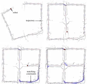
trajectory robot
constraints matching
Fig. 1. Four snapshots created while incrementally learning a map.
In this paper, we present an efficient online optimization algorithm which can be used to solve the so-called “graph-based” or “network-“graph-based” formulation of the SLAM prob-lem. Here, the poses of the robot are modeled by nodes in a graph and constraints between poses resulting from observations or from odometry are encoded in the edges between the nodes. Our method belongs to the same class of techniques of Olson’s algorithm or MLR [8]. It focuses on computing the best map and it assumes that the constraints are given. Techniques like the ATLAS framework [9] or hierarchical SLAM [10], for example, can be used to obtain the necessary data associations (constraints). They also apply a global optimization procedure to compute a consistent map. One can replace these optimization procedures by our algorithm and in this way make them more efficient.
Our approach combines the ideas of adaptive learning rates with a tree-based parameterization of the nodes when applying stochastic gradient descent. This yields an online algorithm that can efficiently compute network configura-tions with low errors. An application example is shown in Figure 1. It depicts four snapshots of our online approach during a process of building a map from the ACES dataset.
II. RELATEDWORK
A large number of mapping approaches has been presented in the past and a variety of different estimation techniques have been used to learn maps. One class of approaches uses constraint networks to represent the relations between poses and observations.
Lu and Milios [1] were the first who used constraint networks to address the SLAM problem. They proposed a brute force method that seeks to optimize the whole network at once. Gutmann and Konolige [11] presented an effective way for constructing such a network and for detecting loop closures while running an incremental estimation algorithm. Freseet al.[8] described a variant of Gauss-Seidel relaxation called multi-level relaxation (MLR). It applies relaxation at different resolutions.
Olson et al. [2] were the first who applied a variant of stochastic gradient descent to compute solutions to this family of problems. They propose a representation of the nodes which enables the algorithm to perform efficient updates. Our previously presented method [3] introduced the tree parameterization that is also used in this paper. Subsequently, Olsonet al.[6] presented an online variant of their method using adaptive learning rates. In this paper, we integrate such learning rates into the tree-based parameteri-zation which yields a solution to the online SLAM problem that outperforms the individual methods.
Kaessel al.[7] proposed an on-line version of the smooth-ing and mappsmooth-ing algorithm for maximum likelihood map estimation. This approach relies on a QR factorization of the information matrix and integrates the new measurements as they are available. Using the QR factorization, the poses of the nodes in the network can be efficiently retrieved by back substitution. Additionally they keep the matrices sparse via occasional variable reordering. Frese [12] proposed the Treemap algorithm which is able to perform efficient updates of the estimate by ignoring the weak correlations between distant locations.
The contribution of this paper is an efficient online ap-proach for learning maximum likelihood maps. It integrates adaptive learning rates into a tree-based network optimization technique using a variant of stochastic gradient descent. Our approach presents an efficient way of selecting only the part of the network which is affected by newly incorporated data. Furthermore, it allows to delay the optimization so that the network is only updated if needed.
III. STOCHASTICGRADIENTDESCENT FORMAXIMUM
LIKELIHOODMAPPING
Approaches to graph-based SLAM focus on estimating the most likely configuration of the nodes and are therefore referred to as maximum-likelihood (ML) techniques [8], [1], [2]. The approach presented in this paper also belongs to this class of methods.
The goal of graph-based ML mapping algorithms is to find the configuration of the nodes that maximizes the likelihood of the observations. Let x = (x1 · · · xn)T be a vector of
parameters which describes a configuration of the nodes. Let
δji and Ωji be respectively the mean and the information
matrix of an observation of node j seen from node i. Let
fji(x)be a function that computes a zero noise observation
according to the current configuration of the nodesj andi. Given a constraint between node j and node i, we can
define theerroreji introduced by the constraint as
eji(x) = fji(x)−δji (1)
as well as the residual rji = −eji(x). Let C =
{hj1, i1i, . . . ,hjM, iMi} be the set of pairs of indices for
which a constraintδjmim exists. The goal of a ML approach
is to find the configuration x∗ of the nodes that minimized the negative log likelihood of the observations. Assuming the constraints to be independent, this can be written as
x∗= argmin
x
X
hj,ii∈C
rji(x)TΩjirji(x). (2)
In the remainder of this section we describe how the general framework of stochastic gradient descent can be used for minimizing Eq. (2) and how to construct a parameterization of the network which increases the convergence speed.
A. Network Optimization using Stochastic Gradient Descent
Olson et al. [2] propose to use a variant of the pre-conditioned stochastic gradient descent (SGD) to address the compute the most likely configuration of the network’s nodes. The approach minimizes Eq. (2) by iteratively se-lecting a constraint hj, ii and by moving the nodes of the network in order to decrease the error introduced by the selected constraint. Compared to the standard formulation of gradient descent, the constraints are not optimized as a whole but individually. The nodes are updated according to the following equation:
xt+1 = xt+λ·H−1JjiTΩjirji (3)
Here x is the set of variables describing the locations of the poses in the network and H−1 is a preconditioning matrix. Jji is the Jacobian of fji, Ωji is the information
matrix capturing the uncertainty of the observation, rji is
the residual, andλis the learning rate which decreases with the iteration. For a detailed explanation of Eq. (3), we refer the reader to our previous works [3], [2].
In practice, the algorithm decomposes the overall problem into many smaller problems by optimizing subsets of nodes, one subset for each constraint. Whenever time a solution for one of these subproblems is found, the network is updated accordingly. Obviously, updating the different constraints one after each other can have antagonistic effects on the corre-sponding subsets of variables. To avoid infinitive oscillations, one uses the learning rate λ to reduce the fraction of the residual which is used for updating the variables. This makes the solutions of the different sub-problems to asymptotically converge towards an equilibrium point that is the solution reported by the algorithm.
B. Tree Parameterization
The poses p = {p1, . . . , pn} of the nodes define the
configuration of the network. The poses can be described by a vector of parametersx such that a bidirectional map-ping between pand x exists. The parameterization defines the subset of variables that are modified when updating a constraint. An efficient way of parameterizing the node is to
use a tree. One can construct a spanning tree (not necessarily a minimum one) from the graph of poses. Given such a tree, we define the parameterization for a node as
xi = pi−pparent(i), (4) wherepparent(i)refers to the parent of nodeiin the spanning tree. As defined in Eq. (4), the tree stores the differences between poses. This is similar in the spirit to the incremental representation used in the Olson’s original formulation, in that the difference in pose positions (in global coordinates) is used rather than pose-relative coordinates or rigid body transformations.
To obtain the difference between two arbitrary nodes based on the tree, one needs to traverse the tree from the first node upwards to the first common ancestor of both nodes and then downwards to the second node. The same holds for computing the error of a constraint. We refer to the nodes one needs to traverse on the tree as the path of a constraint. For example, Pji is the path from nodei to node j for the
constrainthj, ii. The path can be divided into an ascending partPji[−] of the path starting from nodei and a descending part Pji[+] to node j. We can then compute the residual in
the global frame by
r′ji = X k[−]∈P[−] ji xk[−]− X k[+]∈P[+] ji xk[+]+Riδji. (5)
HereRi is the homogeneous rotation matrix of the posepi.
It can be computed according to the structure of the tree as the product of the individual rotation matrices along the path to the root. Note that this tree does not replace the graph as an internal representation. The tree only defines the parameterization of the nodes.
Let Ω′
ji = RiΩjiRTi be the information matrix of a
constraint in the global frame. According to [2], we compute an approximation of the Jacobian as
Jji′ = X k[+]∈P[+] ji Ik[+]− X k[−]∈P[−] ji Ik[−], (6) withIk = (0 · · · 0 I |{z} kthelement
0 · · · 0). Then, the update of a constraint turns into
xt+1 = xt+λ|Pji|M−1Ω′jir
′
ji, (7)
where|Pji|refers to the number of nodes inPji. In Eq. (7),
we replaced the preconditioning matrixH−1with its scaled approximationM−1as described in [2]. This prevents from a computationally expensive matrix inversion.
Let thelevelof a node be the distance in the tree between the node itself and the root. We define the top node of a constraint as the node on the path with the smallest level. Our parameterization implies that updating a constraint will never change the configuration of a node with a level smaller than the level of the top node of the constraint.
In principle, one could apply the technique described in this section as a batch algorithm to an arbitrarily constructed spanning tree of the graph. However, our proposed method
uses a spanning tree which can be constructed incrementally, as described in the next section.
IV. ONLINENETWORKOPTIMIZATION
The algorithm presented in the previous section is a batch procedure. At every iteration, the poses of all nodes in the network are optimized. The fraction of the residual used in updating every constraint decreases over time with the learning rate λ, which evolves according to an harmonic progression. During online optimization, the network is dy-namically updated to incorporate new movements and obser-vations. In theory, one could also apply the batch version of our optimizer to correct the network. This, however, would require to compute a solution from scratch each time the robot moves or makes an observation which would obviously lead to an inefficient algorithm.
In this section we describe an incremental version of our optimization algorithm, which is suitable for solving on-line mapping problems. As pointed in [6] an incremental algorithm should have the following properties:
1) Every time a constraint is added to the network, only the part of the network which is affected by that constraint should be optimized. For example, when exploring new terrain, the effects of the optimization should not perturb distant parts of the graph.
2) When revisiting a known region of the environment it is common to re-localize the robot in the previously built map. One should use the information provided by the re-localization to compute a better initial guess for the position of the newly added nodes.
3) To have a consistent network, performing an opti-mization step after adding each constraint is often not needed. This happens when the newly added con-straints are adequately satisfied by the current network configuration. Having a criterion for deciding when to perform unnecessary optimizations can save a substan-tial amount of computation.
In the remainder of this section, we present four im-provements to the algorithm so that it satisfies the discussed properties.
A. Incremental Construction of the Tree
When constructing the parameterization tree online, we can assume that the input is a sequence of poses corre-sponding to a trajectory of the robot. In this case, subsequent poses are located closely together and there exist constraints between subsequent poses resulting from odometry or scan-matching. Further constraints between arbitrary nodes result from observations when revisiting a place in the environment. We proceed as follows: the oldest node is the root of the tree. When adding a node i to the network, we choose as its parent the oldest node for which a constraint to the node
iexists. Such a tree can be constructed incrementally since adding a new node does not require to change the existing parts of the tree.
The posepi and parameterxi of a newly added nodeiis
the connecting constraint as
pi = pparent(i)⊕δi,parent(i) (8)
xi = pi−pparent(i). (9) The parent node represents an already explored part of the environment and the constraint between the new node and the parent can be regarded as a localization event in an already constructed map, thus satisfying Property 2. As shown in the experiments described below, this initialization appears to be a good heuristic for determining the initial guess of the pose of a newly added node.
B. Constraint Selection
When adding a constraint hj, ii to the graph, a subset of nodes needs to be updated. This set depends on the topology of the network and can be determined by a variant of breadth first visit. LetGj,ibe the minimal subgraph that contains the
added constraint and has only one constraint to the rest of the graph. Then, the nodes that need to be updated are all nodes of the minimal subtree that containsGj,i. The precise
formulation on how to efficiently determine this set is given by Algorithm 1.
Data:hj, ii: the constraint,G: the graph,T: the tree. Result:Nji: the set of affected nodes,Eji: the affected
constraints.
Queuef= childrenOf(topNode(hj, ii));
Eji:= edgesToChildren(topNode(hj, ii)); foreachha, bi ∈ Ejido
ha, bi.mark=true;
end
whilef6={}do Noden:= first(f);
n.mark:=true
foreachha, bi ∈edgesOf(n)do
ifha, bi.mark=truethen
continue; end
Nodem:= (a=n)?b:a;
ifm= parent(n) orm.mark=truethen continue; end ha, bi.mark=true; Eji:=Eji∪ {ha, bi}; ifha, bi ∈ T then f:=f∪ {m}; else f:=f∪childrenOf(topNode(ha, bi)); end end f:= removeFirst(f); Nji:=Nji∪ {n}; end
Algorithm 1: Construction of the set of nodes affected by a constraint. For readability we assume that the frontier f can contain only the nodes which are not already marked.
Note that the number of nodes in Gj,i does depend only
on the root of the tree and on the overall graph. It contains all variables which are affected by adding the new costraint hi, ji.
C. Adaptive Learning Rates
Rather than using one learning rate λ for all nodes, the incremental version of the algorithm uses spatially adaptive learning rates introduced in [6]. The idea is to assign an individual learning rate to each node, allowing different parts of the network to be optimized at different rates. These learning rates are initialized when a new constraint is added to the network and they decrease with each iteration of the algorithm. In the following, we describe how to initialize and update the learning rates and how to adapt the update of the network specified in Eq. (7).
a) Initialization of the learning rates: When a new
constrainthj, iiis added to the network, we need to update the learning rates for the nodes Nji determined in the
previous section. First, we compute the learning rateλ′ji for
the newly introduced information. Then, we propagate this learning rate to the nodesNji.e
A proper learning rate is determined as follows. Let βji
be the fraction of the residual that would appropriately fuse the previous estimate and the new constraint. Similar to a Kalman filter,βji is determined as
βji= Ωji(Ωji+ Ωgraphji )
−1
, (10)
where Ωji is the information matrix of the new constraint,
andΩgraphji is an information matrix representing the uncer-tainty of the constraints in the network. Based on Eq. (10), we can compute the learning rateλ′ji of the new constraint
as λ′ji= maxrow 1 |Pji| (βji⊘MΩ′ji) . (11)
Here⊘represents the row by row division (see [6] for further details). The learning rate of the constraint is then propagated to all nodesk∈ Njias
λk ← max(λk, λ′ji), (12)
where λk is the learning rate of the node k. According
to Eq. (11) constraints with large residuals result in larger learning rate increases than constraints with small residuals.
b) Update of the network: When updating the network,
one has to consider the newly introduced learning rates. During an iteration, we decrease the individual learning rates of the nodes according to a generalized harmonic progression [13]:
λk ←
λk
1 +λk
(13) In this way, one guarantees the strong monotonicity of λk
and thus the convergence of the algorithm to an equilibrium point.
The learning rates of the nodes cannot be directly used for updating the poses since Eq. (7) requires a learning rate for each constraint and not for each node. When updating the network given the constrainthj, ii, we obtain an average learning rate˜λji from the nodes onPjias
˜ λji = 1 |Pji| X k∈Pji λk. (14)
Then, the constraint update turns into ∆xk = λ˜ji|Pji|M−1Ω′jir
′
ji. (15)
D. Scheduling the Network Optimization
When adding a set of constraintshj, ii ∈ Cnewto a network without performing an optimization, we can incrementally compute the error of the network as
enew=
X
hj,ii∈Cold
rTjiΩjirji+
X
hj,ii∈Cnew
rjiTΩjirji. (16)
Here enew is the new error and Cold refers to the set of constraints before the modification.
To avoid unnecessary computation, we perform the opti-mization only if needed. This is the case when the newly incorporated information introduced a significant error com-pared to the error of the network before. We perform an optimization step if
enew
|Cnew|+|Cold| > αhj,imaxi∈Cold
rjiTΩjirji. (17)
Here α is a user-defined factor that allows the designer of a mapping system to adapt the quality of the incremental solutions to the needs of the specific application.
If we assume that the network in Cold has already con-verged, this heuristic triggers an optimization only if a signif-icant inconsistency is revealed. Furthermore, the optimization only needs to be performed for a subset of the network and not for the whole network. The subset is given by
E = [
hj,ii∈Cnew
Eji. (18)
HereEji is the set of constraints to be updated given a new
constrainthj, ii ∈ Cnew. The setsEjiare computed according
to Algorithm 1. This criterion satisfies Property 3 and leads to an efficient algorithm for incrementally optimizing the network of constraints.
V. EXPERIMENTS
This section is designed to evaluate the effectiveness of the proposed methods to incrementally learn maximum likelihood maps. We first show that such a technique is well suited to generate accurate grid maps given laser range data and odometry from a real robot. Second, we provide simulation experiments to evaluate the evolution of the error and provide comparisons to our previously proposed tech-niques [3], [2], [6]. Finally, we illustrate the computational advantages resulting from our algorithm.
A. Real World Experiments
To illustrate that our technique can be used to learn maps from real robot data, we used the freely available ACES dataset. The motivating example shown in Figure 1 depicts four different maps computed online by our incremental mapping technique. During this experiment, we extracted constraints between consecutive poses by means of pairwise scan matching. Loop closures were determined by localizing
Fig. 2. Network used in the simulated experiments. Left: initial guess. Right: ground truth.
0.001 1 1000
0 5 10 15 20 25 30
error per constraint
iteration Olson Offline Olson Incremental Tree Offline Tree Incremental 0.001 1 1000 0 5 10 15 20 25 30
error per constraint
iteration
Olson Offline Olson Incremental Tree Offline Tree Incremental
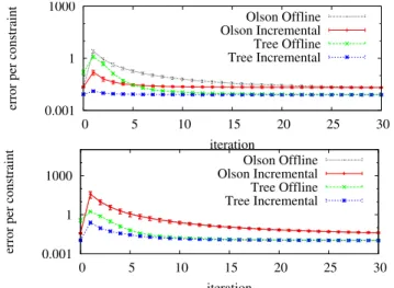
Fig. 3. Statistical experiments showing the evolution of the error per iteration of the algorithm. Top: situation in which the robot is closes a small loop. Bottom: closure of a large loop. The statistics have been generated by considering 10 different realizations of the observation noise along the same path.
the robot in the previously built map by means of a particle filter.
As can be seen, our approach leads to accurate maps for real robot data. Similar results were obtained with all datasets we found online or recorded on our own.
B. Statistical Experiments on the Evolution of the Error
In the these experiments, we moved a virtual robot on a grid world. An observation is generated each time the current position of the robot was close to a previously visited location. The observations are corrupted by a given amount of Gaussian noise. The network used in this experiment is depicted in Figure 2.
We compare our approach named Tree Incrementalwith its offline variant [3] called Tree Offline which solves the overall problem from scratch. In addition to that, we compare it to the offline version without the tree optimization [2] called Olson Offline as well as its incremental variant [6] referred to asOlson Incremental. For space reasons, we omit comparisons to LU decomposition, EKF, and Gauss-Seidel. The advantages of our method over these other methods is similar to those previously reported [2].
To allow a fair comparison, we disabled the scheduling of the optimization of Eq. (17) and we performed 30 iterations every time 16 constraints were added to the network. During the very first iterations, the error of all approaches may show
0 0.05 0.1 0.15 0.2 0.25 0.3 0 1000 2000 3000 4000 time Tree Offline Tree Incremental 0 0.01 0.02 0.03 0.04 0 1000 2000 3000 4000 error/constraint constraints Treemap Tree Incremental
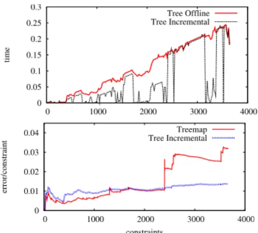
Fig. 4. Top: runtime comparison of the offline and the incremental approaches using a tree parameterization. The optimization is performed only when the error condition specified by Eq. (17) was verified. Bottom: Comparison of the evolution of the global error between Treemap[12] and the online version of our approach.
an increase, due to the bigger correction steps which result from increasing the learning rates.
Figure 3 depicts the evolution of the error for all four techniques during a mapping experiment. We depicted two situations. In the first one, the robot closed a small loop. As can be seen, the introduced error is small and thus our approach corrects the error within 2 iterations. Both incre-mental techniques perform better than their offline variants. The approach proposed in this paper outperforms the other techniques. The same holds for the second situation in which the robot was closing a large loop. Note that in most cases, one iteration of the incremental approach can be carried out faster, since only a subpart of the network needs to be updated.
C. Runtime Comparison
Finally, we evaluated our incremental version and its of-fline variant with respect to the execution time. Both methods where executed only when needed according to our criterion specified by Eq. (17). We measured the time needed to run the individual approach until convergence to the same low error configuration, or until a maximum number of iterations (30) was reached. As can be seen in Figure 4(top), the incremental technique requires significantly less operations and thus runtime to provide equivalent results in terms of error. Figure 4(bottom) shows the error plot of a comparison of our approach and Treemap [12] proposed by Frese. As shown in the error-plot, in the beginning Treemap performs slightly better than our algorithm, due to the exact calculation of the Jacobians. However, when closing large loops Treemap is more sensitive to angular wraparounds (see increase of the error at constraint 2400 in Figure 4). This issue is typically better handled by our iterative procedure. Overall, we observed that for datasets having a small noise Treemap provides slightly better estimates, while our approach is generally more robust to extreme conditions.
VI. CONCLUSION
In this paper, we presented an efficient online solution to the optimization of constraint networks. It can incrementally
learn maps while the robot moves through the environ-ment. Our approach optimizes a network of constraints that represents the spatial relations between the poses of the robot. It uses a tree-parameterization of the nodes and applies a variant of gradient descent to compute network configurations with low errors.
A per-node adaptive learning rate allows the robot to re-use already computed solutions from previous steps, to up-date only the parts of the network, which are affected by the newly incorporated information, and to start the optimization approach only if the new data causes inconsistencies with the already computed solution. We tested our approach on real robot data as well as with simulated datasets. We compared it to recently presented online and offline methods that also address the network-based SLAM problem. As we showed in practical experiments, our approach converges faster to a configuration with small errors.
ACKNOWLEDGMENT
The authors gratefully thank Udo Frese for providing us his Treemap implementation. This work has partly been supported by the DFG under contract number SFB/TR-8 (A3), by the EC under contract number FP6-IST-34120-muFly, and FP6-2005-IST-6-RAWSEEDS.
REFERENCES
[1] F. Lu and E. Milios, “Globally consistent range scan alignment for environment mapping,”Journal of Autonomous Robots, vol. 4, 1997. [2] E. Olson, J. Leonard, and S. Teller, “Fast iterative optimization of pose graphs with poor initial estimates,” inProc. of the IEEE Int. Conf. on Robotics & Automation (ICRA), 2006, pp. 2262–2269.
[3] G. Grisetti, C. Stachniss, S. Grzonka, and W. Burgard, “A tree parameterization for efficiently computing maximum likelihood maps using gradient descent,” in Proc. of Robotics: Science and Systems (RSS), Atlanta, GA, USA, 2007. [Online]. Available: http://www.informatik.uni-freiburg.de/ stachnis/pdf/grisetti07rss.pdf [4] R. Smith, M. Self, and P. Cheeseman, “Estimating uncertain spatial
realtionships in robotics,” inAutonomous Robot Vehicles, I. Cox and G. Wilfong, Eds. Springer Verlag, 1990, pp. 167–193.
[5] M. Montemerlo and S. Thrun, “Simultaneous localization and mapping with unknown data association using FastSLAM,” inProc. of the IEEE Int. Conf. on Robotics & Automation (ICRA), Taipei, Taiwan, 2003. [6] E. Olson, J. Leonard, and S. Teller, “Spatially-adaptive learning rates
for online incremental slam,” in Robotics: Science and Systems, Atlanta, GA, USA, 2007.
[7] M. Kaess, A. Ranganathan, and F. Dellaert, “iSAM: Fast incremental smoothing and mapping with efficient data association,” inProc. of the IEEE Int. Conf. on Robotics & Automation (ICRA), 2007. [8] U. Frese, P. Larsson, and T. Duckett, “A multilevel relaxation
algo-rithm for simultaneous localisation and mapping,”IEEE Transactions on Robotics, vol. 21, no. 2, pp. 1–12, 2005.
[9] M. Bosse, P. Newman, J. Leonard, and S. Teller, “An ALTAS framework for scalable mapping,” inProc. of the IEEE Int. Conf. on Robotics & Automation (ICRA), Taipei, Taiwan, 2003.
[10] C. Estrada, J. Neira, and J. Tard´os, “Hierachical slam: Real-time accurate mapping of large environments,” IEEE Transactions on Robotics, vol. 21, no. 4, pp. 588–596, 2005.
[11] J.-S. Gutmann and K. Konolige, “Incremental mapping of large cyclic environments,” inProc. of the IEEE Int. Symposium on Computational Intelligence in Robotics and Automation (CIRA), Monterey, CA, USA, 1999, pp. 318–325.
[12] U. Frese, “Treemap: Ano(logn)algorithm for indoor simultaneous localization and mapping,”Journal of Autonomous Robots, vol. 21, no. 2, pp. 103–122, 2006.
[13] H. Robbins and S. Monro, “A stochastic approximation method,” Annals of Mathematical Statistics, vol. 22, pp. 400–407, 1951.