Data Acquisition and View Planning for 3-D Modeling Tasks
Paul S. Blaer and Peter K. Allen
Abstract— In this paper we address the joint problems of automated data acquisition and view planning for large–scale indoor and outdoor sites. Our method proceeds in two distinct stages. In the initial stage, the system is given a 2-D map with which it plans a minimal set of sufficient covering views. We then use a 3-D laser scanner to take scans at each of these views. When this planning system is combined with our mobile robot, it automatically computes and executes a tour of these viewing locations and acquires the views with the robot’s onboard laser scanner. These initial scans serve as an approximate 3-D model of the site. The planning software then enters a second stage in which it updates this model by using a voxel-based occupancy procedure to plan the next best view. This next best view is acquired, and further next best views are sequentially computed and acquired until a complete 3-D model is obtained. Results are shown for Fort Jay on Governors Island in the City of New York and for the church of Saint Menoux in the Bourbonnais region of France.
I. INTRODUCTION
Dense and detailed 3-D models of large structures can be useful in many fields. These models can allow engineers to analyze the stability of a structure and then test possible corrections without endangering the original. The models can also provide documentation of historical sites in danger of destruction and archaeological sites at various stages of an excavation. With detailed models, professionals and students can tour such sites from thousands of miles away.
Modern laser range scanners will quickly generate a dense point cloud of measurements; however, many of the steps needed for 3-D model construction require time-consuming human involvement. These steps include the planning of the viewing locations as well as the acquisition of the data at multiple viewing locations. By automating these tasks, we will ultimately be able to speed this process significantly. A plan must be laid out to determine where to take each individual scan. This requires choosing efficient views that will cover the entire surface area of the structure without occlusions from other objects and without self occlusions from the target structure itself. This is the essence of the so– called view planning problem. Manually choosing the views can be time consuming in itself. Then the scanning sensor must be physically moved from location to location which is also time consuming and physically stressful.
Funded by NSF grants IIS-0121239 and ANI-00-99184.
Thanks to the National Park Service for granting us access to Governors Island and to the Governors Island staff: Linda Neal, Ed Lorenzini, Mike Shaver, Ilyse Goldman, and Dena Saslaw for their invaluable assistance.
Thanks to the scanning team of Hrvoje Benko, Matei Ciocarlie, Atanas Georgiev, Corey Goldfeder, Chase Hensel, Tie Hu, and Claire Lackner.
Both authors are with the Department of Computer Science, Columbia University, New York, NY 10027, USA
E-mail:{pblaer, allen}@cs.columbia.edu
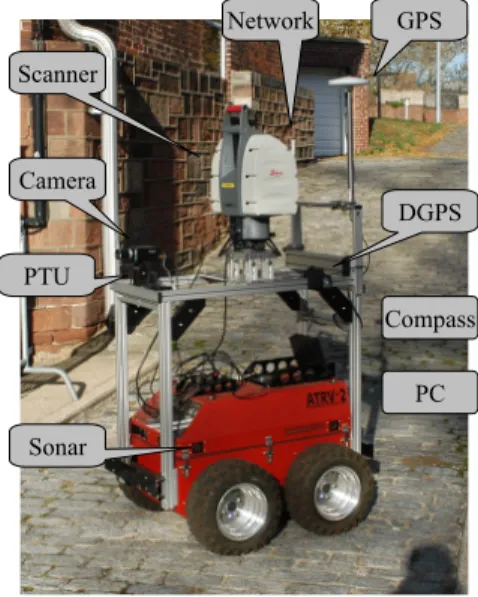
To assist with the planning for 3-D model construction, we have developed a two–stage view planning algorithm to decide automatically where to acquire scan data. We fur-ther automate the process by integrating this view planning system into our mobile robot platform, AVENUE [3] (see Fig. I). AVENUE is a laser–scanner–equipped robot capable of navigating itself through various environments. The view planning system is added to our previously developed local-ization ([10]) and low–level navigation software, allowing the robot to implement its plan and acquire a model of the location with minimal human assistance.
GPS DGPS PC Compass Sonar Network Scanner Camera PTU
Fig. 1. The ATRV-2 AVENUE Based Mobile Robot.
II. RELATED WORK
Currently there are a number of research projects focusing on three-dimensional models of urban scenes and outdoor structures. These projects include the 3-D city model con-struction project at Berkeley [9], the outdoor map building project at the University of Tsukuba [18], the MIT City Scan-ning Project [26], the volumetric robotic mapping project by Thrun et al. [27] and the UrbanScape project [2]. However, for the most part, these methods focus on data fusion issues and leave the planning to a human operator.
The view planning problem can be described as the task of finding a set of sensor configurations which efficiently and accurately fulfill a modeling or inspection task. Two major surveys of the topic exist including an earlier survey of computer vision sensor planning by Tarabanis et al [23]
and a more recent survey of view planning specifically for 3-D vision by Scott et al [21].
The model-based methods are the inspection methods in which the system is given some initial model of the scene. Early research focused on planning for 2-D camera-based systems. Included in this are works by Cowan and Kovesi [7] and by Tarabanis et al. [24]. Later, these methods were extended to the 3-D domain in works by Tarbox and Gottschlich [25]. We can also include the art gallery problems in this category. In two dimensions, these problems can be approached with traditional geometric solutions such as in Xie et al. [28] or with randomized methods such as in Gonz´alez-Ba˜nos et al. [11]. The art gallery approach has been applied to 3-D problems by Danner and Kavraki [8].
The non-model-based methods seek to generate models with no prior information. These include volumetric methods such as in Connolly [6], Massios and Fisher [15], and Low et al. [14]. There are also surface-based methods which include Maver and Bajcsy [16], Pito [19], Reed and Allen [20], and Sequeira et al ([22]). View planning for 2-D map construction with a mobile robot is addressed by Gonz´alez-Ba˜nos et al [12]. N¨uchter et al [17] address view planning for 3-D scenes with a mobile robot. Next best views are chosen by maximizing the amount of 2-D information (information on the ground plane only) that can be obtained at a chosen location; however, 3-D data are actually acquired.
III. THE TWO STAGE PLANNING ALGORITHM
A. Phase 1: Initial Model Construction
In the first stage of our modeling process, we wish to compute and acquire an initial model of the target region. This model will be based on limited information about the site and will likely have gaps which must be filled in during the second stage of the process. The data acquired in the initial stage will serve as a seed for the boostrapping method used to complete the model.
The procedure for planning the initial views makes use of a two-dimensional map of the region to plan a series of environment views for our scanning system to acquire. Maps such as these are commonly available for large scale sites. All scanning locations in this initial phase are planned in advance, before any data acquisition occurs.
Planning these locations resembles the art gallery problem, which asks where to optimally place guards such that all walls of the art gallery can be seen by the guards. We wish to find a set of positions for our scanner such that it can image all of the walls in our 2-D environment map. This view planning strategy makes the assumption that if we can see the 2-D footprint of a wall then we can see the wall in 3-D. In practice, this is rarely the case, because a 3-D part of a wall that is not visible in the 2-D map might obstruct another part of the scene. However, for an initial model of the scene to be used later for refinement, this assumption should give us sufficient coverage.
The traditional art gallery problem assumes that the guards have a 360 degree field of view, have an unlimited range,
and can view a wall at any grazing angle. None of these as-sumptions are true for most laser scanners, so the traditional methods do not apply to our problem. Gonz´alez-Ba˜nos et al [11] proposed a randomized method for approximating solutions to the art gallery problems. We have chosen to extend their randomized algorithm to include the visibility constraints of our sensor.
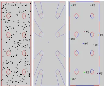
In our version of the randomized algorithm, a set of initial scanning locations are randomly distributed throughout the free space of the region to be imaged. The visibility polygon of each of these points is then computed based on the constraints of our sensor. Finally, an approximation for the optimal number of viewpoints needed to cover the boundaries of the free space is computed from this set of initial locations. For our initial test of this algorithm, we used a simulated environment. The region (see Fig. 2) represents a long hall-way with eight hexagonal pillars evenly spaced and located not far from the walls. In this test region, we chose to use a set of 200 random scanning locations (see the left side of Fig. 2). Next, the visibility of each viewpoint was computed. We used the ray-sweep algorithm [13] to compute the visibility polygon, and once the visibility polygons were computed we needed to clip their edges to satisfy our visibility constraints. An unclipped visibility polygon for one of the potential views can be seen in the center of figure 2. For the range constraints, we set a maximum and minimum range for the scanner. Any portion of an edge outside this range was discarded. We also constrained the grazing angle. Our sensor loses accuracy at grazing angles larger than 70o. Finally, our algorithm can constrain the field of view of the scanner. To make use of this constraint, we must also generate random headings together with each potential view location in the previous step of the algorithm. Our sensor has a 360o field of view, making this constraint unnecessary, but the algorithm does allow the method to be extended to other sensors. The clipped edges of the visibility polygon can be seen in blue on the right side of figure 2.
Finally, we utilized a greedy cover algorithm to select an approximation for the minimum number of viewpoints needed to cover the entire scene. In the simulated example, our algorithm returns between eight and ten scanning loca-tions (see Fig. 2) with 100% coverage of the region’s obstacle boundary. The 2-D planner is summarized in algorithm 1.
Algorithm 1The 2-D View Planning Algorithm. It must be given an initial 2-D mapM to plan the initial views.
1: procedure2DPLAN(M)
2: Randomly distribute candidate viewsV in the map
3: for allviewsvinV do
4: Compute the visibility polygonpofv 5: Clippto sensor range
6: Clippto maximum grazing angle
7: Clippto field of view
8: end for
9: Find a greedy cover,G, from the potential viewsV
10: returnG .the planned views
11: end procedure
Fig. 2. The initial simulated test region for the first phase of our view planning algorithm together with an initial set of 200 viewpoints randomly distributed throughout the free space of the region (left). The unclipped visibility polygon of one of the potential views (center). The final set of 10 scanning locations chosen for our simulated test region, with the clipped obstacle edges for scanning location #0 indicated in blue (right). All the figures in this paper should be viewed in color.
system must acquire and merge them. When the system is used to assist in manual scanning projects, the order in which the scans are taken does not matter. However, when used with our mobile robot, an efficient tour of the view locations is crucial. A typical scan can take 40 minutes to an hour. Traveling between sequential viewing locations typically takes less than that; however, if we zig-zag across the site rather than follow an optimized tour, travel time can begin to approach scan time and slow the algorithm.
This problem can be formulated as a traveling salesperson problem (TSP). Good approximation algorithms exist to compute a near optimal tour of the observation locations. The cost of traveling between two observation points can be computed by finding an efficient, collision free, path between the two points and using the length of that path as the cost. The robot’s Voronoi–diagram–based path planning module, described in [4], generates such paths between two locations on the 2D map of the environment, and we can use that method to compute edge costs for our TSP implementation. With the tour of the initial viewpoints computed, we can then allow the underlying navigation software to bring the robot to each scanning position and acquire the scans.
Registration of the scans into one merged model is re-quired. For our experiments, we used highly reflective targets placed in the scene to register one scan to the next. The 2-D algorithm can be modified to enforce an overlap constraint during the greedy cover of the potential scanning locations, allowing us to use automatic registration algorithms such as the iterative closest point algorithms.
B. Phase 2: 3-D View Planning
After the initial modeling phase has been completed, we have a preliminary model of the environment. The model
will have holes in it, many caused by originally undetectable occlusions. We now implement a 3-D view planner that makes use of this initial 3-D model to plan efficiently for further views. Instead of planning all of its views at once, the modeling phase takes the initial model and plans a single next best view that will gather what we estimate to be the most new information possible, given the known state of the world. This scan is acquired and the new data are integrated into the model of the world and the next best view is planned.
1) Voxel Space: To keep track of the parts of the scene that have not yet been imaged, we use a voxel representation of the data. Because this is a large scale imaging problem, the voxels can be made the large size of one meter cubed and still be sufficient to allow occlusion computation in our views. Although the planner uses the data at a reduced resolution, the full data are still used in constructing the final model.
The voxel representation is generated from the point cloud. Before the initial model is inserted, all voxels in the grid are labeled as unseen. For each scan from the initial model, voxels that contain at least one data point from that scan are marked as seen-occupied. A ray is then traced from each data point back to the scanner position. Each unseen voxel that it crosses is marked as seen-empty. If the ray passes through a voxel that was already labeled as seen-occupied, it means that the voxel itself has already been filled by a previous scan or another part of the current scan. These are typically partially occupied voxels and we allow the ray to pass through it without modifying its status as seen-occupied.
2) Next Best View: Our final modeling phase must now plan and acquire next best views sequentially. We are re-stricted to operating on the ground plane with our mobile robot. We can exploit the fact that we have a reasonable two-dimensional map of the region. This 2-D map gives us the footprints of the buildings as well as an estimate of the free space on the ground plane in which we can operate. We mark the voxels which intersect this ground plane within the free space defined by our 2-D map as being candidate views. We wish to choose a location on this ground plane grid that maximizes the number of unseen voxels that can be viewed from a single scan. Considering every unseen voxel in this procedure is unnecessarily expensive. We need to focus on those unseen voxels that are most likely to provide us with information about the facades of the buildings. These voxels are the ones that fall on the boundaries between seen-empty regions and unseen regions where we are most likely to see previously occluded structures viewable by the scanner. If an unseen voxel is surrounded by seen-occupied voxels or even by other unseen voxels, it may never be visible by any scan. We therefore choose to consider only unseen voxels that are adjacent to at least one seen-empty voxel. Such unseen voxels will be labeled as boundary unseen voxels.
At each candidate view, we keep a tally of the number of boundary unseen voxels that can be seen from that position. To do this, we trace a ray from the candidate view to the center of each boundary unseen voxel. If that ray intersects any seen-occupied or unseen voxels, we discard it because it will likely be occluded. If the ray’s length is outside the
scanner’s range, then we discard the ray as well. If a ray has not been discarded by either the occlusion or range condition, we can safely increment the tally of the candidate view from which the ray emanates. At the end of this calculation, the ground plane position with the highest tally is chosen as the next scan location. When using the mobile robot, it again computes the Voronoi-based path and navigates to the chosen position. It triggers a scan once it has arrived, and that scan is integrated into the point cloud model and the voxel representation. This second stage is repeated until we reach a sufficient level of coverage. To terminate the algorithm, we look at the number of boundary unseen voxels that would be resolved by the next iteration. If that number falls below some threshold value, the algorithm terminates; otherwise, it continues. The 3-D planner is summarized in algorithm 2.
Algorithm 2The 3-D View Planning Algorithm. It must be given an initial model of the worldC, a set of possible scanning locations
P, and a threshold value for unseen voxels as a stopping condition.
1: procedure3DPLAN(C,P,threshold)
2: Initialize voxel space fromC
3: for allunseen voxels,u, in the voxel spacedo 4: ifuhas a seen empty neighborthen
5: add utoU .the set of boundary unseen voxels
6: end if
7: end for 8: loop
9: for allpotential viewspinP do 10: Count members ofU that are visible
11: end for
12: ifmaxcount(p)< thresholdthen
13: break
14: end if
15: Acquire scan atpwith largest count
16: Merge new scan intoCand update voxel space
17: RecomputeU from the new voxel space
18: end loop
19: returnC .the updated model
20: end procedure
The algorithm is similar to a brute force computation. If the size of one dimension of the voxel grid is n, there could be O(n2) potential viewing locations. If there arem boundary unseen voxels, the cost of the algorithm could be as high asO(n2∗m). However, this cost is not prohibitive.mis small in comparison to the total number of voxels and many of then2 ground plane voxels are not potential view points because they fall within known obstacles. Furthermore, since most boundary unseen voxels only have one face exposed to the known world, the majority of the potential scanning locations can be quickly excluded.
IV. EXPERIMENTALRESULTS A. Phase 1 Applied Indoors and Outdoors
1) Saint Menoux: As part of a larger 3-D modeling effort, we have been involved in modeling the Romanesque churches of the Bourbonnais region of France [1]. We tested our 2-D planning algorithm in several of those churches, including the interior of the church of Saint Menoux. In this indoor experiment, we tested the algorithm itself by
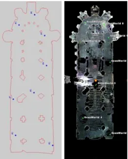
Fig. 3. On the left is the 2-D map of Saint Menoux’s interior. Also shown are the 8 scan locations determined by the initial two-dimensional view planner using a grazing angle constraint of 70o. On the right is a slice taken at floor level of the complete model acquired after taking all 8 scans.
moving our 360o field of view scanner manually to each of the planned views. We could not use the mobile robot indoors here because the robot makes extensive use of GPS in its navigation routines and GPS is typically not usable in an indoor environment. Also, the curch had a particularly cluttered environment containing numerous chairs and tables that left paths that were too narrow for our robot. However, as a sensor planning technique, our algorithms were very useful, even to human scanners.
For our test, we set the threshold such that the algorithm terminated if additional scans added less than 2% of the total boundaries of the target region. Our algorithm returned eight scanning locations for the test area (see the left of Fig. 3) giving us a coverage of 95% of the region’s obstacle boundary. In figure 3 we show a floor level slice of the resulting interior model of the church. In this experiment, as with all others, scans were merged using reflective targets scattered throughout the environment for registration.
2) Fort Jay: Fort Jay is a large fort located on Governors Island in the City of New York. With the kind permission of the National Park Service, we used this as our outdoor test bed for the system. We were given a floor plan of the fort which we divided into three distinct sections: the inner courtyard, the outer courtyard, and the moat.
We split the fort into these three sections because the transitions between them were not easily traversable by the robot. Also, because of sloped terrain, the robot could not operate in the outer courtyard or moat. As a result, these two outer regions were acquired by using our planning algorithm to make the decisions and then placing the scanner manually at the scanning locations. For the inner courtyard modeling, the mobile robot chose the scanning locations, planned the tour of those positions, and traversed the path, allowing us
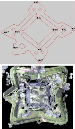
Fig. 4. On the top are the viewing locations chosen by the initial modeling phase for the outer courtyard of Fort Jay. On the bottom is the entire model of Fort Jay (seen from above) generated by the initial planning stage for the inner and outer courtyards and the moat.
to acquire the inner model with the mobile robot.
As with the previous experiment, we set our termination threshold to 2% of the total boundaries of the target region. Our algorithm produced seven locations in the inner court-yard, ten locations in the outer courtcourt-yard, and nine locations in the moat, giving us a coverage of 98% of the region’s obstacle boundary. In figure 4, one can see the planned locations for the outer courtyard as well as the entire initial model acquired by phase one of the algorithm.
B. Phase 2: Refinement of the Fort Jay Model
Fig. 5. A representation of the seen-occupied cells of Fort Jay’s voxel grid. It was constructed at the end of phase one from the point cloud acquired in section IV-A.2.
We now wish to refine the model of Fort Jay generated in the previous section, by using our 3-D planner. First, the initial model was inserted into the voxel space. On the
Fig. 6. On the left is a segment of the model of Fort Jay created during phase one of the algorithm. The hole in the left figure is caused by an unpredicted occlusion of one of the initial scanning locations. On the right is the same section of the model after the first two NBVs from phase two were computed and acquired.
ground level, the site was approximately 300x300 meters squared. No elevation measured was above 30 meters. Using a resolution of 1 meter cubed for our voxels, we had a grid of 2.7 million voxels. Of those voxels, most of them (2,359,321) were marked as empty, 68,168 were marked as seen-occupied (see Fig. 5), leaving 272,511 unseen voxels. Of those unseen voxels, only 25,071 were boundary unseen.
Next, we computed the potential viewing location that could see the most boundary unseen voxels. It turned out that this view was attempting to resolve part of a very large occlusion caused by the omission of a building on the 2-D map of Fort Jay. The footprint map that we were given did not have this building indicated, and we decided it would be a more realistic experiment not to modify the given map. One can see the resulting hole in the model on the left of figure 6. The first NBV only resolved a portion of the occlusion. Our algorithm says that if a voxel is unseen, we have to assume that it could be occupied. As a result, we cannot plan an NBV that is located inside a region of unseen voxels. We can only aim at the frontier between the known and the unknown from a vantage point located in a seen-empty region. The next NBV that was computed resolved the entire occlusion (see the right of Fig. 6), since enough of the unseen region had been revealed as empty so as to safely place the scanner in a position that could see the entire occlusion.
For this experiment, we chose a threshold of 100 boundary unseen voxels as the cutoff for our algorithm. When it was estimated that the next best view would net fewer than this threshold number of voxels, the algorithm ter-minated. Ultimately we needed to compute five NBV’s in the outer courtyard, one NBV in the inner courtyard, and two additional NBV’s in the moat. Figure 7 summarizes the number of labeled voxels at each iteration of the algorithm as well as the runtime for each iteration. A typical runtime in our experiments was on the order of 15 to 20 minutes. Nevertheless, since a scan could take up to an hour to complete, the cost of this algorithm was acceptable. A view of the final model of Fort Jay can be seen in figure 8.
V. DISCUSSION AND CONCLUSIONS We presented a method for automated view planning in the construction of 3-D models of large indoor and outdoor scenes. We also integrated this algorithm into our mobile
At the Seen Boundary Visible Runtime end of: Occupied Unseen to NBV (minutes) 2-D Plan 68,168 25,071 1,532 21.25 NBV 1 70,512 21,321 1,071 19.30 NBV 2 71,102 18,357 953 18.93 NBV 3 72,243 17,156 948 18.72 NBV 4 73,547 15,823 812 16.59 NBV 5 74,451 14,735 761 16.43 NBV 6 75,269 13,981 421 15.82 NBV 7 75,821 13,519 255 15.60 NBV 8 76,138 13,229 98 15.22
Fig. 7. A summary of the number of labeled voxels after each iteration of the 3-D planning algorithm. The next to last column indicates the number of boundary unseen voxels that are actually visible to the next best view.
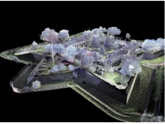
Fig. 8. A view of the final model of Fort Jay after all 34 scans from phases one and two were acquired.
robot, allowing us to acquire those views automatically. The procedure started from a 2-D map of the environment, which defined the robot’s free space. The method then progressed through (1) an initial stage in which a 3-D model was constructed by having the robot compute and acquire a set of initial scans using our 2-D view planning algorithm followed by (2) a dynamic refinement stage which made use of a voxel representation of the environment to successively plan next best views to acquire a complete model.
One could argue that requiring a 2-D map for exploration is too restrictive. For our work, however, the scenes in which we have the most interest, historical and urban sites, a 2-D map already exists. Nevertheless, we have explored sites using only the algorithm’s second stage [5], without an initial map. In our current work, by using the 2-D planner first, we reveal most of the scenes in advance, greatly decreasing the number of voxels that the 3-D algorithm must examine.
There are many paradigms for mobile robot exploration and mapping of environments. Our particular interest is in the construction of dense and detailed models of these environments, not in fast low resolution scans taken as a vehicle moves. Our scanning equipment is designed to maximize detail, and this causes scan times to be very long. With scan times of the order of an hour, the naive approach of taking essentially random scans as one navigates through the environment is unworkable. The view planning algorithms presented in this paper eliminate unnecessary scans and can reduce the time needed for detailed model building.
REFERENCES [1] http://www.learn.columbia.edu/bourbonnais/.
[2] A. Akbarzadeh, J.-M. Frahm, P. Mordohai, B. Clipp, C. Engels, D. Gallup, P. Merrell, M. Phelps, S. Sinha, B. Talton, L. Wang, Q. Yang, H. Stewenius, R. Yang, G. Welch, H. Towles, D. Nister, and M. Pollefeys. Towards urban 3d reconstruction from video. In
3DPVT, 2006.
[3] P. K. Allen, I. Stamos, A. Gueorguiev, E. Gold, and P. Blaer. Avenue: Automated site modeling in urban environments. In3DIM, 2001. [4] P. Blaer and P. K. Allen. Topbot: automated network topology
detection with a mobile robot. InIEEE ICRA, 2003.
[5] P. S. Blaer and P. K. Allen. View planning for automated site modeling. InIEEE ICRA, 2006.
[6] C. I. Connolly. The determination of next best views. InIEEE ICRA, 1985.
[7] C. K. Cowan and P. D. Kovesi. Automatic sensor placement from vision task requirements. IEEE PAMI, 10(3), May 1988.
[8] T. Danner and L. E. Kavraki. Randomized planning for short inspection paths. InIEEE ICRA, 2000.
[9] C. Frueh and A. Zakhor. Constructing 3d city models by merging ground-based and airborne views. InIEEE CVPR, 2003.
[10] A. Georgiev and P. K. Allen. Localization methods for a mobile robot in urban environments.IEEE Trans. on Robotics, 20(5), October 2004. [11] H. Gonz´alez-Banos and J. C. Latombe. A randomized art-gallery algorithm for sensor placement. InProc. of the 17th annual symposium on Computational Geometry, 2001.
[12] H. Gonz´alez-Banos, E. Mao, J. C. Latombe, T. M. Murali, and A. Efrat. Planning robot motion strategies for efficient model con-struction. InISRR, 1999.
[13] J. E. Goodman and J. O’Rourke.Handbook of discrete and computa-tional geometry. CRC Press, Inc., 1997.
[14] K.-L. Low and A. Lastra. Efficient constraint evaluation algorithms for hierarchical next-best-view planning. In3DVPT, 2006.
[15] N. A. Massios and R. B. Fisher. A best next view selection algorithm incorporating a quality criterion. InBritish Machine Vis. Conf., 1998. [16] J. Maver and R. Bajcsy. Occlusions as a guide for planning the next
view. IEEE PAMI, 15(5), May 1993.
[17] A. N¨uchter, H. Surmann, and J. Hertzberg. Planning robot motion for 3d digitalization of indoor environments. InICAR, 2003.
[18] K. Ohno, T. Tsubouchi, and S. Yuta. Outdoor map building based on odometry and rtk-gps position fusion. InIEEE ICRA, 2004. [19] R. Pito. A solution to the next best view problem for automated surface
acquisition. IEEE PAMI, 21(10), October 1999.
[20] M. K. Reed and P. K. Allen. Constraint-based sensor planning for scene modeling. IEEE PAMI, 22(12), December 2000.
[21] W. R. Scott, G. Roth, and J.-F. Rivest. View planning for automated three-dimensional object reconstruction and inspection. ACM Com-puting Surveys, 35(1), 2003.
[22] V. Sequeira and J. Gonc¸alves. 3d reality modelling: Photo-realistic 3d models of real world scenes. In3DPVT, 2002.
[23] K. A. Tarabanis, P. K. Allen, and R. Y. Tsai. A survey of sensor plan-ning in computer vision. IEEE Trans. on Robotics and Automation, 11(1):86–104, February 1995.
[24] K. A. Tarabanis, R. Y. Tsai, and P. K. Allen. The mvp sensor planning system for robotic vision tasks. IEEE Trans. on Robotics and Automation, 11(1), February 1995.
[25] G. H. Tarbox and S. N. Gottschlich. Planning for complete sensor coverage in inspection. Computer Vision and Image Understanding, 61(1), January 1995.
[26] S. Teller. Automatic acquisition of hierarchical, textured 3d geometric models of urban environments: Project plan. In Proc. of the Image Understanding Workshop, 1997.
[27] S. Thrun, D. H¨ahnel, D. Ferguson, M. Montemerlo, R. Triebel, W. Burgard, C. Baker, Z. Omohundro, S. Thayer, and W. Whittaker. A system for volumetric robotic mapping of abandoned mines. InIEEE ICRA, 2003.
[28] S. Xie, T. W. Calvert, and B. K. Bhatacharya. Planning views for the incremental construction of body models. InICPR, 1986.