Model Based Vehicle Tracking in Urban Environments

Model Based Vehicle Tracking in Urban Environments

Anna Petrovskaya and Sebastian Thrun

Stanford University Stanford, California 94305, USA

{ anya, thrun}@cs.stanford.edu

Abstract— Situational awareness is crucial for autonomous driving in urban environments. We present the moving vehicle tracking module we developed for our autonomous driving robot Junior. The robot won second place in the Urban Grand Challenge, an autonomous driving race organized by the U.S. Government in 2007. The module provides reliable detection and tracking of moving vehicles from a high-speed moving platform using laser range finders. Our approach models both dynamic and geometric properties of the tracked vehicles and estimates them using a single Bayes filter per vehicle. We show how to build consistent and efficient 2D representations out of 3D range data and how to detect poorly visible black vehicles. Experimental validation includes the most challenging conditions presented at the Urban Grand Challenge as well as other urban settings.

I. INTRODUCTION

Autonomously driving cars have been a long-lasting dream of robotics researchers and enthusiasts. Self-driving cars promise to bring a number of benefits to society, including prevention of road accidents, optimal fuel usage, comfort and convenience. In recent years the Defense Advanced Research Projects Agency (DARPA) has taken a lead on encouraging research in this area and organized a series of competitions for autonomous vehicles. In 2005 autonomous vehicles were able to complete a 131 mile course in the desert [1]. In the 2007 competition, the Urban Grand Challenge, the robots were presented with an even more difficult task: autonomous safe navigation in urban environments. In this competition the robots had to drive safely with respect to other robots, human-driven vehicles and the environment. They also had to obey the rules of the road as described in the California rulebook (see [2] for a detailed description of the rules). One of the most significant changes from the previous competition is the need for situational awareness of both static and dynamic parts of the environment. Our robot, Junior, won the second prize in the 2007 competition. An overview of Junior’s software and hardware architecture is given in [3]. In this paper we describe the approach we developed for detection and tracking of moving vehicles.

Vehicle tracking has been studied for several decades. A number of approaches focused on the use of vision exclusively [4], [5], [6]. Whereas others utilized laser range finders [7], [8], [9] sometimes in combination with vision [10]. We give an overview of prior art in Sect. II.

For our application we are concerned with laser based vehicle tracking from the autonomous robotic platform Ju-nior, to which we will also refer as the ego-vehicle (see Fig. 1). In contrast to prior art, we propose a model based approach which encompasses both geometric and dynamic

This work was in part supported by the Defense Advanced Research Projects Agency under contract number HR0011-06-C-0145. The opinions expressed in the paper are ours and not endorsed by the U.S. Government.

(a)

(b)

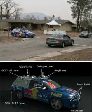
Fig. 1. (a) Our robot Junior (blue) negotiates an intersection with human-driven vehicles at the qualification event for the Urban Grand Challenge in November 2007. (b) Junior, is equipped with five different laser measurement systems, a multi-radar assembly, and a multi-signal inertial navigation system.

(a) without geometric model (b) with geometric model Fig. 2. Scans from vehicles are often split up into separate clusters by occlusion. Geometric vehicle model helps interpret the data properly. Purple rectangles group together points that have been associated together. In (b) the purple rectangle also denotes the geometric vehicle model. Gray areas are objects. Gray dotted lines represent laser rays. Black dots denote laser data points. (Best viewed in color.)

(a) without shape estimation (b) with shape estimation

Fig. 3. Vehicles come in different sizes. Accurate estimation of geometric shape helps obtain a more precise estimate of the vehicle dynamics. Solid arrows show the actual distance the vehicle moved. Dashed arrows show the estimated motion. Purple rectangles denote the geometric vehicle models. Black dots denote laser data points. (Best viewed in color.)

properties of the tracked vehicle in a single Bayes filter. The approach eliminates the need for separate data segmentation and association steps. We show how to properly model the dependence between geometric and dynamic vehicle properties using anchor point coordinates. The geometric model allows us to naturally handle the disjoint point clusters that often result from partial occlusion of vehicles (see Fig. 2). Moreover, the estimation of geometric shape leads to accurate prediction of dynamic parameters (see Fig. 3).

Further, we introduce an abstract sensor representation, we call the virtual scan, which allows for efficient computation and can be used for a wide variety of laser sensors. We present techniques for building consistent virtual scans from 3D range data and show how to detect poorly visible black vehicles in laser scans. Our approach runs in real time with an average update rate of 40Hz, which is 4 times faster than the common sensor frame rate of 10Hz. The results show that our approach is reliable and efficient even in challenging traffic situations presented at the Urban Grand Challenge.

II. BACKGROUND

Typically vehicle tracking approaches (e.g. [7], [8], [9], [10]) proceed in three stages: data segmentation, data associ-ation, and Bayesian filter update. During data segmentation the sensor data is divided into meaningful pieces (usually lines or clusters). During data association these pieces are assigned to tracked vehicles. Next a Bayesian filter update is performed to fit targets to the data.

The second stage - data association - is generally con-sidered the most challenging stage of the vehicle detection and tracking problem because of the association ambiguities that arise. Typically this stage is carried out using variants of multiple hypothesis tracking (MHT) algorithm (e.g. [8], [9]). The filter update is usually carried out using variants of Kalman filter (KF), which is augmented by interacting multiple model method in some cases [7], [9].

Although vehicle tracking literature primarily relies on variants of KF, there is a great body of multiple target tracking literature for other applications (see [11] for a summary) where parametric, sample-based, and hybrid filters are used. For example [12] uses a Rao-Blackwellized particle filter (RBPF) for multiple target tracking on simulated data. A popular alternative to MHT for data association is the joint probabilistic data association (JPDA) method. For example in [13] a JPDA particle filter is used to track multiple targets from an indoor mobile robot platform.

The work included in this paper has been presented at two conferences: [14] and [15]. In contrast to prior vehi-cle tracking literature, we utilize a model based approach, which uses RBPFs and eliminates the need for separate data

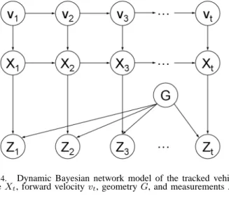
Fig. 4. Dynamic Bayesian network model of the tracked vehicle poseXt, forward velocityvt, geometryG, and measurementsZt.

segmentation and association stages. Our approach estimates position, velocity and shape of tracked vehicles.

III. REPRESENTATION

Our ego-vehicle is outfitted with the Applanix navigation system that provides pose localization with 1m accuracy. We further improved the localization module performance by observing lane markings [3]. Although global localization shifts may still occur, vehicle tracking is much more affected by localization drift rather than global shifts. For this reason we implemented smooth coordinates, which provide a locally consistent estimate of the ego-vehicle motion based on the data from the inertial measurement unit (IMU). As a result there is virtually no drift in the smooth coordinate system. Thus for the remainder of the paper we will assume that a reasonably precise pose of the ego-vehicle is always available.

Following the common practice in vehicle tracking, we will represent each vehicle with a separate Bayesian filter, and represent dependencies between vehicles via a set of local spatial constraints. Specifically we will assume that no two vehicles overlap, that all vehicles are spatially separated by some free space, and that all vehicles of interest are located on or near the road.

A. Probabilistic Model and Notation

For each vehicle we estimate its 2D position and orien-tation Xt = (xt, yt, θt) at time t, its forward velocity vt

and its geometry G (further defined in Sect. III-B). Also at each time step we obtain a new measurement Zt. See

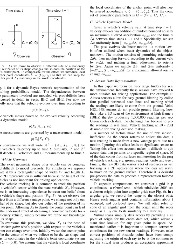
Fig. 5. As we move to observe a different side of a stationary car, our belief of its shape changes and so does the position of the car’s center point. To compensate for the effect, we introduce local anchor point coordinates C = (Cx, Cy) so that we can keep the anchor pointXt stationary in the world coordinates.

Fig. 4 for a dynamic Bayes network representation of the resulting probabilistic model. The dependencies between the parameters involved are modeled via probabilistic laws discussed in detail in Sects. III-C and III-E. For now we briefly note that the velocity evolves over time according to

p(vt|vt−1).

The vehicle moves based on the evolved velocity according to a dynamics model:

p(Xt|Xt₋₁, vt).

The measurements are governed by a measurement model:

p(Zt|Xt, G).

For convenience we will write Xt _{= (X}

1, X2, ..., Xt) for

the vehicle’s trajectory up to time t. Similarly, vt _{and Z}t

will denote all velocities and all measurements up to timet.

B. Vehicle Geometry

The exact geometric shape of a vehicle can be complex and difficult to model precisely. For simplicity we approx-imate it by a rectangular shape of width W and length L. The 2D representation is sufficient because the height of the vehicles is not important for driving applications.

For vehicle tracking it is common to track the position of a vehicle’s center within the state variableXt. However,

there is an interesting dependence between our belief about the vehicle’s shape and position (Fig. 5). As we observe the object from a different vantage point, we change not only our belief of its shape, but also our belief of the position of its center point. AllowingXtto denote the center point can lead

to the undesired effect of obtaining a non-zero velocity for a stationary vehicle, simply because we refine our knowledge of its shape.

To overcome this problem, we view Xt as the pose of

an anchor point who’s position with respect to the vehicle’s center can change over time. Initially we set the anchor point to be the center of what we believe to be the car shape and thus its coordinates in the vehicle’s local coordinate system areC= (0,0). We assume that the vehicle’s local coordinate system is tied to its center with the x-axis pointing directly forward. As we revise our knowledge of the vehicle’s shape,

the local coordinates of the anchor point will also need to be revised accordingly toC= (Cx, Cy). Thus the complete

set of geometric parameters isG= (W, L, Cx, Cy).

C. Vehicle Dynamics Model

Given a vehicle’s velocity vt−1 at time step t−1, the velocity evolves via addition of random bounded noise based on maximum allowed accelerationamax and the time delay ∆t between time stepst−1 andt. Specifically, we sample ∆v uniformly from [−amax∆t, amax∆t].

The pose evolves via linear motion - a motion law that is often utilized when exact dynamics of the object are unknown. The motion consists of perturbing orientation by ∆θ₁, then moving forward according to the current velocity by vt∆t, and making a final adjustment to orientation

by ∆θ₂. Again we sample ∆θ₁ and ∆θ₂ uniformly from [−dθmax∆t, dθmax∆t]for a maximum allowed orientation

changedθmax.

D. Sensor Data Representation

In this paper we focus on laser range finders for sensing the environment. Recently these sensors have evolved to be more suitable for driving applications. For example IBEO Alasca sensors allow for easy ground filtering by collecting four parallel horizontal scan lines and marking which of the readings are likely to come from the ground. Velodyne HDL-64E sensors do not provide ground filtering, however they take a 3D scan of the environment at high frame rates (10Hz) thereby producing 1,000,000 readings per second. Given such rich data, the challenge has become to process the readings in real time. Vehicle tracking at 10 - 20Hz is desirable for driving decision making.

A number of factors make the use of raw sensor data inefficient. As the sensor rotates to collect the data, each new reading is made from a new vantage point due to ego-motion. Ignoring this effect leads to significant sensor noise. Taking this effect into account makes it difficult to quickly access data that pertains to a specific region of space. Much of the data comes from surfaces uninteresting for the purpose of vehicle tracking, e.g. ground readings, curbs and tree tops. Finally, the raw 3D data wastes a lot of resources as vehicle tracking is a 2D application where the cars are restricted to move on the ground surface. Therefore it is desirable to pre-process the data to produce a representation tailored for vehicle tracking.

To expedite computations, we construct a grid in polar coordinates - a virtual scan - which subdivides360◦ _around

a chosen origin point into angular grids (see Fig. 6). In each angular grid we record the range to the closest obstacle. Hence each angular grid contains information about free, occupied, and occluded space. We will often refer to the cone of an angular grid from the origin until the recorded range as a ray due to its similarity to a laser ray.

Virtual scans simplify data access by providing a single point of origin for the entire data set, which allows con-stant time look-up for any given point in space. As we mentioned earlier it is important to compute correct world coordinates for the raw sensor readings. However, once the correct positions of obstacle points have been computed, adjusting the origin of each ray to be at the common origin for the virtual scan produces an acceptable approximation. Constructed in this manner, a virtual scan provides a compact representation of the space around the ego-vehicle classified

(a) anatomy of a virtual scan

(b) a virtual scan constructed from Velodyne data

Fig. 6. In (b) yellow line segments represent virtual rays. Colored points show the results of a scan differencing operation. Red points are new obstacles, green points are obstacles that disappeared, and white points are obstacles that remained unchanged or appeared in previously occluded areas. (Best viewed in color.)

into free, occupied and occluded. The classification helps us properly reason about what parts of an object should be visible as we describe in Sect. III-E.

For the purpose of vehicle tracking it is crucial to deter-mine what changes take place in the environment over time. With virtual scans these changes can be easily computed in spite of the fact that ego-motion can cause two consecutive virtual scans to have different origins. The changes are com-puted by checking which obstacles in the old scan are cleared by rays in the new scan and vice versa. This computation takes time linear in the size of the virtual scan and only needs to be carried out once per frame. Fig. 6(b) shows results of a virtual scan differencing operation with red points denoting new obstacles, green points denoting obstacles that disappeared, and white points denoting obstacles that remained in place or appeared in previously occluded areas. Virtual scans are a suitable representation for a wide variety of laser range finders. While this representation is easy to build for 2D sensors such as IBEO, for 3D range sensors additional considerations are required to produce consistent 2D representations. We describe these techniques in Sect. V.

E. Measurement Model

Given a vehicle’s poseX, geometry Gand a virtual scan

Z we compute the measurement likelihood p(Z|G, X) as follows. We position a rectangular shape representing the vehicle according to X andG. Then we build a bounding

(a)

(b)

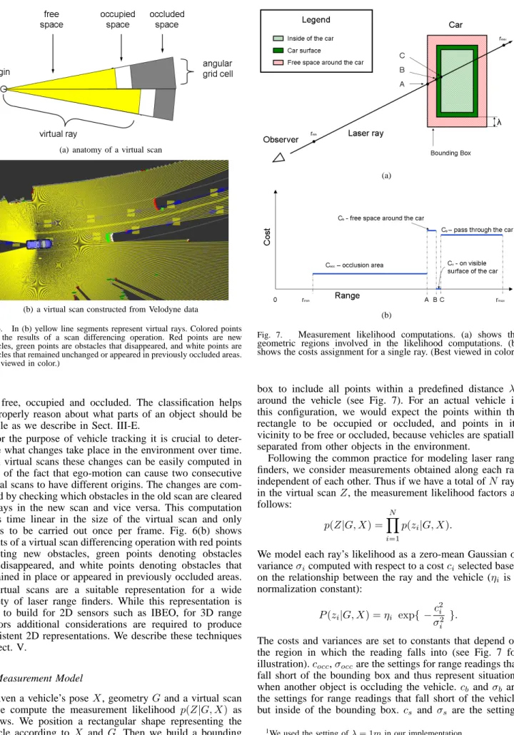
Fig. 7. Measurement likelihood computations. (a) shows the geometric regions involved in the likelihood computations. (b) shows the costs assignment for a single ray. (Best viewed in color.)

box to include all points within a predefined distance λ1

around the vehicle (see Fig. 7). For an actual vehicle in this configuration, we would expect the points within the rectangle to be occupied or occluded, and points in its vicinity to be free or occluded, because vehicles are spatially separated from other objects in the environment.

Following the common practice for modeling laser range finders, we consider measurements obtained along each ray independent of each other. Thus if we have a total ofN rays in the virtual scanZ, the measurement likelihood factors as follows: p(Z|G, X) = N Y i₌₁ p(zi|G, X).

We model each ray’s likelihood as a zero-mean Gaussian of varianceσicomputed with respect to a costciselected based

on the relationship between the ray and the vehicle (ηi is a

normalization constant): P(zi|G, X) =ηi exp{ − c2 i σ2 i }.

The costs and variances are set to constants that depend on the region in which the reading falls into (see Fig. 7 for illustration).cocc,σoccare the settings for range readings that

fall short of the bounding box and thus represent situations when another object is occluding the vehicle.cb andσb are

the settings for range readings that fall short of the vehicle but inside of the bounding box. cs andσs are the settings

for readings on the vehicle’s visible surface (that we assume to be of non-zero depth).cp,σpare used for rays that extend

beyond the vehicle’s surface.

The domain for each range reading is between minimum range rmin and maximum rangermax of the sensor. Since

the costs we select are piece-wise constant, it is easy to integrate the unnormalized likelihoods to obtain the nor-malization constants ηi. Note that for the rays that do not

target the vehicle or the bounding box, the above logic automatically yields uniform distributions as these rays never hit the bounding box.

Note that the proposed measurement model naturally handles partially occluded objects including objects that are “split up” by occlusion into several point clusters (see Fig. 2). In contrast these cases are often challenging for approaches that utilize separate data segmentation and correspondence methods.

IV. VEHICLETRACKING

Most vehicle tracking methods described in the literature apply separate methods for data segmentation and corre-spondence matching before fitting model parameters via extended Kalman filter (EKF). In contrast we use a single Bayesian filter to fit model parameters from the start. This is possible because our model includes both geometric and dynamic parameters of the vehicles and because we rely on efficient methods for parameter fitting. We chose the particle filter method for Bayesian estimation because it is more suitable for multi-modal distributions than EKF. Unlike the multiple hypothesis tracking (MHT) method commonly used in the literature, the computational complexity for our method grows linearly with the number of vehicles in the environment, because vehicle dynamics dictates that vehicles can only be matched to data points in their immediate vicinity. The downside of course is that in our case two targets can in principle merge into one. In practice we have found that it happens rarely and only in situations where one of the targets is lost due to complete occlusion. In these situations target merging is acceptable for our application.

We have a total of eight parameters to estimate for each vehicle: X = (x, y, θ), v, G = (W, L, Cx, Cy).

Computa-tional complexity grows exponentially with the number of parameters for particle filters. Thus to keep computational complexity low, we turn to RBPFs first introduced in [16]. We estimate X and v by samples and keep Gaussian es-timates for G within each particle. Below we give a brief derivation of the required update equations.

A. Update Equations

At each time steptwe produce an estimate of a Bayesian belief about the tracked vehicle’s trajectory, velocity and geometry based on a set of measurements:

Belt=p(Xt, vt, G|Zt).

We split up the belief into two conditional factors:

Belt=p(Xt, vt|Zt) p(G|Xt, vt, Zt).

The first factor encodes the vehicle’s motion posterior:

Rt=p(Xt, vt|Zt).

The second factor encodes the vehicle’s geometry posterior, conditioned on its motion:

St=p(G|Xt, vt, Zt).

Fig. 8. We determine ground readings by comparing angles between consecutive readings. If A, B, C are ground readings, then α is close to0and thuscosαis close to1.

The factor Rt is approximated using a set of particles; the

factorStis approximated using a Gaussian distribution (one

Gaussian per particle).

Detailed derivations of the update equations are provided in [15]. Here we briefly note that the motion update of the particle filter is carried out using the vehicle dynamics model described in Sect. III-C. The measurement update is carried out by computing the importance weightswtfor all particles:

wt=IESt₋₁[p(Zt|G, Xt) ].

In words, the importance weights are the expected value (with respect to the vehicle geometry prior) of the mea-surement likelihood. Using Gaussian approximations of the geometry prior St₋₁ and the measurement likelihood

p(Zt|G, Xt), this expectation can be computed in closed

form. We obtain a Gaussian approximation of the geometry prior recursively and apply Laplace’s method to approximate the measurement likelihood by a Gaussian.

B. Initializing and Discontinuing Tracks

New tracks are initialized in areas where scan differencing detects a change in data, that is not already explained by existing tracks. New tracks are fitted using the same measurement and motion models (Sects. III-E and III-C) that we use for vehicle tracking. The candidates are vetted for three frames before they can become “real tracks”. Detection of new vehicles is the most computationally expensive part of vehicle tracking. In order to achieve reliable vehicle detection in real time, we developed a number of optimization tech-niques. Details of the detection algorithm and optimizations can be found in [14].

We discontinue tracks if the target vehicle gets out of sensor range or moves too far away from the road2_{. We also}

discontinue tracks if the unnormalized weights have been low for several turns. Low unnormalized weights signal that the sensor data is insufficient to track the target, or that our estimate is too far away from the actual vehicle. This logic keeps the resource cost of tracking occluded objects low, yet it still allows for a tracked vehicle to survive bad data or complete occlusion for several turns. Since new track acquisition only takes three frames, it does not make sense to continue tracking objects that are occluded for significantly longer periods of time.

V. WORKING WITH3D RANGEDATA

As we explained in Sect. III-D, vehicle tracking is a 2D problem, for which compact 2D virtual scans are sufficient. However for 3D sensors, such as Velodyne, it is non-trivial to build consistent 2D virtual scans. These sensors provide immense 3D data sets of the surroundings, making 2_{A digital street map was available for our application in the Road} Network Definition Format (RNDF).

computational efficiency a high priority when processing the data. In our experience, the hard work pays off and the resulting virtual scans carry more information than 2D sensor data.

A. Classification of 3D Points

To produce consistent 2D virtual scans, we need to un-derstand which of the 3D data points should be considered obstacles. From the perspective of driving applications we are interested in the slice of space directly above the ground and about 2m high, as this is the space that a vehicle would actually have to drive through. Objects elevated more than 2m above ground - e.g. tree tops or overpasses - are not obstacles. The ground itself is not an obstacle (assuming the terrain is drivable). Moreover, for tracking applications low obstacles such as curbs should be excluded from virtual scans, because otherwise they can prevent us from seeing more important obstacles beyond them. The remaining ob-jects in the 2m slice of space are obstacles for a vehicle, even if these objects are not directly touching the ground.

In order to classify the data into the different types of objects described above we first build a 3D grid in spherical coordinates. Similarly to a virtual scan, it has a single point of origin and stores actual world coordinates of the sensor readings. Just as in the 2D case, this grid is an approximation of the sensor data set, because the actual laser readings in a scan have varying points of origin. In order to downsample and reject outliers, for each spherical grid cell we compute the median range of the readings falling within it. This gives us a single obstacle point per grid cell. For each spherical grid cell we will refer to the cone from the grid origin to the obstacle point as a virtual ray.

The first classification step is to determine ground points. For this purpose we select a single slice of vertical angles from the spherical grid (i.e. rays that all have the same bearing angle). We cycle through the rays in the slice from the lowest vertical angle to the highest. For three consecutive readingsA,B, andC, the slope betweenABandBCshould be near zero if all three points lie on the ground (see Fig. 8 for illustration). If we normalize AB and BC, their dot product should be close to1. Hence a simple thresholding of the dot product allows us to classify ground readings and to obtain estimates of local ground elevation. Thus one useful piece of information we can obtain from 3D sensors is an estimate of ground elevation.

Using the elevation estimates we can classify the re-maining non-ground readings into low, medium and high obstacles, out of which we are only interested in the medium ones (see Fig. 9). It turns out that there can be medium height obstacles that are still worth filtering out: birds, insects and occasional readings from cat-eye reflectors. These obstacles are easy to filter, because theBCvector tends to be very long (greater than 1m), which is not the case for normal vertical obstacles such as buildings and cars. After identifying the interesting obstacles we simply project them on the 2D horizontal plane to obtain a virtual scan.

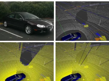
B. Detection of Black Obstacles

Laser range finders are widely known to have difficulty seeing black objects. Since these objects absorb light, the sensor never gets a return. Clearly it is desirable to “see” black obstacles for driving applications. Other sensors could be used, but they all have their own drawbacks. Here we

Fig. 10. Detecting black vehicles in 3D range scans. White points represent raw Velodyne data. Yellow lines represent the generated virtual scans. Top left: actual appearance of the vehicle. Top right: the vehicle gives very few laser returns. Bottom left: virtual scan with black object detection. Bottom right: virtual scan without black object detection.

present a method for detecting black objects in 3D laser data. Figure 10 shows the returns obtained from a black car. The only readings obtained are from the license plate and wheels of the vehicle, all of which get filtered out as low obstacles. Instead of looking at the little data that is present, we can detect the black obstacle by looking at the data that is absent. If no readings are obtained along a range of vertical angles in a specific direction, we can conclude that the space must be occupied by a black obstacle. Otherwise the rays would have hit some obstacle or the ground. To provide a conservative estimate of the range to the black obstacle we place it at the last reading obtained in the vertical angles just before the absent readings. We note that this method works well as long as the sensor is good at seeing the ground. For the Velodyne sensor the range within which the ground returns are reliable is about 25 - 30m, beyond this range the black obstacle detection logic does not work.

VI. EXPERIMENTALVALIDATION

The most challenging traffic situation at the Urban Grand Challenge was presented on course A during the qualifying event (Fig. 11) . The test consisted of dense human driven traffic in both directions on a course with an outline resem-bling the Greek letterθ. The robots had to merge repeatedly into the dense traffic. The merge was performed using a left turn, so that the robots had to cross one lane of traffic each time. In these conditions accurate estimates of positions and velocities of the cars are very useful for determining a gap in traffic large enough to perform the merge safely. Cars passed in close proximity to each other and to station-ary obstacles (e.g. signs and guard rails) providing plenty of opportunity for false associations. Partial and complete occlusions happened frequently due to the traffic density. Moreover these occlusions often happened near merge points which complicated decision making.

During extensive testing, the performance of our vehicle tracking module has been very reliable and efficient (see Fig. 11). Geometric shape of vehicles was properly estimated (see Figs. 12 and 13), which increased tracking reliability and improved motion estimation. The tracking approach proved

(a) actual scene (b) Velodyne data

(c) after classification (d) generated virtual scan

Fig. 9. In (c) Velodyne data is colored by type: orange - ground, yellow - low obstacle, red - medium obstacle, green - high obstacle. In (d) yellow lines denote the virtual scan. Note the truck crossing the intersection, the cars parked on a side of the road and the white van parked on a driveway. On the virtual scan all of these vehicles are clearly marked as obstacles, but ground, curbs and tree tops are ignored.

TABLE I

TRACKER PERFORMANCE ON DATA SETS FROM THREE URBAN ENVIRONMENTS. MAXTPIS THE THEORETICALLY MAXIMUM POSSIBLE TRUE POSITIVE PERCENT FOR EACH DATA SET. TPANDFPARE THE ACTUAL TRUE POSITIVE AND FALSE POSITIVE RATES ATTAINED BY THE ALGORITHM.

Total Total Correctly Falsely Max TP TP FP Data Sets Frames Vehicles Identified Identified (%) (%) (%)

UGC Area A 1,577 5,911 5,676 205 97.8 96.02 3.35

Stanford Campus 2,140 3,581 3,530 150 99.22 98.58 4.02

Alameda Day 1 1,531 901 879 0 98.22 97.56 0

Overall 5,248 10,393 10,085 355 98.33 97.04 3.3

capable of handling complex traffic situations such as the one presented on course A of the UGC. The computation time of our approach averages at 25ms per frame, which is faster than real time for most modern laser range finders.

We also gathered empirical results of the tracking module performance on data sets from several urban environments: course A of the UGC, Stanford campus and a port town in Alameda, CA. For each frame of data we counted how many vehicles a human is able to identify in the laser range data. The vehicles had to be within 50m of the ego-vehicle, on or near the road, and moving with a speed of at least 5mph. We summarize the tracker’s performance in Tbl. I. Note that the maximum theoretically possible true positive rate is lower than 100% because three frames are required to detect a new vehicle. On all three data sets the tracker performed very close to the theoretical bound. Overall the true positive rate was97%compared to the theoretical maximum of98%. Several videos of vehicle detection and tracking using the techniques presented in this paper are available at the website

http://cs.stanford.edu/people/petrovsk/uc.html

VII. CONCLUSIONS

We have presented the vehicle tracking module developed for Stanford’s autonomous driving robot Junior. Tracking is performed from a high-speed moving platform and relies on laser range finders for sensing. Our approach models both dynamic and geometric properties of the tracked vehicles and estimates them with a single Bayes filter per vehicle. In contrast to prior art, the common data segmentation and association steps are carried out as part of the filter itself. The approach has proved reliable, efficient and capable of handling challenging traffic situations, such as the ones presented at the Urban Grand Challenge.

Clearly there is ample room for future work. The pre-sented approach does not model pedestrians, bicyclists, or motorcyclists, which is a prerequisite for driving in populated areas. Another promising direction for future work is fusion of different sensors, including laser, radar and vision.

VIII. ACKNOWLEDGEMENTS

This research has been conducted for the Stanford Racing Team and would have been impossible without the whole team’s efforts to build the hardware and software that makes up the team’s robot Junior. The authors thank all team

(a)

(b)

(c)

Fig. 11. Tracking results on course A at the UGC. (a) actual scene, (b) Velodyne data, (c) virtual scan and tracking results. In (c) yellow line segments represent the virtual scan and red/green/white points show results of scan differencing. The purple boxes denote the tracked vehicles. (Best viewed in color.)

Fig. 12. Size estimation results on Stanford campus. Vehicles of different sizes are successfully estimated and tracked. (Best viewed in color.)

(a) without size estimation (b) with size estimation Fig. 13. Size estimation improves accuracy of tracking as can be seen on the example of a passing bus taken from an Alameda data set. Without size estimation (a) the tracking results are poor because the geometric model does not fit the data well. Not only is the velocity estimated incorrectly, but the track is lost entirely when the bus is passing. With size estimation (b) the bus is tracked successfully and the velocity is properly estimated. (Best viewed in color.)

members for their hard work. The Stanford Racing Team is indebted to DARPA for creating the Urban Challenge, and for its financial support under the Track A Program. Further, Stanford University thanks its various sponsors. Special thanks also to NASA Ames for permission to use their air field.

REFERENCES

[1] M. Buehler, K. Iagnemma, and S. Singh, The 2005 Darpa Grand

Challenge: The Great Robot Race. Springer Verlag, 2007. [2] DARPA, Urban challenge rules, revision oct. 27, 2007. See

www.darpa.mil/grandchallenge/rules.asp, 2007.

[3] M. Montemerlo, J. Becker, S. Bhat, H. Dahlkamp, D. Dolgov, S. Et-tinger, D. Haehnel, T. Hilden, G. Hoffmann, B. Huhnke, et al., “Junior: The Stanford entry in the Urban Challenge,” Journal of Field Robotics, vol. 25, no. 9, pp. 569–597, 2008.

[4] T. Zielke, M. M. Brauckmann, and W. v. Seelen, “Intensity and edge based symmetry detection applied to car following,” in ECCV, Berlin,

Germany, 1992.

[5] E. Dickmanns, “Vehicles capable of dynamic vision,” in IJCAI,

Nagoya, Japan, 1997.

[6] F. Dellaert and C. Thorpe, “Robust car tracking using kalman filtering and bayesian templates,” in Conference on Intelligent Transportation

Systems, 1997.

[7] L. Zhao and C. Thorpe, “Qualitative and quantitative car tracking from a range image sequence,” in Computer Vision and Pattern Recognition, 1998.

[8] D. Streller, K. Furstenberg, and K. Dietmayer, “Vehicle and object models for robust tracking in traffic scenes using laser range images,” in Intelligent Transportation Systems, 2002.

[9] C. Wang, C. Thorpe, S. Thrun, M. Hebert, and H. Durrant-Whyte, “Simultaneous localization, mapping and moving object tracking,” The

International Journal of Robotics Research, Sep 2007; vol. 26: pp. 889-916, 2007.

[10] S. Wender and K. Dietmayer, “3d vehicle detection using a laser scanner and a video camera,” in 6th European Congress on ITS,

Aalborg, Denmark, 2007.

[11] S. S. Blackman, “Multiple hypothesis tracking for multiple target tracking,” IEEE AE Systems Magazine, 2004.

[12] S¨arkk¨a, S. and Vehtari, A. and Lampinen, J., “Rao-blackwellized particle filter for multiple target tracking,” Inf. Fusion, vol. 8, no. 1, 2007.

[13] D. Schulz, W. Burgard, D. Fox, and A. Cremers, “Tracking multiple moving targets with a mobile robot using particle filters and statistical data association,” in ICRA, 2001.

[14] A. Petrovskaya and S. Thrun, “Efficient techniques for dynamic vehicle detection,” in ISER, Athens, Greece, 2008.

[15] A. Petrovskaya and S. Thrun, “Model based vehicle tracking for au-tonomous driving in urban environments,” in RSS, Zurich, Switzerland, 2008.

[16] A. Doucet, N. d. Freitas, K. Murphy, and S. Russell, “Rao-blackwellised filtering for dynamic bayesian networks,” in UAI, San