Tracking-Learning-Detection

Tracking-Learning-Detection

Zdenek Kalal, Krystian Mikolajczyk, and Jiri Matas,

Abstract—This paper investigates long-term tracking of unknown objects in a video stream. The object is defined by its location and extent in a single frame. In every frame that follows, the task is to determine the object’s location and extent or indicate that the object is not present. We propose a novel tracking framework (TLD) that explicitly decomposes the long-term tracking task into tracking, learning and detection. The tracker follows the object from frame to frame. The detector localizes all appearances that have been observed so far and corrects the tracker if necessary. The learning estimates detector’s errors and updates it to avoid these errors in the future. We study how to identify detector’s errors and learn from them. We develop a novel learning method (P-N learning) which estimates the errors by a pair of “experts”: (i) P-expert estimates missed detections, and (ii) N-expert estimates false alarms. The learning process is modeled as a discrete dynamical system and the conditions under which the learning guarantees improvement are found. We describe our real-time implementation of the TLD framework and the P-N learning. We carry out an extensive quantitative evaluation which shows a significant improvement over state-of-the-art approaches.

Index Terms—Long-term tracking, learning from video, bootstrapping, real-time, semi-supervised learning

F

1

I

Consider a video stream taken by a hand-held camera depict-ing various objects movdepict-ing in and out of the camera’s field of view. Given a bounding box defining the object of interest in a single frame, our goal is to automatically determine the object’s bounding box or indicate that the object is not visible in every frame that follows. The video stream is to be processed at frame-rate and the process should run indefinitely long. We refer to this task as long-term tracking.

To enable the long-term tracking, there are a number of problems which need to be addressed. The key problem is the detection of the object when it reappears in the camera’s field of view. This problem is aggravated by the fact that the object may change its appearance thus making the appearance from the initial frame irrelevant. Next, a successful long-term tracker should handle scale and illumination changes, background clutter, partial occlusions and operate in real-time. The long-term tracking can be approached either from tracking or from detection perspectives. Tracking algorithms estimate the object motion. Trackers require only initialization, are fast and produce smooth trajectories. On the other hand, they accumulate error during run-time (drift) and typically fail if the object disappears from the camera view. Research in tracking aims at developing increasingly robust trackers that track “longer”. The post-failure behavior is not directly addressed. Detection-based algorithms estimate the object lo-cation in every frame independently. Detectors do not drift and do not fail if the object disappears from the camera view. However, they require an offline training stage and therefore cannot be applied to unknown objects.

• Z. Kalal and K. Mikolajczyk are with the Centre for Vision, Speech and Signal Processing, University of Surrey, Guildford, UK.

WWW: http://info.ee.surrey.ac.uk/Personal/Z.Kalal/

• J. Matas is with the Center for Machine Perception, Department of Cybernetics, Faculty of Electrical Engineering, Czech Technical University in Prague, Czech Republic.

The starting point of our research is the acceptance of the fact that neither tracking nor detection can solve the long-term tracking task independently. However, if they operate simultaneously, there is potential to benefit one from another. A tracker can provide weakly labeled training data for a detector and thus improve it during run-time. A detector can re-initialize a tracker and thus minimize the tracking failures. The first contribution of this paper is the design of a novel framework (TLD) that decomposes the long-term tracking task into three sub-tasks: tracking, learning and detection. Each sub-task is addressed by a single component and the compo-nents operate simultaneously. The tracker follows the object from frame to frame. The detector localizes all appearances that have been observed so far and corrects the tracker if necessary. The learning estimates detector’s errors and updates it to avoid these errors in the future.

While a wide range of trackers and detectors exist, we are not aware of any learning method that would be suitable for the TLD framework. Such a learning method should: (i) deal with arbitrarily complex video streams where the tracking failures are frequent, (ii) never degrade the detector if the video does not contain relevant information and (iii) operate in real-time. To tackle all these challenges, we rely on the various information sources contained in the video. Consider, for instance, a single patch denoting the object location in a single frame. This patch defines not only the appearance of the object, but also determines the surrounding patches, which define the appearance of the background. When tracking the patch, one can discover different appearances of the same object as well as more appearances of the background. This is in contrast to standard machine learning approaches, where a single example is considered independent from other examples [1]. This opens interesting questions how to effectively exploit the information in the video during learning.

The second contribution of the paper is the new learning paradigm called P-N learning. The detector is evaluated in every frame of the video. Its responses are analyzed by two

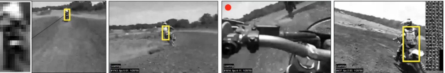
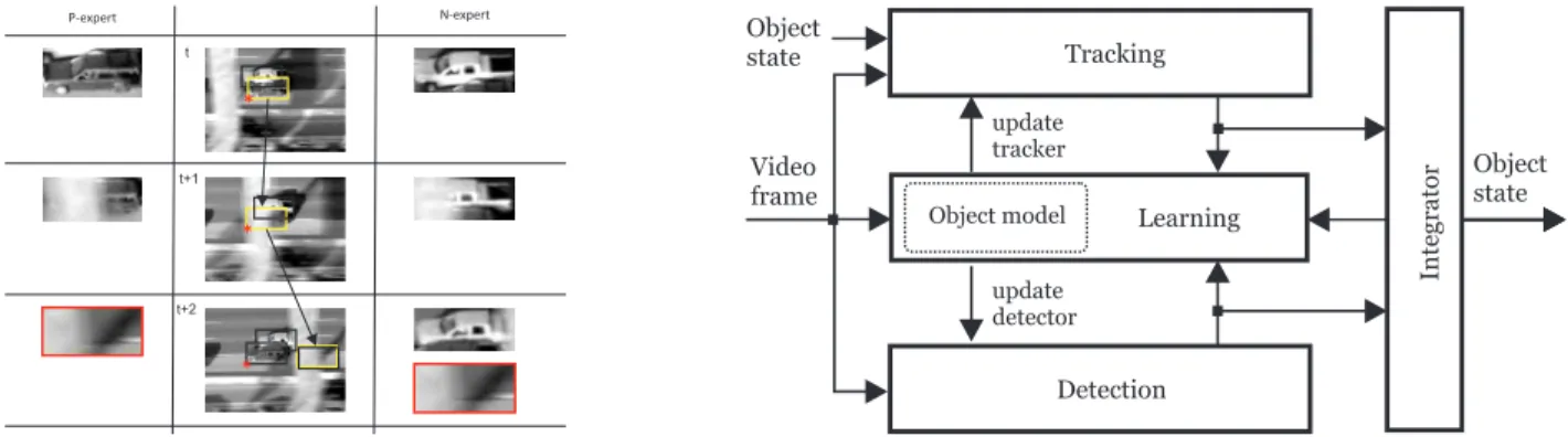
Fig. 1. Given a single bounding box defining the object location and extent in the initial frame (LEFT), our system tracks, learns and detects the object in real-time. The red dot indicates that the object is not visible.

types of ”experts”: (i)P-expert– recognizes missed detections, and (ii) N-expert – recognizes false alarms. The estimated errors augment a training set of the detector, and the detector is retrained to avoid these errors in the future. As any other process, also the P-N experts are making errors them self. However, if the probability of expert’s error is within certain limits (which will be analytically quantified), the errors are mutually compensated which leads to stable learning.

The third contribution is the implementation. We show how to build a real-time long-term tracking system based on the TLD framework and the P-N learning. The system tracks, learns and detects an object in a video stream in real-time.

The fourth contribution is the extensive evaluation of the state-of-the-art methods on benchmark data sets, where our method achieved saturated performance. Therefore, we have collected and annotated new, more challenging data sets, where a significant improvement over state-of-the-art was achieved.

The rest of the paper is organized as follows. Section 2 reviews the work related to the long-term tracking. Section 3 introduces the TLD framework and section 4 proposes the P-N learning. Section 5 comments on the implementation of TLD. Section 6 then performs a number of comparative experiments. The paper finishes with contributions and suggestions for future research.

2

R

This section reviews the related approaches for each of the component of our system. Section 2.1 reviews the object tracking with the focus on robust trackers that perform online learning. Section 2.2 discusses the object detection. Finally, section 2.3 reviews relevant machine learning approaches for training of object detectors.

2.1 Object tracking

Object tracking is the task of estimation of the object motion. Trackers typically assume that the object is visible through-out the sequence. Various representations of the object are used in practice, for example: points [2], [3], [4], articulated models [5], [6], [7], contours [8], [9], [10], [11], or optical flow [12], [13], [14]. Here we focus on the methods that represent the objects by geometric shapes and their motion is estimated between consecutive frames, i.e. the so-called frame-to-frame tracking. Template tracking is the most straightfor-ward approach in that case. The object is described by a target template (an image patch, a color histogram) and the motion is

defined as a transformation that minimizes mismatch between the target template and the candidate patch. Template tracking can be either realized as static [15] (when the target template does not change), or adaptive [2], [3] (when the target template is extracted from the previous frame). Methods that combine static and adaptive template tracking have been proposed [16], [17], [18], as well as methods that recognize ”reliable” parts of the template [19], [20]. Templates have limited modeling capabilities as they represent only a single appearance of the object. To model more appearance variations, the generative models have been proposed. The generative models are either build offline [21], or during run-time [22], [23]. The generative trackers model only the appearance of the object and as such often fail in cluttered background. In order to alleviate this problem, recent trackers also model the environment where the object moves. Two approaches to environment modeling are often used. First, the environment is searched for supporting object the motion of which is correlated with the object of in-terest [24], [25]. These supporting object then help in tracking when the object of interest disappears from the camera view or undergoes a difficult transformation. Second, the environment is considered as a negative class against which the tracker should discriminate. A common approach of discriminative trackers is to build a binary classifier that represents the deci-sion boundary between the object and its background. Static discriminative trackers [26] train an object classifier before tracking which limits their applications to known objects. Adaptive discriminative trackers [27], [28], [29], [30] build a classifier during tracking. The essential phase of adaptive discriminative trackers is the update: the close neighborhood of the current location is used to sample positive training examples, distant surrounding of the current location is used to sample negative examples, and these are used to update the classifier in every frame. It has been demonstrated that this updating strategy handles significant appearance changes, short-term occlusions, and cluttered background. However, these methods also suffer from drift and fail if the object leaves the scene for longer than expected. To address these problems the update of the tracking classifier has been constrained by an auxiliary classifier trained in the first frame [31] or by training a pair of independent classifiers [32], [33].

2.2 Object detection

Object detection is the task of localization of objects in an input image. The definition of an ”object” vary. It can be a single instance or a whole class of objects. Object detection

methods are typically based on the local image features [34] or a sliding window [35]. The feature-based approaches usu-ally follow the pipeline of: (i) feature detection, (ii) feature recognition, and (iii) model fitting. Planarity [34], [36] or a full 3D model [37] is typically exploited. These algorithms reached a level of maturity and operate in real-time even on low power devices [38] and in addition enable detection of a large number of objects [39], [40]. The main strength as well as the limitation is the detection of image features and the requirement to know the geometry of the object in advance. The sliding window-based approaches [35], scan the input image by a window of various sizes and for each window decide whether the underlying patch contains the object of interest or not. For a QVGA frame, there are roughly 50,000 patches that are evaluated in every frame. To achieve a real-time performance, sliding window-based detectors adopted the so-called cascaded architecture [35]. Exploiting the fact that background is far more frequent than the object, a classifier is separated into a number of stages, each of which enables early rejection of background patches thus reducing the number of stages that have to be evaluated on average. Training of such detectors typically requires a large number of training examples and intensive computation in the training stage to accurately represent the decision boundary between the object and background. An alternative approach is to model the object as a collection of templates. In that case the learning involves just adding one more template [41].

2.3 Machine learning

Object detectors are traditionally trained assuming that all training examples are labeled. Such an assumption is too strong in our case since we wish to train a detector from a single labeled example and a video stream. This problem can be formulated as a semi-supervised learning [42], [43] that exploits both labeled and unlabeled data. These methods typically assume independent and identically distributed data with certain properties, such as that the unlabeled examples form “natural” clusters in the feature space. A number of algorithms relying on similar assumptions have been proposed in the past including EM, Self-learning and Co-training.

Expectation-Maximization (EM) is a generic method for finding estimates of model parameters given unlabeled data. EM is an iterative process, which in case of binary classifica-tion alternates over estimaclassifica-tion of soft-labels of unlabeled data and training a classifier. EM was successfully applied to docu-ment classification [44] and learning of object categories [45]. In the semi-supervised learning terminology, EM algorithm relies on the ”low density separation” assumption [42], which means that the classes are well separated. EM is sometimes interpreted as a “soft” version of self-learning [43].

Self-learning starts by training an initial classifier from a labeled training set, the classifier is then evaluated on the unlabeled data. The examples with the most confident classifier responses are added to the training set and the classifier is retrained. This is an iterative process. The self-learning has been applied to human eye detection in [46]. However, it was observed that the detector improved more if the unlabeled

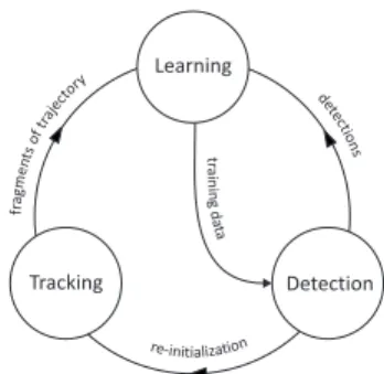
Fig. 2. The block diagram of the TLD framework.

data was selected by an independent measure rather than the classifier confidence. It was suggested that the low density separation assumption is not satisfied for object detection and other approaches may work better.

Co-training [1] is a learning method build on the idea that independent classifiers can mutually train one another. To create such independent classifiers, co-training assumes that two independent feature-spaces are available. The learning is initialized by training of two separate classifiers using the labeled examples. Both classifiers are then evaluated on unlabeled data. The confidently labeled samples from the first classifier are used to augment the training set of the second classifier and vice versa in an iterative process. Co-training works best for problems with independent modalities, e.g. text classification [1] (text and hyper-links) or biometric recognition systems [47] (appearance and voice). In visual object detection, co-training has been applied to car detection in surveillance [48] and moving object recognition [49]. We argue that co-training is suboptimal for object detection, since the examples (image patches) are sampled from a single modality. Features extracted from a single modality may be dependent and therefore violate the assumptions of co-training.

2.4 Most related approaches

Many approaches combine tracking, learning and detection in some sense. In [50], an offline trained detector is used to validate the trajectory output by a tracker and if the trajectory is not validated, an exhaustive image search is performed to find the target. Other approaches integrate the detector within a particle filtering [51] framework. Such techniques have been applied to tracking of faces in low frame-rate video [52], multiple hockey players [53], or pedestrians [54], [55]. In contrast to our method, these methods rely on an offline trained detector that does not change its properties during run-time. Adaptive discriminative trackers [29], [30], [31], [32], [33] also have the capability to track, learn and detect. These methods realize tracking by an online learned detector that discriminates the target from its background. In other words, a single process represents both tracking and detection. This is in contrast to our approach where tracking and detection are independent processes that exchange information using learning. By keeping the tracking and detection separated our approach does not have to compromise neither on tracking nor detection capabilities of its components.

Training P-N experts Classifier unlabeled data Training Set labeled data labels classifier parameters [+] examples [-] examples

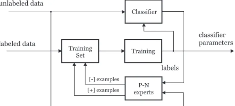
Fig. 3. The block diagram of the P-N learning.

3

T

-L

-D

TLD is a framework designed for long-term tracking of an unknown object in a video stream. Its block diagram is shown in figure 2. The components of the framework are characterized as follows:Trackerestimates the object’s motion between consecutive frames under the assumption that the frame-to-frame motion is limited and the object is visible. The tracker is likely to fail and never recover if the object moves out of the camera view. Detector treats every frame as independent and performs full scanning of the image to localize all appearances that have been observed and learned in the past. As any other detector, the detector makes two types of errors: false positives and false negative. Learning observes performance of both, tracker and detector, estimates detector’s errors and generates training examples to avoid these errors in the future. The learning component assumes that both the tracker and the detector can fail. By the virtue of the learning, the detector generalizes to more object appearances and discriminates against background.

4

P-N

This section investigates the learning component of the TLD framework. The goal of the component is to improve the performance of an object detector by online processing of a video stream. In every frame of the stream, we wish to evaluate the current detector, identify its errors and update it to avoid these errors in the future. The key idea of P-N learning is that the detector errors can be identified by two types of “experts”. P-expert identifies only false negatives, N-expert identifies only false positives. Both of the N-experts make errors themselves, however, their independence enables mutual compensation of their errors.

Section 4.1 formulates the P-N learning as a semi-supervised learning method. Section 4.2 models the P-N learn-ing as a discrete dynamical system and finds conditions under which the learning guarantees improvement of the detector. Section 4.3 performs several experiments with synthetically generated experts. Finally, section 4.4 applies the P-N learning to training object detectors from video and proposes experts that could be used in practice.

4.1 Formalization

Letxbe an example from a feature-spaceX andy be a label from a space of labels Y = {−1,1}. A set of examples X

is called an unlabeled set, Y is called a set of labels and L = {(x, y)} is called a labeled set. The input to the P-N learning is a labeled set Ll and an unlabeled set Xu, where l u. The task of P-N learning is to learn a classifier f : X → Y from labeled set Ll and bootstrap its performance by the unlabeled set Xu. Classifier f is a function from a family F parameterized by Θ. The family F is subject to implementation and is considered fixed in training, the training therefore corresponds to estimation of the parametersΘ.

The P-N learning consists of four blocks: (i) aclassifierto be learned, (ii) training set – a collection of labeled training examples, (iii) supervised training – a method that trains a classifier from training set, and (iv) P-N experts – functions that generate positive and negative training examples during learning. See figure 3 for illustration.

The training process is initialized by inserting the labeled set L to the training set. The training set is then passed to supervised learning which trains a classifier, i.e. estimates the initial parametersΘ0_{. The learning process then proceeds by}

iterative bootstrapping. In iterationk, the classifier trained in previous iteration classifies the entire unlabeled set, yk

u = f(xu|Θk−1) for all xu ∈ Xu. The classification is analyzed by the P-N experts which estimate examples that have been classified incorrectly. These examples are added with changed labels to the training set. The iteration finishes by retraining the classifier, i.e. estimation ofΘk. The process iterates until convergence or other stopping criterion.

The crucial element of P-N learning is the estimation of the classifier errors. The key idea is to separate the estimation of false positives from the estimation of false negatives. For this reason, the unlabeled set is split into two parts based on the current classification and each part is analyzed by an independent expert. P-expert analyzes examples classified as negative, estimates false negatives and adds them to training set with positive label. In iterationk, P-expert outputs n+_(k)

positive examples. N-expert analyzes examples classified as positive, estimates false positives and adds them with neg-ative label to the training set. In iteration k, the N-expert outputsn−(k) negative examples. The P-expert increases the classifier’s generality. The N-expert increases the classifier’s discriminability.

Relation to supervised bootstrap.To put the P-N learning

into broader context, let us consider that the labels of set Xu are known. Under this assumption it is straightforward to recognize misclassified examples and add them to the training set with correct labels. Such a strategy is commonly called (supervised) bootstraping [56]. A classifier trained using such supervised bootstrap focuses on the decision boundary and often outperforms a classifier trained on randomly sampled training set [56]. The same idea of focusing on the decision boundary underpins the P-N learning with the difference that the labels of the set Xu are unknown. P-N learning can therefore be viewed as a generalization of standard bootstrap to unlabeled case where labels are not given but ratherestimated using the N experts. As any other process, also the P-N experts make errors by estimating the labels incorrectly. Such errors propagate through the training, which will be theoretically analyzed in the following section.

4.2 Stability

This section analyses the impact of the P-N learning on the classifier performance. We assume an abstract classifier (e.g. nearest neighbour) the performance of which is measured on Xu. The classifier initially classifies the unlabeled set at random and then corrects its classification for those examples that were returned by the P-N experts. For the purpose of the analysis, let us consider that the labels ofXu are known. This will allow us to measure both the classifier errors and the errors of the P-N experts. The performance of this classifier will be characterized by a number of false positivesα(k)and a number of false negativesβ(k), wherekindicates the iteration of training.

In iterationk, the P-expert outputsn+

c(k)positive examples which are correct (positive based on the ground truth), and n+_f(k) positive examples which are false (negative based on the ground truth), which forces the classifier to change n+(k) = n+_c(k) + n+_f(k) negatively classified examples to positive. Similarly, the N-experts outputs n−_c(k) correct negative examples andn−_f(k)false negative examples, which forces the classifier to change n−(k) = n−c(k) + n−f(k) examples classified as positive to negative. The false positive and false negative errors of the classifier in the next iteration thus become:

α(k+ 1) =α(k)−n_c−(k) +n+_f(k) (1a) β(k+ 1) =β(k)−n_c+(k) +n−_f(k). (1b) Equation 1a shows that false positives α(k) decrease if n−c(k)> n

+

f(k), i.e. number of examples that were correctly relabeled to negative is higher than the number of examples that were incorrectly relabeled to positive. Similarly, the false negativesβ(k)decrease ifn+

c(k)> n−f(k).

Quality measures. In order to analyze the convergence of

the P-N learning, a model needs to be defined that relates the quality of the P-N experts to the absolute number of positive and negative examples output in each iteration. The quality of the P-N experts is characterized by four quality measures:

• P-precision – reliability of the positive labels, i.e. the number of correct positive examples divided by the number of all positive examples output by the P-expert, P+=n+_c/(n+_c +n+_f).

• P-recall – percentage of identified false negative errors, i.e. the number of correct positive examples divided by the number of false negatives output by the classifier, R+_=n+

c/ β.

• N-precision– reliability of negative labels, i.e. the number of correct negative examples divided by the number of all positive examples output by the N-expert, P− =

n−_c /(n−_c +n−_f).

• N-recall – percentage of recognized false positive errors, i.e. the number of correct negative examples divided by the number of all false positives output by the classifier, R−=n−_c/ α.

Given these quality measures, the number of correct and false examples output by P-N experts at iteration k have the

l1=0,l2< 1

a

b b b

a a

l1=0,l2=1 l1=0,l2> 1

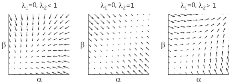
Fig. 4. Evolution of errors during P-N learning for differ-ent eigenvalues of matrixM. The errors are decreasing (LEFT), are static (MIDDLE) or grow (RIGHT).

following form: n+_c(k) =R+β(k), n+_f(k) =(1−P +₎ P+ R +_{β(k) (2a)} n−_c(k) =R−α(k), n−_f(k) = (1−P −₎ P− R −_{α(k). (2b)}

By combining the equation 1a, 1b, 2a and 2b we obtain the following equations: α(k+ 1) = (1−R−)α(k) +(1−P +₎ P+ R +_{β(k) (3a)} β(k+ 1) =(1−P −₎ P− R −_{α(k) + (1−R}+_)β(k). (3b) After defining the state vector~x(k) =

α(k) β(k)T and a 2×2matrix Mas M= " 1−R− (1−P+₎ P+ R + (1−P−₎ P− R− (1−R +₎ # (4)

it is possible to rewrite the equations as ~

x(k+ 1) =M~x(k).

This is a recursive equations that correspond to a discrete dynamical system. The system shows how the error of the classifier (encoded by the system state) propagates from one iteration of P-N learning to another. Our goal is to show, under which conditions the error in the system drops.

Based on the well founded theory of dynamical systems [57], [58], the state vector~xconverges to zero if both eigen-valuesλ1, λ2of the transition matrixMare smaller than one.

Note that the matrix M is a function of the expert’s quality measures. Therefore, if the quality measures are known, it allows the determine the stability of the learning. Experts for which corresponding matrix M has both eigenvalues smaller than one will be called error-canceling. Figure 4 illustrates the evolution of error of the classifier when λ1 = 0 and (i)

λ2<1, (ii)λ2= 1, (iii) λ2>1.

In the above analysis the quality measures were assumed to be constant and the classes separable. In practice, it is not not possible to identify all the errors of the classifier. Therefore, the training does not converge to error-less classifier, but may stabilize at a certain level. In case the quality measure vary, the performance increases in those iterations where the eigenvalues ofM are smaller than one.

0 1000

0

1

Number of Frames Processed

F-Measure

0.0 0.5

0.6

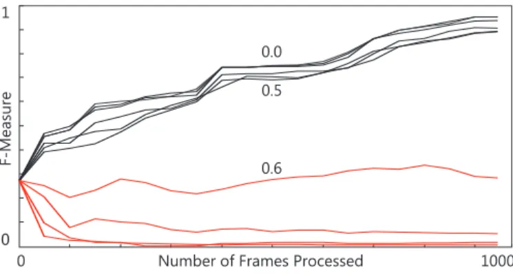
Fig. 5. Performance of a detector as a function of the number of processed frames. The detectors were trained by synthetic P-N experts with certain level of error. The classifier is improved up to error 50% (BLACK), higher error degrades it (RED).

4.3 Experiments with simulated experts

In this experiment, a classifier is trained on a real sequence using simulated P-N experts. Our goal is to analyze the learning performance as a function of the expert’s quality measures.

The analysis is carried on sequence CAR (see figure 12). In the first frame of the sequence, we train a random forrest classifier using affine warps of the initial patch and the back-ground from the first frame. Next, we perform a single run over the sequence. In every frame, the classifier is evaluated, the simulated experts identify errors and the classifier is updated. After every update, the classifier is evaluated on the entire sequence to measure its performance using f-measure. The performance is then drawn as a function of the number of processed frames and the quality of the P-N experts.

The P-N experts are characterized by four quality measures, P+_{, R}+_{, P}−_{, R}−_{. To reduce this 4D space, the parameters are}

set to P+ _=R+ _{= P}− _=R− _{= 1−, where represents}

error of the expert. The transition matrix then becomesM=

1, where1is a 2x2 matrix with all elements equal to 1. The eigenvalues of this matrix areλ1= 0, λ2= 2. Therefore the

P-N learning should be improving the performance if <0.5. The error is varied in the range= 0 : 0.9.

The experts are simulated as follows. In framek, the classi-fier generatesβ(k)false negatives. P-expert relabelsn+

c(k) =

(1−)β(k)of them to positive which gives R+_{= 1−. In}

order to simulate the required precision P+ _{= 1−, the}

P-expert relabels additionaln+_f(k) = β(k)background samples to positive. Therefore, the total number of examples relabeled to positive in iterationkisn+_=n+

c(k) +n

+

f(k) =β(k). The N-experts were generated similarly.

The performance of the detector as a function of number of processed frames is depicted in figure 5. Notice that if≤0.5

the performance of the detector increases with more training data. In general,= 0.5will give unstable results although in this sequence it leads to improvements. Increasing the noise-level further leads to sudden degradation of the classifier. These results are in line with the P-N Learning theory.

a) scanning grid b) unacceptable labeling c) acceptable labeling

Fig. 6. Illustration of a scanning grid and corresponding volume of labels. Red dots correspond to positive labels.

4.4 Design of real experts

This section applies the P-N learning to training an object detector from a labeled frame and a video stream. The de-tector consists of a binary classifier and a scanning window, and the training examples correspond to image patches. The labeledexamplesXlare extracted from the labeled frame. The unlabeled dataXu are extracted from the video stream.

The P-N learning is initialized by supervised training of so-called initial detector. In every frame, the P-N learning performs the following steps: (i) evaluation of the detector on the current frame, (ii) estimation of the detector errors using the P-N experts, (iii) update of the detector by labeled examples output by the experts. The detector obtained at the end of the learning is called thefinal detector.

Figure 6 (a) that shows three frames of a video sequence overlaid with a scanning grid. Every bounding box in the grid defines an image patch, the label of which is represented as a colored dot in (b,c). Every scanning window-based detector considers the patches as independent. Therefore, there are2N possible label combinations in a single frame, whereN is the number of bounding boxes in the grid. Figure 6 (b) shows one such labeling. The labeling indicates, that the object appears in several locations in a single frame and that there is no temporal continuity in the motion. Such labeling is unlikely to be correct. On the other hand, if the detector outputs results depicted in (c) the labeling is plausible since the object appears at one location in each frame and the detected locations build up a trajectory in time. In other words, the labels of the patches are dependent. We refer to such a property as structure. The key idea of the P-N experts is to exploit the structure in data to identify the detector errors.

P-expert exploits the temporal structure in the video and

assumes that the object moves along a trajectory. The P-expert remembers the location of the object in the previous frame and estimates the object location in current frame using a frame-to-frame tracker. If the detector labeled the current location as negative (i.e. made false negative error), the P-expert generates a positive example.

N-expert exploits the spatial structure in the video and

assumes that the object can appear at a single location only. The N-expert analyzes all responses of the detector in the current frame and the response produced by the tracker and selects the one that is the most confident. Patches that are not overlapping with the maximally confident patch are labeled as negative. The maximally confident patch re-initializes the location of the tracker.

Fig. 7. Illustration of the examples output by the P-N experts. The third row shows error compensation.

to be learned is a car within the yellow bounding box. The car is tracked from frame to frame by a tracker. The tracker represents the P-expert that outputs positive training examples. Notice that due to occlusion of the object, the output of P-expert in time t+ 2 outputs incorrect positive example. N-expert identifies maximally confident patch (denoted by a red star) and labels all other detections as negative. Notice that the N-expert is discriminating against another car, and in addition corrected the error made by the P-expert in time t+ 2.

5

I

TLD

This section describes our implementation of the TLD frame-work. The block diagram is shown in figure 8.

5.1 Prerequisites

At any time instance, the object is represented by its state. The state is either a bounding box or a flag indicating that the object is not visible. The bounding box has a fixed aspect ratio (given by the initial bounding box) and is parameterized by its location and scale. Other parameters such as in-plane rotation are not considered. Spatial similarity of two bounding boxes is measured using overlap, which is defined as a ratio between intersection and union.

A single instance of the object’s appearance is represented by an image patch p. The patch is sampled from an image within the object bounding box and then is re-sampled to a normalized resolution (15x15 pixels) regardless of the aspect ratio. Similarity between two patchespi, pj is defined as

S(pi, pj) = 0.5(NCC(pi, pj) + 1), (5) where NCC is a Normalized Correlation Coefficient.

A sequence of object states defines atrajectoryof an object in a video volume as well as the corresponding trajectory in the appearance (feature) space. Note that the trajectory is fragmented as the object may not be visible.

5.2 Object model

Object model M is a data structure that represents the object and its surrounding observed so far. It is a collection of positive and negative patches, M =

Tracking Detection Integrator Object state Learning update detector Video frame Object model Object state update tracker

Fig. 8. Detailed block diagram of the TLD framework.

{p+₁, p+₂, . . . , p+

m, p

−

1, p

−

2, . . . , p−n}, where p+ and p− repre-sent the object and background patches, respectively. Positive patches areorderedaccording to the time when the patch was added to the collection. p+₁represents the first positive patch added to the collection,p+

mis the positive patch added last. Given an arbitrary patchpand object modelM, we define several similarity measures:

1) Similarity with the positive nearest neighbor, S+(p, M) = max_p+

i∈MS(p, p

+

i ).

2) Similarity with the negative nearest neighbor, S−(p, M) = max_p−

i∈MS(p, p

−

i ).

3) Similarity with the positive nearest neighbor consid-ering 50% earliest positive patches, S_50%+ (p, M) = max_p+ i∈M V_i<m 2 S(p, p + i ). 4) Relative similarity, Sr ₌ S+ S+_+S−. Relative similarity

ranges from 0 to 1, higher values mean more confident that the patch depicts the object.

5) Conservative similarity, Sc ₌ S50%+ S+

50%+S−

. Conservative similarity ranges from 0 to 1. High value of Sc _mean more confidence that the patch resembles appearance observed in the first 50% of the positive patches.

Nearest Neighbor (NN) classifier.The similarity measures

(Sr, Sc) are used throughout TLD to indicate how much an arbitrary patch resembles the appearances in the model. The Relative similarity is used to define a nearest neighbor classifier. A patchpis classified as positive ifSr(p, M)> θNN

otherwise the patch is classified as negative. A classification margin is defined asSr_{(p, M)−θ}

NN. Parameter θNN enables

tuning the NN classifier either towards recall or precision.

Model update. To integrate a new labeled patch to the

object model we use the following strategy: the patch is added to the collection only if the its label estimated by NN classifier is different from the label given by the P-N experts. This leads to a significant reduction of accepted patches at the cost of coarser representation of the decision boundary. Therefore we improve this strategy by adding also patches where the classification margin is smaller thanλ. With larger λ, the model accepts more patches which leads to better representation of the decision boundary. In our experiments we useλ= 0.1which compromises the accuracy of representation and the speed of growing of the object model. Exact setting of this parameter is not critical.

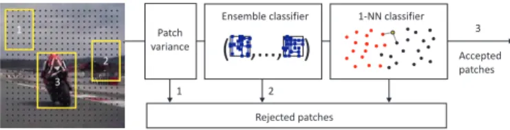
Ensemble classifier 1-NN classifier Patch variance Rejected patches Accepted patches

( ,..., )

Fig. 9. Block diagram of the object detector.

5.3 Object detector

The detector scans the input image by a scanning-window and for each patch decides about presence or absence of the object.

Scanning-window grid.We generate all possible scales and

shifts of an initial bounding box with the following parameters: scales step = 1.2, horizontal step = 10% of width, vertical step = 10% of height, minimal bounding box size = 20 pixels. This setting produces around 50k bounding boxes for a QVGA image (240x320), the exact number depends on the aspect ratio of the initial bounding box.

Cascaded classifier. As the number of bounding boxes

to be evaluated is large, the classification of every single patch has to be very efficient. A straightforward approach of directly evaluating the NN classifier is problematic as it involves evaluation of the Relative similarity (i.e. search for two nearest neighbours). As illustrated in figure 9, we structure the classifier into three stages: (i) patch variance, (ii) ensemble classifier, and (iii) nearest neighbor. Each stage either rejects the patch in question or passes it to the next stage. In our previous work [59] we used only the first two stages. Later on, we observed that the performance improves if the third stage is added. Templates allowed us to better estimate the reliability of the detection.

5.3.1 Patch variance

Patch variance is the first stage of our cascade. This stage rejects all patches, for which gray-value variance is smaller than 50% of variance of the patch that was selected for tracking. The stage exploits the fact that gray-value variance of a patch p can be expressed as _E(p2₎₋

E2(p), and that

the expected value _E(p) can be measured in constant time using integral images [35]. This stage typically rejects more than 50% of non-object patches (e.g. sky, street). The variance threshold restricts the maximal appearance change of the object. However, since the parameter is easily interpretable, it can be adjusted by a user for particular application. In all of our experiments we kept it constant.

5.3.2 Ensemble classifier

Ensemble classifier is the second stage of our detector. The in-put to the ensemble is an image patch that was not rejected by the variance filter. The ensemble consists ofnbase classifiers. Each base classifieriperforms a number ofpixel comparisons on the patch resulting in a binary codex, which indexes to an array of posteriors Pi(y|x), wherey∈ {0,1}. The posteriors of individual base classifiers are averaged and the ensemble classifies the patch as the object if the average posterior is larger than 50%. 1 0 0 0 1 1 0 1 1 1

pixel comparisons binary code input image + bounding box

blur measure

blurred image

output

Fig. 10. Conversion of a patch to a binary code.

Pixel comparisons.Every base classifier is based on a set

of pixel comparisons. Similarly as in [60], [61], [62], the pixel comparisons are generated offline at random and stay fixed in run-time. First, the image is convolved with a Gaussian kernel with standard deviation of 3 pixels to increase the robustness to shift and image noise. Next, the predefined set of pixel comparison is stretched to the patch. Each comparison returns 0 or 1 and these measurements are concatenated intox.

Generating pixel comparisons. The vital element of

en-semble classifiers is the independence of the base classi-fiers [63]. The independence of the classiclassi-fiers is in our case enforced by generating different pixel comparisons for each base classifier. First, we discretize the space of pixel locations within a normalized patch and generateallpossible horizontal and vertical pixel comparisons. Next, we permutate the com-parisons and split them into the base classifiers. As a result, every classifier is guaranteed to be based on a different set of features and all the features together uniformly cover the entire patch. This is in contrast to standard approaches [60], [61], [62], where every pixel comparison is generated independent of other pixel comparisons.

Posterior probabilities.Every base classifierimaintains a

distribution of posterior probabilitiesPi(y|x). The distribution has 2d _{entries, where d is the number of pixel comparisons.} We use 13 comparison, which gives 8192 possible codes that index to the posterior probability. The probability is estimated as Pi(y|x) = _#p#_+#p _n, where #p and #n correspond to number of positive and negative patches, respectively, that were assigned the same binary code.

Initialization and update. In the initialization stage, all

base posterior probabilities are set to zero, i.e. vote for negative class. During run-time the ensemble classifier is updated as follows. The labeled example is classified by the ensemble and if the classification is incorrect, the corresponding #p and#nare updated which consequently updatesPi(y|x).

5.3.3 Nearest neighbor classifier

After filtering the patches by the variance filter and the ensem-ble classifier, we are typically left with several of bounding boxes that are not decided yet (≈50). Therefore, we can use the online model and classify the patch using a NN classifier. A patch is classified as the object if Sr_{(p, M)> θ}

NN, where

θNN = 0.6. This parameter has been set empirically and its

value is not critical. We observed that similar performance is achieved in the range (0.5-0.7). The positively classified patches represent the responses of the object detector. When the number of templates in NN classifier exceeds some thresh-old (given by memory), we use random forgetting of templates. We observed that the number of templates stabilizes around

several hundred which can be easily stored in memory.

5.4 Tracker

The tracking component of TLD is based on Median-Flow tracker [64] extended with failure detection. Median-Flow tracker represents the object by a bounding box and estimates its motion between consecutive frames. Internally, the tracker estimates displacements of a number of points within the object’s bounding box, estimates their reliability, and votes with 50% of the most reliable displacements for the motion of the bounding box using median. We use a grid of10×10points and estimate their motion using pyramidal Lucas-Kanade tracker [65]. Lucas-Kanade uses 2 levels of the pyramid and represents the points by 10×10patches.

Failure detection.Median-Flow [64] tracker assumes

visi-bility of the object and therefore inevitably fails if the object gets fully occluded or moves out of the camera view. To identify these situations we use the following strategy. Letdi denote the displacement of a single point of the Median-Flow tracker and dm be the median displacement. A residual of a single displacement is then defined as |di−dm|. A failure of the tracker is declared if median|di−dm|>10 pixels. This strategy is able to reliably identify failures caused by fast motion or fast occlusion of the object of interest. In that case, the individual displacement become scattered around the image and the residual rapidly increases (the threshold of 10 pixels is not critical). If the failure is detected, the tracker does not return any bounding box.

5.5 Integrator

Integrator combines the bounding box of the tracker and the bounding boxes of the detector into a single bounding box output by TLD. TIf neither the tracker not the detector output a bounding box, the object is declared as not visible. Other-wise the integrator outputs the maximally confident bounding box, measured using Conservative similarity Sc_{. The tracker} and detector have identical priorities, however they represent fundamentally different estimates of the object state. While the detector localizes already known templates, the tracker localizes potentially new templates and thus can bring new data for detector.

5.6 Learning component

The task of the learning component is to initialize the object detector in the first frame and update the detector in run-time using the P-expert and the N-expert. An alternative explanation of the experts, called growing and pruning, can be found in [66].

5.6.1 Initialization

In the first frame, the learning component trains the initial detector using labeled examples generated as follows. The positive training examples are synthesized from the initial bounding box. First we select 10 bounding boxes on the scanning grid that are closest to the initial bounding box. For each of the bounding box, we generate 20 warped versions

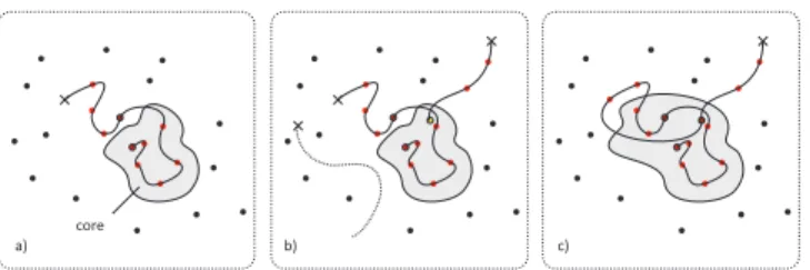
Fig. 11. Illustration of P-expert: a) object model and thecore in feature space (gray blob), b) unreliable (dotted) and reliable (thick) trajectory , c) the object model and the core after the update. Red dots are positive examples, black dots are negative, cross denotes end of a trajectory.

by geometric transformations (shift±1%, scale change±1%, in-plane rotation ±10◦_{) and add them with Gaussian noise}

(σ= 5) on pixels. The result is 200 synthetic positive patches. Negative patches are collected from the surrounding of the initializing bounding box, no synthetic negative examples are generated. If the application requires fast initialization, we sub-sample the generated training examples. The labeled training patches are then used to update the object model as discussed in subsection 5.2 and the ensemble classifier as discussed in subsection 5.3. After the initialization the object detector is ready for run-time and to be updated by a pair of P-N experts.

5.6.2 P-expert

The goal of P-expert is to discover new appearances of the object and thus increase generalization of the object detector. Section 4.4 suggested that the P-expert can exploit the fact that the object moves on a trajectory and add positive examples extracted from such a trajectory. However, in the TLD system, the object trajectory is generated by a combination of a tracker, detector and the integrator. This combined process traces a discontinuous trajectory, which is not correct all the time. The challenge of the P-expert is to identify reliable parts of the trajectory and use it to generate positive training examples.

To identify the reliable parts of the trajectory, the P-expert relies on an object model M. See figure 11 for reference. Consider an object model represented as colored points in a feature space. Positive examples are represented by red dots connected by a directed curve suggesting their order, negative examples are black. Using the conservative similaritySc_{, one} can define a subset in the feature space, where Sc _{is larger} than a threshold. We refer to this subset as the core of the object model. Note that the core is not a static structure, but it grows as new examples are coming to the model. However, the growth is slower than the entire model.

P-expert identifies the reliable parts of the trajectory as follows. The trajectory becomes reliable as soon as it enters the core and remain reliable until is re-initialized or the tracker identifies its own failure. Figure 11 (b) illustrates the reliable and non-reliable trajectory in feature space. And figure 11 (c) shows how the core changes after accepting new positive examples from reliable trajectory.

In every frame, the P-expert outputs a decision about the reliability of the current location (P-expert is an online pro-cess). If the current location is reliable, the P-expert generates

a set of positive examples that update the object model and the ensemble classifier. We select 10 bounding boxes on the scanning grid that are closest to the current bounding box. For each of the bounding box, we generate 10 warped versions by geometric transformations (shift±1%, scale change±1%, in-plane rotation ±5◦_{) and add them with Gaussian noise}

(σ = 5). The result is 100 synthetic positive examples for ensemble classifier.

5.6.3 N-expert

N-expert generates negative training examples. Its goal is to discover clutter in the background against which the detector should discriminate. The key assumption of the N-expert is that the object can occupy at most one location in the image. Therefore, if the object location is known, the surrounding of the location is labeled as negative. The N-expert is applied at the same time as P-expert, i.e. if the trajectory is reliable. In that case, patches that are far from current bounding box (overlap <0.2) are all labeled as negative. For the update of the object detector and the ensemble classifier, we consider only those patches that were not rejected neither by the variance filter nor the ensemble classifier.

6

Q

This section reports on a set of quantitative experiments comparing the TLD with relevant algorithms. The first two experiments (section 6.1, section 6.2) evaluate our system on benchmark sequences that are commonly used in the litera-ture. In both of these experiments, a saturated performance is achieved. Section 6.3 therefore introduces a new, more challenging dataset. Using this dataset, section 6.4 focuses on evaluation of the learning component of TLD. Finally, section 6.5 evaluates the whole system.

Every experiment in this section adopts the following eval-uation protocol. A tracker is initialized in the first frame of a sequence and tracks the object of interest up to the end. The produced trajectory is then compared to ground truth using a number of measures specified in the particular experiment.

6.1 Comparison 1: CoGD

TLD was compared with results reported in [33] which re-ports on performance of 5 trackers (Iterative Visual Track-ing (IVT) [22], Online Discriminative Features (ODV) [27], Ensemble Tracking (ET) [28], Multiple Instance Learning (MIL) [30], and Co-trained Generative-Discriminative track-ing (CoGD) [33]) on 6 sequences. The sequences include full occlusions and disappearance of the object. CoGD [33] dominated on these sequences as it enabled re-detection of the object. As in [33], the performance was accessed using the Number of successfully tracked frames,i.e. the number of frames where overlap with a ground truth bounding box is larger than 50%. Frames where the object was occluded were not counted. For instance, for a sequence of 100 frames with 20 occluded frames, the maximal possible score is 80.

Table 1 shows the results. TLD achieved the maximal possible score in the sequences and matched the performance of CoGD [33]. It was reported in [33] that CoGD runs at

TABLE 1

Number of successfully tracked frames – TLD in comparison to results reported in [33]. Sequence Frames Occ. IVT ODF ET MIL CoGD TLD

[22] [27] [28] [30] [33] David *761 0 17 - 94 135 759 761 Jumping 313 0 75 313 44 313 313 313 Pedestrian 1 140 0 11 6 22 101 140 140 Pedestrian 2 338 93 33 8 118 37 240 240 Pedestrian 3 184 30 50 5 53 49 154 154 Car 945 143 163 - 10 45 802 802 TABLE 2

Recall – TLD1.0 in comparison to results reported in [67]. Bold font means the best score.

Sequence Frames OB ORF FT MIL Prost TLD

[29] [68] [20] [30] [67] Girl 452 24.0 - 70.0 70.0 89.0 93.1 David 502 23.0 - 47.0 70.0 80.0 100.0 Sylvester 1344 51.0 - 74.0 74.0 73.0 97.4 Face occlusion 1 858 35.0 - 100.0 93.0 100.0 98.9 Face occlusion 2 812 75.0 - 48.0 96.0 82.0 96.9 Tiger 354 38.0 - 20.0 77.0 79.0 88.7 Board 698 - 10.0 67.9 67.9 75.0 87.1 Box 1161 - 28.3 61.4 24.5 91.4 91.8 Lemming 1336 - 17.2 54.9 83.6 70.5 85.8 Liquor 1741 - 53.6 79.9 20.6 83.7 91.7 Mean - 42.2 27.3 58.1 64.8 80.4 92.5

2 frames per second, and requires several frames (typically 6) for initialization. In contrast, TLD requires just a single frame and runs at 20 frames per second. This experiment demonstrates that neither the generative trackers (IVT [22]), nor the discriminative trackers (ODF [27], ET [28], MIL [30]) are able to handle full occlusions or disappearance of the object. CoGD will be evaluated in detail in section 6.5.

6.2 Comparison 2: Prost

TLD was compared with the results reported in [67] which reports on performance of 5 algorithms (Online Boosting (OB) [29], Online Random Forrest (ORF) [68], Fragment-baset Tracker (FT) [20], MIL [30] and Prost [67]) on 10 benchmark sequences. The sequences include partial occlu-sions and pose changes. The performance was reported using two measures: (i)Recall- number of true positives divided by the length of the sequence (true positive is considered if the overlap with ground truth is >50%), and (ii)Average local-ization Error - average distance between center of predicted and ground truth bounding box. TLD estimates scale of an object. However, the algorithms compared in this experiment perform tracking in single scale only. In order to make a fair comparison, the scale estimation was not used.

Table 2 shows the performance measured by Recall. TLD scored best in 9/10 outperforming by more than 12% the second best (Prost [67]). Table 2 shows the performance measured by Average localization error. TLD scored best in 7/10 being 1.6 times more accurate than the second best.

6.3 TLD dataset

The experiments 6.1 and 6.2 show that TLD performs well on benchmark sequences. We consider these sequences as saturated and therefore introduce new, more challenging data

TABLE 3

Average localization error – TLD in comparison to results reported in [67]. Bold means best.

Sequence Frames OB ORF FT MIL Prost TLD

[29] [68] [20] [30] [67] Girl 452 43.3 - 26.5 31.6 19.0 18.1 David 502 51.0 - 46.0 15.6 15.3 4.0 Sylvester 1344 32.9 - 11.2 9.4 10.6 5.9 Face occlusion 1 858 49.0 - 6.5 18.4 7.0 15.4 Face occlusion 2 812 19.6 - 45.1 14.3 17.2 12.6 Tiger 354 17.9 - 39.6 8.4 7.2 6.4 Board 698 - 154.5 154.5 51.2 37.0 10.9 Box 1161 - 145.4 145.4 104.5 12.1 17.4 Lemming 1336 - 166.3 166.3 14.9 25.4 16.4 Liquor 1741 - 67.3 67.3 165.1 21.6 6.5 Mean - 32.9 133.4 78.0 46.1 18.4 10.9 TABLE 4 TLD dataset

Name Frames Mov. Partial Full Pose Illum. Scale Similar camera occ. occ. change change change objects 1. David 761 yes yes no yes yes yes no 2. Jumping 313 yes no no no no no no 3. Pedestrian 1 140 yes no no no no no no 4. Pedestrian 2 338 yes yes yes no no no yes 5. Pedestrian 3 184 yes yes yes no no no yes 6. Car 945 yes yes yes no no no yes 7. Motocross 2665 yes yes yes yes yes yes yes 8. Volkswagen 8576 yes yes yes yes yes yes yes 9. Carchase 9928 yes yes yes yes yes yes yes 10. Panda 3000 yes yes yes yes yes yes no

set. We started from the 6 sequences used in experiment 6.1 and collected 4 additional sequences: Motocross, Volkswagen, Carchase and Panda. The new sequences are long and contain all the challenges typical for long-term tracking. Table 4 lists the properties of the sequences and figure 12 shows corre-sponding snapshots. The sequences were manually annotated. More than 50% of occlusion or more than 90 degrees of out-of-plane rotation was annotated as ”not visible”.

The performance is evaluated using precision P, recall R and f-measureF.P is the number of true positives divided by number of all responses,Ris the number true positives divided by the number of object occurrences that should have been detected.F combines these two measures asF = 2P R/(P+

R). A detection was considered to be correct if its overlap with ground truth bounding box was larger than 50%.

6.4 Improvement of the object detector

This experiment quantitatively evaluates the learning com-ponent of the TLD system on the TLD dataset. For every sequence, we compare the Initial Detector (trained in the first frame) and the Final Detector (obtained after one pass through the training). Next, we measure the quality of the P-N experts (P+_{, R}+_{, P}−_,R−_{) in every iteration of the learning and report}

the average score.

Table 5 shows the achieved results. The scores of the Initial Detector are shown in the 3rd column. Precision is above 79% high except for sequence 9, which contains a significant background clutter and objects similar to the target (cars). Recall is low for the majority of sequences except for sequence 5 where the recall is 73%. High recall indicates that the appearance of the object does not vary significantly and training the Initial Detector is sufficient.

The scores of the Final Detector are displayed in the 4th column. Recall of the detector was significantly increased with little drop of precision. In sequence 9, even the precision was increased from 36% to 90%, which shows that the false pos-itives of the Initial Detector were identified by N-experts and corrected. Most significant increase of the performance is for sequences 7-10 which are the most challenging of the whole set. The Initial Detector fails here but for the Final Detector the f-measure in the range of 25-83%. This demonstrates the improvement of the detector using P-N learning.

The last three columns of Table 5 report the performance of P-N experts. Both experts have precision higher than 60% except for sequence 10 which has P-precision just 31%. Recall of the experts is in the range of 2-78%. The last column shows the corresponding eigenvalues of matrix M. Notice that all eigenvalues are smaller than one. This demonstrates that the proposed experts work across different scenarios. The larger these eigenvalues are, the less the P-N learning improves the performance. For example in sequence 10 one eigenvalue is 0.99 which reflects poor performance of the P-N experts. The target of this sequence is an animal which performs out-of-plane motion. Median-Flow tracker is not very reliable in this scenario, but still P-N learning exploits the information provided by the tracker and improves the detector.

6.5 Comparison 3: TLD dataset

This experiment evaluates the proposed system on the TLD dataset and compares it to five trackers: (1) OB [29], (2) SB [31], (3) BS [69], (4) MIL [30], and (5) CoGD [33]. Binaries for trackers (1-3) are available in the Internet1. Trackers (4,5) were kindly evaluated directly by their authors. Since this experiment compares various trackers for which the default initialization (defined by ground truth) might not be optimal, we allowed the initialization to be selected by the authors. For instance, when tracking a motorbike racer, some algorithms might perform better when tracking only a part of the racer. When comparing thus obtained trajectories to ground truth, we performed normalization (shift, aspect and scale correction) of the trajectory so that the first bounding box matched the ground truth, all remaining bounding boxes were normalized with the same parameters. The normalized trajectory was then directly compared to ground truth using overlap and true positive was considered if the overlap was larger than 25%. As we allowed different initialization, the earlier used threshold 50% was found to be too restrictive.

Sequences Motocross and Volkswagen were evaluated by the MIL tracker [30] only up to the frame 500 as the algorithm required loading all images into memory in advance. Since the algorithm failed during this period, the remaining frames were considered as failed.

Table 6 show the achieved performance evaluated by precision/recall/f-measure. The last row shows a weighted average performance (weighted by number of frames in the sequence). Considering the overall performance accessed by F-measure, TLD achieved the best performance of 81% signif-icantly outperforming the second best approach that achieved

TABLE 5

Performance analysis of P-N learning. The Initial Detector is trained on the first frame. The Final Detector is trained using the proposed P-N learning. The last three columns show internal statistics of the training process.

Sequence Frames Initial Detector Final Detector P-expert N-expert Eigenvalues

Precision / Recall / F-measure Precision / Recall / F-measure P+_{, R}+ _P−_{, R}− _λ

1, λ2 1. David 761 1.00 / 0.01 /0.02 1.00 / 0.32 /0.49 1.00 / 0.08 0.99 / 0.17 0.92 / 0.83 2. Jumping 313 1.00 / 0.01 /0.02 0.99 / 0.88 /0.93 0.86 / 0.24 0.98 / 0.30 0.70 / 0.77 3. Pedestrian 1 140 1.00 / 0.06 /0.12 1.00 / 0.12 /0.22 0.81 / 0.04 1.00 / 0.04 0.96 / 0.96 4. Pedestrian 2 338 1.00 / 0.02 /0.03 1.00 / 0.34 /0.51 1.00 / 0.25 1.00 / 0.24 0.76 / 0.75 5. Pedestrian 3 184 1.00 / 0.73 /0.84 0.97 / 0.93 /0.95 0.98 / 0.78 0.98 / 0.68 0.32 / 0.22 6. Car 945 1.00 / 0.04 /0.08 0.99 / 0.82 /0.90 1.00 / 0.52 1.00 / 0.46 0.48 / 0.54 7. Motocross 2665 1.00 / 0.00 /0.00 0.92 / 0.32 /0.47 0.96 / 0.19 0.84 / 0.08 0.92 / 0.81 8. Volkswagen 8576 1.00 / 0.00 /0.00 0.92 / 0.75 /0.83 0.70 / 0.23 0.99 / 0.09 0.91 / 0.77 9. Car Chase 9928 0.36 / 0.00 /0.00 0.90 / 0.42 /0.57 0.64 / 0.19 0.95 / 0.22 0.76 / 0.83 10. Panda 3000 0.79 / 0.01 /0.01 0.51 / 0.16 /0.25 0.31 / 0.02 0.96 / 0.19 0.81 / 0.99

1. David 2. Jumping 3. Pedestrian 1 4. Pedestrian 2 5. Pedestrian 3

6. Car 7. Motocross 8. Volkswagen 9. Car Chase 10. Panda

Fig. 12. Snapshots from the introduced TLD dataset.

22%, other approaches range between 13-15%. The sequences have been processed with identical parameters with exception for sequence Panda, where any positive example added to the model had been augmented with mirrored version.

C

In this paper, we studied the problem of tracking of an unknown object in a video stream, where the object changes appearance frequently moves in and out of the camera view. We designed a new framework that decomposes the tasks into three components: tracking, learning and detection. The learn-ing component was analyzed in detail. We have demonstrated that an object detector can be trained from a single example and an unlabeled video stream using the following strategy: (i) evaluate the detector, (ii) estimate its errors by a pair of experts, and (iii) update the classifier. Each expert is focused on identification of particular type of the classifier error and is allowed to make errors itself. The stability of the learning is achieved by designing experts that mutually compensate their errors. The theoretical contribution is the formalization of this process as a discrete dynamical system, which allowed us to specify conditions, under which the learning process guarantees improvement of the classifier. We demonstrated that the experts can exploit spatio-temporal relationships in the video. A real-time implementation of the framework has

been described in detail. And an extensive set of experiments was performed. Superiority of our approach with respect to the closest competitors was clearly demonstrated. The code of the algorithm as well as the TLD dataset has been made available online2.

L

F

W

There are a number of challenges that have to be addressed in order to get more reliable and general system based on TLD. For instance, TLD does not perform well in case of full out-of-plane rotation. In that case the, the Median-Flow tracker drifts away from the target and can be re-initialized only if the object reappears with appearance seen/learned before. Current implementation of TLD trains only the detector and the tracker stay fixed. As a result the tracker makes always the same errors. An interesting extension would be to train also the tracking component. TLD currently tracks a single object. Multi-target tracking opens interesting questions how to jointly train the models and share features in order to scale. Current version does not perform well for articulated objects such as pedestrians. In case of restricted scenarios, e.g. static camera, an interesting extension of TLD would be to include background subtraction in order to improve the tracking capabilities.

Sequence Frames OB [29] SB [31] BS [69] MIL [30] CoGD [33] TLD 1. David 761 0.41 / 0.29 / 0.34 0.35 / 0.35 / 0.35 0.32 / 0.24 / 0.28 0.15 / 0.15 / 0.15 1.00 / 1.00 / 1.00 1.00 / 1.00 / 1.00 2. Jumping 313 0.47 / 0.05 / 0.09 0.25 / 0.13 / 0.17 0.17 / 0.14 / 0.15 1.00 / 1.00 / 1.00 1.00 / 0.99 / 1.00 1.00 / 1.00 / 1.00 3. Pedestrian 1 140 0.61 / 0.14 / 0.23 0.48 / 0.33 / 0.39 0.29 / 0.10 / 0.15 0.69 / 0.69 / 0.69 1.00 / 1.00 / 1.00 1.00 / 1.00 / 1.00 4. Pedestrian 2 338 0.77 / 0.12 / 0.21 0.85 / 0.71 / 0.77 1.00 / 0.02 / 0.04 0.10 / 0.12 / 0.11 0.72 / 0.92 / 0.81 0.89 / 0.92 / 0.91 5. Pedestrian 3 184 1.00 / 0.33 / 0.49 0.41 / 0.33 / 0.36 0.92 / 0.46 / 0.62 0.69 / 0.81 / 0.75 0.85 / 1.00 / 0.92 0.99 / 1.00 / 0.99 6. Car 945 0.94 / 0.59 / 0.73 1.00 / 0.67 / 0.80 0.99 / 0.56 / 0.72 0.23 / 0.25 / 0.24 0.95 / 0.96 / 0.96 0.92 / 0.97 / 0.94 7. Motocross 2665 0.33 / 0.00 / 0.01 0.13 / 0.03 / 0.05 0.14 / 0.00 / 0.00 0.05 / 0.02 / 0.03 0.93 / 0.30 / 0.45 0.89 / 0.77 / 0.83 8. Volkswagen 8576 0.39 / 0.02 / 0.04 0.04 / 0.04 / 0.04 0.02 / 0.01 / 0.01 0.42 / 0.04 / 0.07 0.79 / 0.06 / 0.11 0.80 / 0.96 / 0.87 9. Carchase 9928 0.79 / 0.03 / 0.06 0.80 / 0.04 / 0.09 0.52 / 0.12 / 0.19 0.62 / 0.04 / 0.07 0.95 / 0.04 / 0.08 0.86 / 0.70 / 0.77 10. Panda 3000 0.95 / 0.35 / 0.51 1.00 / 0.17 / 0.29 0.99 / 0.17 / 0.30 0.36 / 0.40 / 0.38 0.12 / 0.12 / 0.12 0.58 / 0.63 / 0.60 mean 26850 0.62 / 0.09 / 0.13 0.50 / 0.10 / 0.14 0.39 / 0.10 / 0.15 0.44 / 0.11 / 0.13 0.80 / 0.18 / 0.22 0.82 / 0.81 / 0.81 TABLE 6

Performance evaluation on TLD dataset measured by Precision/Recall/F-measure. Bold numbers indicate the best score. TLD1.0 scored best in 9/10 sequences.

A

The research was supported by the UK EPSRC EP/F0034 20/1 and BBC R&D grants (KM and ZK) and by EC project FP7-ICT-270138 Darwin and Czech Science Foundation project GACR P103/10/1585 (JM).

R

[1] A. Blum and T. Mitchell, “Combining labeled and unlabeled data with co-training,” Conference on Computational Learning Theory, p. 100, 1998.

[2] B. D. Lucas and T. Kanade, “An iterative image registration technique with an application to stereo vision,”International Joint Conference on Artificial Intelligence, vol. 81, pp. 674–679, 1981.

[3] J. Shi and C. Tomasi, “Good features to track,”Conference on Computer Vision and Pattern Recognition, 1994.

[4] P. Sand and S. Teller, “Particle video: Long-range motion estimation using point trajectories,” International Journal of Computer Vision, vol. 80, no. 1, pp. 72–91, 2008.

[5] L. Wang, W. Hu, and T. Tan, “Recent developments in human motion analysis,”Pattern Recognition, vol. 36, no. 3, pp. 585–601, 2003. [6] D. Ramanan, D. A. Forsyth, and A. Zisserman, “Tracking people by

learning their appearance,”IEEE Transactions on Pattern Analysis and Machine Intelligence, pp. 65–81, 2007.

[7] P. Buehler, M. Everingham, D. P. Huttenlocher, and A. Zisserman, “Long term arm and hand tracking for continuous sign language TV broadcasts,”British Machine Vision Conference, 2008.

[8] S. Birchfield, “Elliptical head tracking using intensity gradients and color histograms,”Conference on Computer Vision and Pattern Recognition, 1998.

[9] M. Isard and A. Blake, “CONDENSATION - Conditional Density Propagation for Visual Tracking,” International Journal of Computer Vision, vol. 29, no. 1, pp. 5–28, 1998.

[10] C. Bibby and I. Reid, “Robust real-time visual tracking using pixel-wise posteriors,”European Conference on Computer Vision, 2008. [11] C. Bibby and I. Reid, “Real-time Tracking of Multiple Occluding

Objects using Level Sets,”Computer Vision and Pattern Recognition, 2010.

[12] B. K. P. Horn and B. G. Schunck, “Determining optical flow,”Artificial intelligence, vol. 17, no. 1-3, pp. 185–203, 1981.

[13] T. Brox, A. Bruhn, N. Papenberg, and J. Weickert, “High accuracy optical flow estimation based on a theory for warping,” European Conference on Computer Vision, pp. 25–36, 2004.

[14] J. L. Barron, D. J. Fleet, and S. S. Beauchemin, “Performance of Optical Flow Techniques,”International Journal of Computer Vision, vol. 12, no. 1, pp. 43–77, 1994.

[15] D. Comaniciu, V. Ramesh, and P. Meer, “Kernel-Based Object Track-ing,”IEEE Transactions on Pattern Analysis and Machine Intelligence, vol. 25, no. 5, pp. 564–577, 2003.

[16] I. Matthews, T. Ishikawa, and S. Baker, “The Template Update Prob-lem,”IEEE Transactions on Pattern Analysis and Machine Intelligence, vol. 26, no. 6, pp. 810–815, 2004.

[17] N. Dowson and R. Bowden, “Simultaneous Modeling and Tracking (SMAT) of Feature Sets,”Conference on Computer Vision and Pattern Recognition, 2005.

[18] A. Rahimi, L. P. Morency, and T. Darrell, “Reducing drift in differential tracking,”Computer Vision and Image Understanding, vol. 109, no. 2, pp. 97–111, 2008.

[19] A. D. Jepson, D. J. Fleet, and T. F. El-Maraghi, “Robust Online Appearance Models for Visual Tracking,”IEEE Transactions on Pattern Analysis and Machine Intelligence, pp. 1296–1311, 2003.

[20] A. Adam, E. Rivlin, and I. Shimshoni, “Robust Fragments-based Track-ing usTrack-ing the Integral Histogram,”Conference on Computer Vision and Pattern Recognition, pp. 798–805, 2006.

[21] M. J. Black and A. D. Jepson, “Eigentracking: Robust matching and tracking of articulated objects using a view-based representation,” Inter-national Journal of Computer Vision, vol. 26, no. 1, pp. 63–84, 1998. [22] D. Ross, J. Lim, R. Lin, and M. Yang, “Incremental Learning for Robust

Visual Tracking,” International Journal of Computer Vision, vol. 77, pp. 125–141, Aug. 2007.

[23] J. Kwon and K. M. Lee, “Visual Tracking Decomposition,”Conference on Computer Vision and Pattern Recognition, 2010.

[24] M. Yang, Y. Wu, and G. Hua, “Context-aware visual tracking.,”IEEE transactions on pattern analysis and machine intelligence, vol. 31, pp. 1195–209, July 2009.

[25] H. Grabner, J. Matas, L. Van Gool, and P. Cattin, “Tracking the Invisible: Learning Where the Object Might be,”Conference on Computer Vision and Pattern Recognition, 2010.

[26] S. Avidan, “Support Vector Tracking,”IEEE Transactions on Pattern Analysis and Machine Intelligence, pp. 1064–1072, 2004.

[27] R. Collins, Y. Liu, and M. Leordeanu, “Online Selection of Discrimi-native Tracking Features,”IEEE Transactions on Pattern Analysis and Machine Intelligence, vol. 27, no. 10, pp. 1631–1643, 2005.

[28] S. Avidan, “Ensemble Tracking,”IEEE Transactions on Pattern Analysis and Machine Intelligence, vol. 29, no. 2, pp. 261–271, 2007. [29] H. Grabner and H. Bischof, “On-line boosting and vision,”Conference

on Computer Vision and Pattern Recognition, 2006.

[30] B. Babenko, M.-H. Yang, and S. Belongie, “Visual Tracking with Online Multiple Instance Learning,” Conference on Computer Vision and Pattern Recognition, 2009.

[31] H. Grabner, C. Leistner, and H. Bischof, “Semi-Supervised On-line Boosting for Robust Tracking,” European Conference on Computer Vision, 2008.

[32] F. Tang, S. Brennan, Q. Zhao, H. Tao, and U. C. Santa Cruz, “Co-tracking using semi-supervised support vector machines,”International Conference on Computer Vision, pp. 1–8, 2007.

[33] Q. Yu, T. B. Dinh, and G. Medioni, “Online tracking and reacquisi-tion using co-trained generative and discriminative trackers,”European Conference on Computer Vision, 2008.

[34] D. G. Lowe, “Distinctive image features from scale-invariant keypoints,”

International Journal of Computer Vision, vol. 60, no. 2, pp. 91–110, 2004.

[35] P. Viola and M. Jones, “Rapid object detection using a boosted cas-cade of simple features,” Conference on Computer Vision and Pattern Recognition, 2001.

[36] V. Lepetit, P. Lagger, and P. Fua, “Randomized trees for real-time keypoint recognition,” Conference on Computer Vision and Pattern Recognition, 2005.

[37] L. Vacchetti, V. Lepetit, and P. Fua, “Stable real-time 3d tracking using online and offline information,”IEEE Transactions on Pattern Analysis and Machine Intelligence, vol. 26, no. 10, p. 1385, 2004.