An Empirical Analysis of the Buoyancy and Elasticity of Tax in Nigeria

An Empirical Analysis of the Buoyancy and Elasticity of Tax in

Nigeria

Ikpeze N. I. David-Wayas, O. M. Musa, O. D. University of Nigeria, Nsukka, Nigeria

Abstract

Many countries in the world have greatly sponsored their government expenditures with the aid of tax revenue, and owe their developments to this internally generated revenue. The rate of increase depends on the elasticity and buoyancy of tax and it is on this premise that, this study investigated the elasticity and buoyancy of tax in an attempt to ascertain its flexibility and hence the possibility of increasing the tax base in Nigeria. The results of the study therefore suggest that aggregate revenue is relatively elastic and significantly buoyant according to the 2004 tax reforms. And the results of the four major taxes tested showed that only PPT was found to be relatively elastic while VAT, CED and CID were relatively inelastic. However the results further suggest that, while VAT and CIT are not significantly buoyant according to the 2004 tax reforms, PPT and CED are significantly buoyant. Finally, the study used the 2005 structural break to establish that aggregate tax revenue dropped significantly after the boom period. The study therefore concludes that tax in Nigeria is relatively flexible with respect to growth and therefore more could be done to increase it.

Keywords: Tax, tax reform, elasticity, buoyancy, Nigeria.

Background to the Study

Tax is a major source of government revenue all over the world. Governments use tax proceeds to render their traditional functions such as the provision of public goods, maintenance of law and order, defense against external aggression, regulation of trade and business to ensure social and economic maintenance (Azubike, 2009). The economic effects of tax include micro effects on the distribution of income and efficiency of resources use as well as macro effect on the level of capacity output, employment, prices and growth (Musgrave and Musgrave, 2004).

Among all the sources of revenue to government, taxation is the most important one. Owing to the inherent power of government to impose taxes, the government is assured at all times of its tax revenue no matter the circumstances. With modifications as a result of different manifestos of opposing political parties, the government’s ability to impose tax is unlimited. It is in this light of the significance of this source of government revenue that its assessment, effectiveness and collectivity are paramount for optimum benefit (Effiok, 2006).

The Nigerian tax system is lopsided, and dominated by oil revenue. The most veritable tax handles are under the control of the federal government while the lower tiers are responsible for the less strong ones—the federal government taxes corporate bodies while state and local governments’ tax individuals. A major element contributing to this development was the prolonged military rule that had ignored constitutional provision. During the early stage of the country’s economy, revenues were largely derived from primary products. Between 1960 and the early 1970s, revenue from agricultural products dominated, while revenue from other sources was considered as residual. Since the oil boom of 1973/4 to date, however, oil has dominated Nigeria’s revenue profile, thus, indicating that traditional tax revenue has not assumed a strong role in the country’s management of fiscal policy. Instead of transforming or diversifying the existing revenue base, fiscal management has merely transited from one primary product-based economy to another, making the economy susceptible to fluctuations of the international oil market.

The need to address this problem led to several taxes policy reforms. The tax policy reviews of 1991 and 2003, as well as the yearly amendments given in the annual budget, were geared towards addressing this issue. But not much has been achieved. Perhaps to understand the importance of tax policy reforms, one needs to appreciate the urgency for such reforms. Why the need for tax policy reforms in Nigeria? First, there is a compelling need to diversify the revenue portfolio for the country in order to safeguard against the volatility of crude oil prices and to promote fiscal sustainability and economic viability at lower tiers of government. Second, Nigeria operates on a cash budget system, where proposals for expenditure are always anchored to revenue projections. This facilitates determining the optimal tax rate for a given level of expenditure. Thus accuracy in revenue projection is vital for devising an appropriate framework for sustainable fiscal management, and this can be realized only if reforms are undertaken on existing tax policies in order to achieve some improvement.

Thirdly, the study groups on the review of the Nigerian tax system in 1991 and 2003 highlighted the need to increase tax revenue and reduce expenditure as the major fiscal issues to be addressed. As such, the primary objective of the committees was to optimize revenue from various sources within the country. Finally, the necessity to improve the tax notification procedure was underscored in order to facilitate effective evaluation of the performance of the Nigerian tax system and to promote adequate planning and implementation. The

quality of management associated with regular and a result-oriented tax reform has a significant bearing on the overall macroeconomic performance and the distribution of resources between public and private sectors as well as within the public sector.

Besides, Wagner’s law stipulates that public expenditure is a natural consequence of economic growth (Demirbas, 1999). The magnitude of government surplus or deficit is probably the single most important statistic measuring the impact of government fiscal policy on an economy (Siegel, 1979). Many developing countries including Nigeria in their attempt to increase growth have increased public expenditure but have not been able to match this increase with revenue mobilization through taxation and this has resulted in huge fiscal deficit. In the case of Nigeria, tax mobilization as a source for financing development activities has been a difficult issue primarily because of various forms of resistance such as evasion, avoidance and corrupt practices attending to it. These activities are considered as sabotaging the economy and are readily presented as reasons for the underdevelopment of the country (Adegbie and Fakile, 2011). Again, the Nigerian tax system has been weak in its revenue mobilization due to inadequate data on the tax base and heavy reliance on oil revenue. With the volatility in oil prices and excruciating impacts of the recent global financial crises, taxation deserves more attention now than ever in Nigeria (Adeleke, 2011).

An accurate estimate of the optimal level of expenditure requires knowledge of the buoyancy-total response of tax revenue to changes in national income and discretionary changes in tax policy over time; and tax elasticity- automatic response of tax revenue to GDP changes less the discretionary changes. It assists in identifying a sustainable revenue profile for the country and also helps in determining appropriate modifications to the existing tax structure and rates as well as areas for improving tax administration.

Statement of the Problem

Fiscal deficit has become a recurring feature of public sector financing all over the world. Its widespread use is partly influenced by the desire of various governments to respond positively to the ever-increasing demands of the populace and to enhance accelerated economic growth and development (Ariyo, 1993). This tendency toward deficit financing is more pronounced in developing countries where the populace looks to the government for the satisfaction of most needs. However, the rising magnitude of this deficit since 1980 in Nigeria is now of great concern. An appraisal of the budgetary process in Nigeria shows that annual expenditure proposals are always anchored on projected revenue, thus, the accuracy of revenue projection which requires the knowledge of buoyancy and elasticity of tax is a necessary condition for devising an appropriate framework for fiscal deficit management in Nigeria.

The federal government of Nigeria (FGN) commenced the implementation of a structural Adjustment programme (SAP) in 1986 that amounted to significant structural changes in the macroeconomic management framework for the country. One of the core objectives of the SAP is to enhance the degree of self-reliance within the economy. Of equal importance is the need to diversify the economy’s revenue base, in order to minimize the extent of dependence on oil as the major source of revenue. All these have potential implications for the yield of non-oil tax revenue sources. For example, one major consequence of SAP is the rekindled interest in export of cash crops such as cocoa. Ordinarily, this should have resulted in a significant upsurge in revenue from export duties, but as part of the reform, the FGN scrapped export duties as an element of the package of incentives meant to promote exports. There were significant downward revisions in tax rates and import tariffs as well. The corporate tax rate was reduced from 45% to 40% in 1987 in order to encourage re-investment activities by existing organizations and to encourage new investments. Similarly, import duties on certain categories of imports were reviewed. Among these was the elimination of duties on trucks and commercial vehicles to ease the transportation problem in the country. Also duty exemptions were granted on items required on some public projects. Generous tariff concessions were also allowed on machinery and raw materials that could not be sourced locally, at least not in the short run. Several policies having implications for the yield of specific tax sources were also initiated to mitigate the negative effect of SAP on the populace. The introduction of SAP generated several changes in tax-related policies, so that any growth in GDP during this period might not necessarily translate into higher tax yield. The determination of the buoyancy and elasticity of individual main taxes therefore becomes an empirical question.

However, before the above economic reform, the advent of the oil boom in the 1973/74 fiscal year encouraged over-reliance on oil revenue to the neglect of traditional revenue sources. As a result, some non-oil revenue sources were either abandoned or became of less concern to the government, hence, the need to assessing the optimal revenue derivable from these non-oil sources and to equally find out the changes that this major experience had brought about.

The motivation of this study however, is to ascertain the elastic nature of tax and its buoyancy with respect to tax reforms. Elasticity of tax in this study measures the proportion of change of tax, with respect to a unit change in economic growth. It is the interest of this study to analyze the elasticity of the aggregate tax and four of the major taxes. Also the need to improve non-oil proceeds has been on an increase over the years and so

many tax reforms have been made to boast tax revenue. This study therefore investigates to what extent the 2004 tax reform was buoyant to the tax base.

Based on this background the study seeks to answer the following research questions; 1. What is the tax buoyancy and elasticity of the total tax revenue in Nigeria?

2. What is the tax buoyancy and elasticity of the main taxes in Nigeria namely; Company Income Tax, Petroleum Profit Tax, Custom and Excise Duties and Value Added Tax (VAT)?

3. What are the major structural changes in the tax revenue before and after the oil- boom in Nigeria? The broad objective of this study is to analyze empirically the buoyancy and elasticity of tax system in Nigeria with respect to its efficiency in revenue mobilization in the attempt to address the unsustainable fiscal deficit challenge facing the country.

The specific objectives are:

1. Toascertain the tax buoyancy and elasticity of the Total Tax Revenue in Nigeria.

2. To ascertain the tax buoyancy and elasticity of the main taxes in Nigeria namely; Company Income Tax, Petroleum Profit Tax, Custom and Excise Duties and Value Added Tax (VAT).

3. To investigate the presence of structural change in tax revenue during and after the oil-boom in Nigeria. The hypothesis of the study is formally stated in its null form while the alternative is implied. Ho1: The total tax revenue in Nigeria is not significantly buoyant.

Ho2: Tax revenue of the main taxes in Nigeria with respect to GDP growth are not significantly buoyant.

Ho3: There is no significant structural change in tax revenue between the pre and post oil-boom era in Nigeria.

Significance of the Study

An accurate estimation of the optimal level of expenditure requires knowledge of the buoyancy and elasticity of the tax system. The study will help the government to know if they are keeping track on tax revenue mobilization with respect to GDP growth. Additionally, estimation of individual tax buoyancy and elasticity would help the policy makers especially the fiscal authorities to identify those taxes which are income elastic or otherwise and therefore aim at directing their efforts at the more elastic ones to raise overall tax revenue and making sure that the inelastic ones become elastic. Besides, the estimation of decomposed buoyancy into the pre and post oil- boom era helps to shed more light on the weaknesses and strengths of the system that existed before and what pertains today. This also helps the tax authorities in identifying issues that need improvement and restructuring in the Nigerian tax system.

Finally, to academicians, this work will serve as a reference point for further research and consequently add to the existing stock of literature in public sector Economics.

The scope of the study

This study investigates empirically the buoyancy and elasticity of the Nigerian tax system (that is, the efficiency of tax system in terms of its revenue mobilization capacity with respect to GDP) from 1980-2011 bearing in mind the effect of the 2004 major tax reform in Nigeria to determine the buoyancy as the tax base experienced changes. Four major taxes were considered namely; Company Income Tax, Petroleum Profit Tax, Custom and Excise Duties and Value Added Tax (VAT). It also incorporates the behavior of tax system before and after oil- boom in Nigeria. The core variable of interest are; National income, Government expenditure, External Grant, Non-Tax Revenue, Budget Deficit and Inflation as the control variable.

Conceptual Framework

Every country in the process of formulating its budget undertakes revenue projections. When the revenues turn out to be smaller than the budget expenditures, countries end up with deficit financing. Since underdeveloped countries have few possibilities for prolonged external financing of budget deficits, without causing too much disruption in the macroeconomic environment, each country must decide how best to increase its internal tax revenues to meet its expenditure needs. One way that countries raise additional revenue is by making discretionary tax measure changes. The best outcome expected from such changes is that the tax system will automatically yield corresponding tax revenues as income or GDP grows, on a sustainable basis.

Elasticity of Tax

Tax elasticity is the ratio of the percentage change in tax revenue to the percentage change in income or GDP, assuming that no discretionary changes have been made in the tax rate or tax base. It is defined as:

Where: ETY = Elasticity of tax revenue to income or GDP,

Mirambo (2001), Elasticity measures the responsiveness of tax revenue to changes in national income if the tax structure would have remained unchanged. To estimate elasticity of any tax system, revenue series have to be corrected for the effects of discretionary changes in tax policy.

Mansfield (1972) argues that automatic growth in tax revenue alone, abstracting from discretionary changes, is the elasticity of the tax. High tax elasticity, that is, a tax elasticity coefficient of one or more, is said to be particularly desirable since it allows growth in expenditure to be financed by raising tax revenue without recourse to the politically unpopular decision to raise tax rates.

Tsegaye (1993) says that a high elasticity may simply reflect the progressiveness of the tax structure, showing positive ratios of tax revenues to increases in income. A high elasticity (that is greater than unity) implies that the tax revenue increases faster than the income. This means if the tax is meant to maximize revenue, the government could rely on more elastic taxes which do not require frequent discretionary changes. It is therefore essential that the tax elasticity be equal to or exceeds unity to maximize revenue.

Tax Buoyancy

The buoyancy of tax measures the responsiveness of tax revenue to changes in income without controlling for the discretionary changes in tax policy. The discretionary changes are the changes which result in more tax revenue from the same tax base. The sources of such changes are changes in tax legislation or changes in the tax rate (Osoro 1993)

Jayasundera (1991) explains that the buoyancy of a tax system reflects the total response of tax revenue to changes in national income as well as effects of discretionary changes in tax policies over time. Matundu (1995) adds to the view of Jayasundera that a buoyancy coefficient which is greater than one would imply that for every one percent increase in GDP, tax revenue increases by more than one percent.

Tax Reforms in Nigeria

The Nigerian tax reform has experienced series of reforms since 1904 to date. The effects of the various reforms in the country is as follows: Introduction of income tax in Nigeria between 1904 and 1926; grant of autonomy to the Nigerian Inland Revenue in 1945; the Raisman Fiscal Commission of 1957; formation of the Inland Revenue Board in 1958; the promulgation of the petroleum profit tax ordinance No. 15 of 1959; the promulgation of Income Tax Management Act 1961; establishment of the Lagos State Inland Revenue Department; the promulgation of the companies Income Tax Act (CITA) 1979; establishment of the Federal Board of Internal Revenue Service between 1991 and 1992; and tax policy and administration reforms amendment 2001 and 2004. The government embarked upon the latest tax reform process by instituting study group on the Nigerian Tax System, consisting of individuals from business, academia, and the government to study the present tax laws and recommend the appropriate reform in general and their impact to the overall economy. As a result of the reform, nine (9) bills on tax reforms where approved by the Federal Executive Council for the consideration of the National Assembly and subsequently passed as Act. The Acts, are as enumerated as follows: Federal Inland Revenue Service Act 2004; companies Income Tax Act 2004; Petroleum Profit Tax Act 2004; Personal Income Tax Act 2004; Value Added Act 2004; Education Tax Act 2004; Customs, Excise Tariffs, etc (consolidation) Act 2004; National Sugar Development Act 2004; and National Automotive Council Act 2004.

The Chartered Institute of Taxation of Nigeria (CITN), established in 1982 and Chartered by Act No. 76 of 1992 to regulate tax practice and administration in the country, and to this extent a major stakeholder in the Nigerian tax system submitted a memorandum on the proposed 2004 amendment. Their memorandum objectives include: to strengthen the powers of the Accountant General of the federation to monitor the revenue being generated by ministries, extra-ministerial departments and parastatals; to enforce remittance of the revenues collected to the consolidated revenue fund or federation account; to strengthen the oversight functions of the National Assembly in monitoring the revenue generated by ministries, and others; to increase the penalty for under declaration of revenue generated from three to five years.

Personal Income Tax (Ammendment) Act 2011 ( Pitam)

An Act, Personal Income Tax (Amendment) Act, 2011 was enacted to amend the Personal Income Tax Act, Cap. P8. Laws of the Federation of Nigeria (LFN) 2004 and related matters. The Bill seeks to amend the provisions of the Principal Act, Personal Income Tax Act, Cap. P8. LFN 2004, by substituting the existing Sixth Schedule with the new Sixth Schedule. It was signed into law on 14 June 2011 but only announced during the budget presentation by the President on 13 December 2011.

Key Changes

The highlights of the New Personal Income Tax (Amendment) Act, 2011 are as follows:

· Gross income is defined to include benefits in kind, gratuities, superannuation and any other incomes derived solely by reason of employment.

· Principal place of residence to include places where branch offices and operational site of companies are situated.

· Operational sites are defined in the bill to include oil terminals, oil platforms, flow stations, construction sites, etc with a minimum of 50 workers.

· Any individual irrespective of status who works in more than one state for at least 20 days in at least 3 months of every assessment year will be liable to tax in such a state.

· Full tax exemption to be granted on interest from bonds issued by Federal, State and Local Governments and their Agencies, corporate entities and interest earned on short term securities.

· Interest for default in tax remittance to be charged at the prevailing minimum re-discount rate of the Central Bank of Nigeria on an annual basis.

· Individual tax clearance certificates (TCC) to be required for any change of ownership of vehicles and application for land title transfer or perfection.

· 1% bonus which was previously given to early filers of tax returns has been abolished.

· Amendment to Section 33 is a new insertion to introduce a presumptive tax regime to bring in those in the informal sector to the Tax Net. The section highlights the fact that “There will be a consolidated tax free allowance of N200, 000 or 1% of gross income whichever is higher plus 20% of the gross income, the balance of income shall be taxed as specified in the new graduated tax table.”

· Amendment to Section 37 is a new insertion to increase the Minimum Tax rate payable from 0.5% to 1% of gross income since the threshold has increased from N30,000 to N300,000 in conformity with the tax table in the schedule to the Bill.

· Section 52 introduces stiffer criminal penalties for non-compliance. Penalty for late filing of returns is now N500,000 for corporate bodies and N50,000 for individuals.

· Amendment to Section 73 is to create a refund mechanism. “Introduction of WHT refund mechanism. The excess WHT will be refunded within 90 days or granted as future tax credits”

· Section 80 New PAYE filing requirement: It is mandatory for employers of labour to file returns of their employees not later than 31 January of every year; showing all the emoluments paid to its employees in the preceding year.

· Tax officers to apply for a warrant from the High Court before levying any distress on a taxpayer.

· “itinerant worker”previously defined to mean an individual who works at any time during a year of assessment (other than as a member of the armed forces) for a daily wage or customarily earns his livelihood in more than one place in Nigeria and whose total income does not exceed N 600; to be modified as follows:

· “itinerant worker includes an individual irrespective of his status who works at any time in any state during a year of assessment (other than as a member of the armed forces) for wages, salaries or livelihood by working in more than one state for a minimum of twenty (20) days in at least three (3) month of every assessment year. The relevant tax authorities are empowered to collect taxes from itinerant worker.”

· Place of Residence for an itinerant worker has been amended thus: “in the case of an individual who works in the branch office or operational site of a company or other body corporate, the place at which the branch office or operation site is situated: Provided that operational site shall include Oil Terminals, Oil Platforms, Flow Stations, Factories, Quarries, Construction Site with a minimum of fifty (50) workers etc”.

Empirical Studies

Empirical literature exists on tax revenue and reforms in a sizeable number. However, this study narrows its focus on the buoyancy and elasticity of tax. Some of the research been carried out on buoyancy and elasticity of tax are reviewed in this section.

Osoro (1993) study on the revenue productivity of the tax system in Tanzania for the period 1969-1990 showed a low elasticity for the total tax system, as well as for individual taxes.

Ole (1975) estimated income elasticity of tax structure of Kenya for the period 1962-1972. Tax revenue was regressed on income without adjusting for the unusual observations. The results showed that the tax structure was income inelastic with an index of 0.81 for the period studied.

Choudhry (1979) estimated the elasticity of tax revenue of the United States, United Kingdom, Malaysia and Kenya. The overall elasticity were 1.04 and 1.24 for the United States and United Kingdom respectively. Malaysia and Kenya had slightly higher elasticity of 1.57 and 32 respectively. Estimation of the buoyancy revealed that in the United States and the United Kingdom, revenue reducing discretionary changes in income taxation contributed to the low buoyancy and elasticity, while in Malaysia and Kenya, revenue increasing DTMs contributed to the comparatively higher buoyancy and elasticity.

In the similar view, Mtatifikolo (1990); Njoroge (1993); Kusi (1998);Milambo (2001) and Graeser (2004), in their respective studies showed that generally, broad consumption taxes usually show elasticity slightly less and part of this can be explained by the specific nature of the individual economy.

run and buoyancy exceeded the elasticity, but in the short run the reverse was the case. They also observed an improvement in both buoyancy and elasticity over the reform period.

Milwood, T.T (2012) Studied the relationship between GDP growth and the growth in tax revenue as well as the responsiveness of taxes to fiscal policy in Jamaica. The study observed that discretionary tax measures have had an overall impact on growth in total revenue over the period. However, the automatic response of revenue to changes in the base was found to be less than unity.

Omorugi (1983) did a comprehensive assessment of the productivity of the Nigerian tax system. He evaluated the buoyancy of the tax system as defined by Sahota (1961) and Ghai (1966) for the period 1960 to 1979. He focused on both the indirect taxes such as import, export and excise duties, as well as direct taxes such as personal income tax (federally collected) and petroleum profit tax. He discovered a general satisfaction on the level of tax productivity in Nigeria during the period under review.

Ariyo (1997) in his study of the productivity of the Nigerian tax system improved upon the one done by Omrugi (1983) in the following respects. First, the study covered the period 1960-1990, and therefore updates the analysis. Second, the study captured the impact of the structural changes in macroeconomic management framework introduced since 1966. Third, Omoruyi (1983) disaggregated his analysis in terms of decades (1960-1967, 1970-1980, etc). His research findings were as follows: For the period covered by the study, there was an elasticity of 1.18 for government tax revenue relative to GDP. The non-oil component, however, had a lower elasticity coefficient of 0.94, while the performance of import duties (IMD) showed the same pattern. The cumulative effect of the oil boom PPT (petroleum profit tax) was reflected with an elasticity of 2.60 and 1.51 in relation to GDP. He also found out that company income tax was elastic with an elasticity coefficient of 1.21, which suggests an improved efficiency in tax collection from this source over the years.

Model Specifications

Estimation of Tax Elasticity and Buoyancy

This study captures elasticity and buoyancy based on their definitions as stated above. Tax elasticity is defined as “the ratio of the percentage change in tax revenue to the percentage change in income or GDP”, this therefore implies that tax elasticity is the coefficient of GDP/Income on tax revenue, both for individual taxes and for the total tax revenue. “In empirical works an elasticity is the estimated coefficient in a linear regression equation where both the dependent variable and the independent variable are in natural logs. Elasticity is a popular tool among empiricists because it is independent of units and thus simplifies data analysis” (Wikipedia 2013). The coefficient of the GDP describes elasticity and it is defined thus

Table 1: Types of elasticity and designations

Alternative Coefficient (E)

Perfectly Elastic E= ∞

Relatively Elastic (more than proportionate change) 1 < E < ∞

Unit Elastic (equal proportional change) E=1

Relatively Inelastic (Less than proportionate change) 0 < E< 1

Perfectly Inelastic E = 0

While Tax Buoyancy is defined as “a measurement of the responsiveness of tax revenue to changes in income without controlling for the discretionary changes in tax policy. The discretionary changes are the changes which result in more tax revenue from the same tax base. The sources of such changes are changes in tax legislation or changes in the tax rate” which suggests that the dummy variable for tax reforms of 2004 captures discretional changes in the tax base, hence the buoyancy.

Model Specification of the objectives of the study

In line with the major focus of this study which is to investigate the buoyancy and elasticity of tax system in Nigeria with respect to its efficiency in revenue mobilization vis-à-vis the changes in National Income (NI), thus, we assume aggregate revenue to be a homogenous function of NI. Putting this in a more sophisticated procedure where economic theory suggests equilibrium relationship among aggregate revenue and the national income; there are several forms of these equilibrium relations to hold using these variables, hence a motivation for a system of equations. Also in recognition of the deterministic trend (denoted with h) of fiscal policy instrument, we formulate the model for the estimation of objective 1, that is, the buoyancy and elasticity of tax estimate with respect to national income in the following standard regression technique equation;

t 10

+

11

+

12 13 14 15 16 17 1

....(1)

k

t t t t t t t t t

ARV

=

α

θ

Z

φ

NI

+

φ

GX

+

φ

NTR

+

φ

XG

+

φ

INF

+

ψ

D

+ +

h

ε

Where

ARV = Aggregate Tax Revenue NI = National Income (GDP) GX = Government Expenditure

NTR = Non-Tax Revenue XG = External Grant INF = Inflation rate

Dt = Dummy variable for tax reforms (where 0= 1980-2003 and 2004-2011)

Z = total base of tax k at time t;

θ = the elasticity of tax base with respect to national income

h = deterministic trend, since most fiscal policy instrument are trending;

ε = stochastic error terms.

Equation 1 estimates the buoyancy and elasticity of aggregate tax revenue with respect to national income. However, estimating the individual taxes revenue in terms of buoyancy and elasticity (as given in objective 2), we develop the following equations.

t 10

+

11 1 12 13 14 15 16 17 18 1

...(2)

k

t t t t t j t

PIT

=

α

φ

Z

−

+

φ

NI

+

φ

EP

+

φ

TW

+

φ

INF

+

φ

RER

+

φ

BD

+

φ

D

+

ε

t 20

+

21 1 22 25 26 27 2

...(3)

k t t t j t

CIT

=

α

φ

Z

₋

+

φ

NI

+

φ

INT

+

φ

CDB

+

φ

D

+

ε

t 30

+

31 1 32 33 35 36 37 3

...(4)

k t t t t j t

PPT

=

α

φ

Z

₋

+

φ

NI

+

φ

BD

+

φ

RER

+

φ

RCO

+

φ

D

+

ε

t 40

+

41 1 42 43 45 46 47 3

...(5)

k t t t t j t

ED

=

α

φ

Z

−

+

φ

NI

+

φ

BD

+

φ

RER

+

φ

TPR

+

φ

D

+

ε

t 50

+

51 1 52 53 54 55 56 5

...(6)

k t t t t t j t

CED

=

α

φ

Z

₋

+

φ

NI

+

φ

BD

+

φ

RER

+

φ

IMP

+

φ

D

+

ε

t 60

+

61 1 62 63 64 65 66 67 6

...(7)

k

t t t t t j t

VAT

=

α

φ

Z

−

+

φ

NI

+

φ

BD

+

φ

BOT

+

φ

INF

+

φ

CS

+

φ

D

+

ε

All equations (1 to 7) were linearized to ascertain the elasticity given that elasticity in regression coefficients are the estimated coefficients where both the dependent variable and the independent variable are in natural logs. Where

PIT = Personal Income Tax CIT = Company Income Tax PPT = Petroleum Profit tax ET = Education Tax

CED = Custom & excise Duties, and VAT = Value Added Tax

INF = Inflation rate BD = Budget deficit RER = Real exchange rate BOT = Balance of trade EP = Employed Population TW = Total Wage

CDB = Cost of doing Business RCO = Revenue from crude oil TPR = Total production revenue IMP = Import

CS = Company sales

Dt = Dummy variable for discretionary changes (tax reforms).

Z = the tax base of tax k at time t.

However for the purpose of normalization and identification of the co-integrating relationships among the variables, the error estimates of equations 1 can be derived as;

1 t

-

10

+

11

+

12 13 14 15 16 17

....(8)

k

t

ARV

Z

t

NI

t

GX

t

NTR

t

XG

t

INF

t

D

t

h

j

ε

=

_



α

θ

φ

+

φ

+

φ

+

φ

+

φ

+

ψ

+



_

By incorporating the Dynamic OLS (DOLS) with lags of both the dependent and explanatory variables, also a deterministic trend is usually included, and then it is directed to obtain disequilibrium deviations. The buoyancy and elasticity equations can be adjusted by a transformation of the index to determine the elasticity of the tax yield by ensuring that the optimal lag order is determined. In the case of equations 1 above we would define a vector, where all variables are in lags.

t 10 t-1 11 1 12 1 13 1 14 1 15 1 16 1 17 1 1 1

+

+

+

(

)

...(9)

k t t t t t t i j t t t

ARV

ARV

Z

NI

GX

NTR

XG

INF

D

D

h

α

ρ

θ

φ

φ

φ

φ

φ

ψ

ε

− − − − − − − −

=

+

+

+

+

+

+

+

+

However, the identification of lag length is not without a problem, but in order to solve this problem, we examine the possible main lag selection statistics (criterions), which are the Final Prediction Error (FPE), the Akaike Information Criterion (AIC), Schwarz Bayesian Criterion (SBC) and the Hannan-Quinn Information

Criterion (HQIC). Here, AIC and SBC are the most popularly applied, which usually the SBC favours a lower lag order while the AIC is the typical standard for determination of the lag order and is adopted for this model. To achieve this, we first of all, calculate the above criterion and determine the log likelihood estimate of the underlying model as;

1 1

1

T[ln

ln(2 )

]

2

n t i

LL

Y

K

K

− =

=

∑

−

Π −

--- (10) Where T is the total number of observations, K is the number of variables (Equations),

1 1 n t i

Y

− =

∑

is the maximum likelihood estimate of

E

(

ε ε

_t !_t

)

the vector of residuals in equations (9) that has the dimension K x 1. The LL can be obtained after fitting the model at any lag order level. The procedure is to run a number of model estimation with lag order from one to a defined maximum subject to the data frequency and the sample size. In quarterly data for example, a lag order of more than 12 (three years) would be too high for a sample of 100 observations, a lag order of 8 would be more suitable as a maximum lag order, the statistics provided below are different lag order equations;

(

1

)

2

_{p p}

LR

=

LL

−

LL

₋ --- (10a)

2

2

LL

p

P

AIC

T

T









= −

_

_{ }

+

_



 



--- (10b) k R

T

m

FPE

T

m

+





=

_

_

−





∑

--- (10c)

ln( )

2

LL

T

_P

SBC

p

T

T



 



= −

_

_{ }

+

_



 



--- (10d)

2 ln(ln )

2

LL

T

_p

HQIC

P

T

T



 



= −

_

_{ }

+

_



 



--- (10e)

With the specified lags order equations, our previous equations (9) would now be augmented by p numbers of lags and inclusion of a deterministic trend as given in equation (11) below:

(

)

_1t 1

( )

_t-i 1 1

+

p i t i

ARV

α

φ

NI

δ

t

ε

−

=

∑

+

+

--- (11)

Following the Engle – Granger representation theorem, if the I ~ I(1) non-stationary variables are co-integrated then an Error Correction Model represents these variables. In first differences the VECM would take the form of:

(

)

1t 01

(

)

t-i

(

)

t-i 1 1

+

p i t i

ARV

α

ARV

φ

ARV

δ

t

ε

−

∆

=

∏

+

∑

∆

+

+

--- (12)

Where

∏

(

ARV

)

_t-i is obtained since

∆

(

ARV

)

_1t

=

(

AVR

) (

_t

−

AVR

)

_t-1

And

∏

_{is a square matrix with dimensions equal to the number of variables in the system and is} known as Matrix of Long – Run Multipliers, the “dynamic” or “impact parameters” matrix. It is clear that under the presence of co-integration, the “stationary VEC” in differences is miss-specified, the difference is obvious in the lack of the matrix of Long – Run multipliers.

To solve this problem we adopt Co-integration Ranks by applying Johansen reduce rank tests to estimate the number of LR relations. Johansen (1995) showed that the number of co-integration relations is determined by the rank of the dynamic matrix

∏

with the dimension of k x k and has a reduced rank in the presence of co-integration which has a rank of zero if there is no co-integration, hence the rank r of

∏

is 0 ≤ r ≤ m, m < k.

Rank of a matrix is the number of linearly independent columns or rows. The linearly independent relations are the LR relationships among our variables expressed in the rank of the dynamic LR matrix, hence the importance and convenience of the Johansen approach. This is how Johansen procedure is clever. To determine this ranks, Johansen introduced the well-known ‘Trace’ and ‘Maximal Eigenvalue’ statistics of characteristic roots test for the number of co-integration relations and reported their critical values obtained using a Monte Carlo simulation. This will automatically be run in the STATA version 11.0 adopted for this analysis.

Model Specification for Objective 3

In order to estimate the 3rd _{objective of this study, we incorporate the presence of a technical change, which}

results in a change in the tax yield (output) due to the combined effect of growth in the tax bases (factor inputs) and a shift in the curve caused by such a change. This can be derived with dummy model technique in the following way: t 1 0 1 1 1 2 1 3 1 4 1 5 1 6 1 7

+

+

(

)

. . . (1 3 )

k t t t t t i t t t

A R V

Z

N I

G X

N T R

X G

D

I N F

α

θ

φ

φ

φ

φ

φ

φ

ν

=

+

+

+

+

+

Where the dummy variable Di is defined such that D = 1, for the period of oil boom, 0 for period before oil boom.

In this model the estimation of aggregate tax revenue after the oil boom is given as;

{

t

}

10 11 12 13 14 15 16 17

,

1

+

k

+

(

)

t t t t t i t t t

E ARV D

Z

NI

GX

NTR

XG

D

INF

α

θ

φ

φ

φ

φ

φ

φ

ν

=

=

+

+

+

+

+

--- (14)

All the variables remained as defined above. Note that, if there is no technical change or discretionary measure the given structure of tax revenue remains unchanged, and the estimate for structural model given before the oil boom is given as;

{

t

,

0

}

10

+

11

+

12 13 14 15 16

k

t t t t t t

E ARV D

=

=

α

θ

Z

φ

NI

+

φ

GX

+

φ

NTR

+

φ

XG

+

φ

INF

--- (15) With the help of equations 14 & 15 above, the study will ascertain if there are changes in the structure of tax revenue, and if there is, the models will direct us on the sources of the structural changes.

To capture the boom period dummy, the study used the Zivot Andrews unit root test that has the potential of detecting the most severe structural break during the period of study.

Justification of the Models Specified

The study adopted the standard OLS estimation procedure which was modified into Dynamic OLS (DOLS) and was incorporated in vector error correction model (VECM) model. According to the proposition of Sobel and Holcombe (1996), these ideas correct for the shortfalls of the OLS model. The shortfall of the OLS coefficient estimates relate to asymptotically biased coefficient estimates and the inconsistency of the standard errors in the presence of non-stationary variables. Again, the Divisia Index (DI) approach was introduced to estimate the buoyancy and elasticity of tax revenues.

As rightly noted in Toni-Anne and Milwood (2012), this method seeks to separate the effect on total revenue of the (i) discretionary measures and (ii) the built-in response of tax revenues to the growth in GDP. With DOLS and VEC, the effects of discretionary tax measures are removed from total revenue growth using an index that isolates the automatic growth in revenue. Next, the buoyancy is estimated with respect to GDP by a standard regression technique. Lastly, the estimated buoyancy is adjusted by a transformation of the index to determine the elasticity of the tax yield. And this methods will separate discretionary measures from the built-in responsiveness of tax revenue to growth include the proportional adjustment method, the constant rate structure method and the dummy variable method. Besides, the variance decomposition as an aspect of VAR/VECM is one of the most popular techniques for capturing the impulse responses and transmission of shocks among the variables.

PRESENTATION OF RESULTS

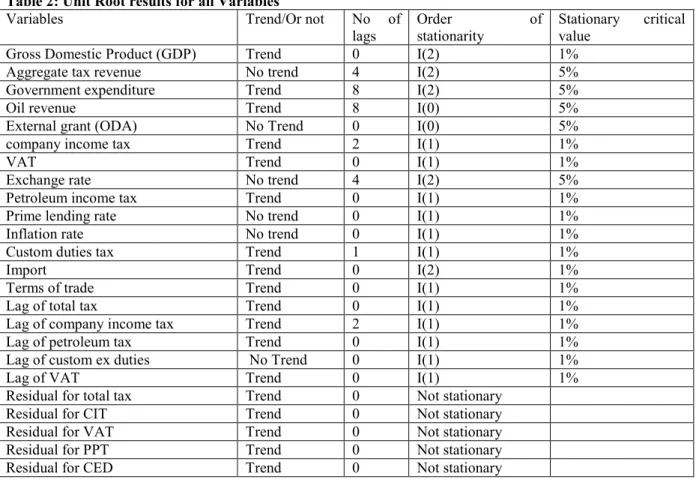
Table 2: Unit Root results for all Variables

Variables Trend/Or not No of

lags

Order of stationarity

Stationary critical value

Gross Domestic Product (GDP) Trend 0 I(2) 1%

Aggregate tax revenue No trend 4 I(2) 5%

Government expenditure Trend 8 I(2) 5%

Oil revenue Trend 8 I(0) 5%

External grant (ODA) No Trend 0 I(0) 5%

company income tax Trend 2 I(1) 1%

VAT Trend 0 I(1) 1%

Exchange rate No trend 4 I(2) 5%

Petroleum income tax Trend 0 I(1) 1%

Prime lending rate No trend 0 I(1) 1%

Inflation rate No trend 0 I(1) 1%

Custom duties tax Trend 1 I(1) 1%

Import Trend 0 I(2) 1%

Terms of trade Trend 0 I(1) 1%

Lag of total tax Trend 0 I(1) 1%

Lag of company income tax Trend 2 I(1) 1%

Lag of petroleum tax Trend 0 I(1) 1%

Lag of custom ex duties No Trend 0 I(1) 1%

Lag of VAT Trend 0 I(1) 1%

Residual for total tax Trend 0 Not stationary

Residual for CIT Trend 0 Not stationary

Residual for VAT Trend 0 Not stationary

Residual for PPT Trend 0 Not stationary

Residual for CED Trend 0 Not stationary

The above table shows us that most of the variables had unit roots and hence were not stationary, thereby requesting for differencing to make them stationary. However Oil revenue and external grant were stationary at level form. While the others were I(1) and I(2) process. The fact that there exists unit root for most of the variables is a necessary condition for co-integration. Co-integration is aimed at testing the long –run relationship of the variables, wherein if it is validated then it means there is a problem that needs to be corrected with the error correction model. Surprisingly in this study, the co-integration test which is the unit root test of the residuals of each regression suggests that there exist no co-integration in any of the regressions. This therefore implies that the sufficient condition for an error correction model is not satisfied; therefore we conclude that there exists no long-run relationship amongst the variables.

Regression results of Aggregate tax

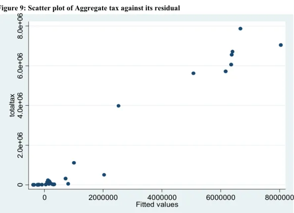
To achieve objective one, which is to investigate the elasticity and buoyancy of aggregate tax in Nigeria with respect to GDP, we ran the regression as specified in equation 1. However the study first of all tests for linearity of the dependent and explanatory variables as prescribed by the assumptions of the classical linear theory. To be able to do this, the researcher drew scatter plot of the dependent variable – aggregate tax against its residual and the outcome is shown on the figure below.

Figure 9: Scatter plot of Aggregate tax against its residual 0 2 .0 e + 0 6 4 .0 e + 0 6 6 .0 e + 0 6 8 .0 e + 0 6 to ta lt a x 0 2000000 4000000 6000000 8000000 Fitted values

The scatter plot above shows a 45 degree line pattern of the dependent variable and the residual hence suggesting that there exist a linear relationship between aggregate tax and its explanatory variables therefore validating the assumption of linearity for the regression whose results are stipulated below.

Table 3: Regression results for aggregate tax and its determinants

Variables Coefficients of determinants

lag1totaltax 0.295** (2.89) Realgdp 1.124 (0.38) Govexp 0.0745 (0.23) oilrevenue 0.447 * (2.23) extgrantna~a -53520.98 (-0.45) inflation -1858.5 (-0.30) Taxrefdummy 3219970.5*** (6.89) _cons -257965.9 (-0.40) N 31 R square 0.9868 Durbin Watson 2.683756 F- probability 0.0000 t statistics in parentheses * p<0.05, ** p<0.01, *** p<0.001

The regression result above suggests that the overall significance of the model is good as the F probability is very low (0.0000), and the R2 _{is equally very high (0.9868) suggesting that 98.68% of the}

dependent variable are explained by the explanatory variables. Also there exists no positive or negative strong auto-correlation in the regression since the Durbin Watson statistic (2.63) falls in the zone of indecision.

The main objective from this result is to ascertain the elasticity of aggregate tax with respect to the gross domestic product which is given by the coefficient of GDP (having linearized aggregate demand and GDP).

The degree of responsiveness of tax with respect to GDP is therefore given as 1.124. According to table 3, 1.124>1 implies that the responsiveness of tax with respect to a change in tax is relatively elastic. Though the elasticity is close to 1, the study opines that policies aimed at increasing the tax base can seriously consider increasing aggregate tax to some extend since it’s relatively elastic. This is important to Nigeria, given that over the years efforts have been made to improve on internally generated revenue. Aggregate tax can therefore accommodate an increase at least to some extent.

To ascertain the buoyancy of tax this study considered the 2004 tax reforms and stipulated a dummy to capture the structural break. The dummy variable is significant up to 99.9% confident interval thereby suggesting that aggregate tax was significantly buoyant to the tax reforms of 2004. This also implies that many more vision designed policies like such could be designed to improve the tax base of the economy. Apart from the main objective this result further show that the previous’ year’s tax is a positively significant determinant of current year’s aggregate tax. This is expected given that, Nigeria like many other African/developing countries produces their budgets based on last year’s income, and so targets are often set just a little above the previous year’s figure and not based on the country’s needs and wants.

Also, government expenditure and real GDP are not significant while oil revenue is a significant determinant of aggregate tax in Nigeria. However they are all positively and directly related to aggregate tax. This implies that government expenditure is not focused on taxable institutions and organizations which should ordinarily turnaround to generate revenue through tax. In addition gross domestic product also is not significantly based on tax in Nigeria due to the country’s overdependence on oil. While Oil revenue is shown to be a significant determinant of aggregate tax since most of the oil revenue mainly due to the large use of oil revenue in driving the economy. As Nigeria is still a major importer of refined crude and so oil revenue can better stimulate aggregate tax if well harnessed.

Furthermore, inflation and external grants are equally not significant but have a negative and inverse relationship with the aggregate tax of Nigeria. This implies that as tax inflation increases aggregate tax drops though this is not significant. This could be attributed to the fact that as inflation rises, some firms may close down hence reducing the amounts that would have been collected from them as tax. Also external grant or official development assistance tends to have an inverse relationship with aggregate tax and could be explained by the fact that most of these grants are usually not taxed, and some of these grants (such as health aids) reduces the private firms that would have sold the health facilities and hence the tax that would have been gotten. A good example is the huge sums of money that have been pumped into Africa and Nigeria in particular to eradicate malaria which is most times converted as mosquito nets and hence relegates traders that are involved in mosquito nets.

Regression results of the four major types of tax

The second objective of this study is aimed at investigating the elasticity and buoyancy of the four major taxes as designed by the scope. This section will use the same procedure as above, but only this time it will be the different main taxes. However we test for the linearity of all the four taxes as dependent variables and their residuals.

Figure 10: Scatter Plots of CED, PPT, CIT and VAT and their residuals

0 1 0 0 0 0 0 2 0 0 0 0 0 3 0 0 0 0 0 c u s to m a n d e x c is e d u ti e s 0 100000 200000 300000 Fitted values 0 1 0 0 0 0 02 0 0 0 0 03 0 0 0 0 04 0 0 0 0 0 c o m p a n y in c o m e ta x 0 100000 200000 300000 400000 Fitted values 0 2 0 0 0 0 040 0 0 0 060 0 0 0 080 0 0 001. 0 e + 0 6 p e tr o le u m p ro fi tt a x 0 500000 1000000 Fitted values 0 1 0 0 0 0 02 0 0 0 0 03 0 0 0 0 04 0 0 0 0 0 v a t -100000 0 100000 200000 300000 Fitted values

The figure above represents the scatter plots of the four major taxes under consideration which include; the custom and excise duties, company income tax, petroleum profit tax and value added tax against their various residuals. The four graphs depicts a 45 degree line pattern sloping from left to right which is what is normally expected of a linear trend. This therefore suggests that all the taxes tested above are linearly related to their explanatory variables and therefore validates the linearity assumption of the classical linear theory. Based on this result therefore the researcher can further regress the equations while testing for the other assumptions of the classical linear theory.

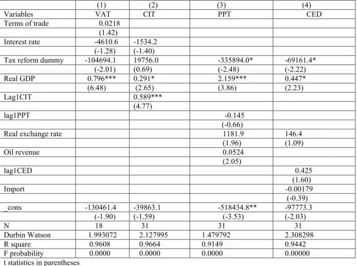
The table below therefore portrays the result of the regressions for all four taxes mentioned above. The table shows their coefficients, t-values, R squares and the F probabilities.

Table 4: Regression results for VAT, CIT, PPT and CED

(1) (2) (3) (4)

Variables VAT CIT PPT CED

Terms of trade 0.0218 (1.42)

Interest rate -4610.6 -1534.2 (-1.28) (-1.40)

Tax reform dummy -104694.1 19756.0 -335894.0* -69161.4*

(-2.01) (0.69) (-2.48) (-2.22) Real GDP 0.796*** 0.291* 2.159*** 0.447* (6.48) (2.65) (3.86) (2.23) Lag1CIT 0.589*** (4.77) lag1PPT -0.145 (-0.66)

Real exchange rate 1181.9 146.4

(1.96) (1.09) Oil revenue 0.0524 (2.05) lag1CED 0.425 (1.60) Import -0.00179 (-0.39) _cons -130461.4 -39863.1 -518434.8** -97773.3 (-1.90) (-1.59) (-3.53) (-2.03) N 18 31 31 31 Durbin Watson 1.993072 2.127995 1.479792 2.308298 R square 0.9608 0.9664 0.9149 0.9442 F probability 0.0000 0.0000 0.0000 0.00000 t statistics in parentheses * p<0.05, ** p<0.01, *** p<0.001

The result above suggests very significant models for all the taxes, given that the F probability remains 0.0000 for all four of them therefore implying that the overall model is highly significant. Also their R2 _{is very}

high as all of them are above 91% which implies that they are all highly explained by the determinants. The Durbin Watson statistic shows that there exist no autocorrelation for VAT and CIT while PPT and CED falls in the zone of indecision. This therefore implies that none of them are either positively or negatively auto correlated.

The major objective however is to ascertain the elasticity and the buoyancy of these taxes. Surprisingly unlike the aggregate tax, three of the taxes have their GDP coefficients lying between zero and one. This therefore suggests that VAT, CID and CED are all relatively inelastic and implies that they have a little proportionate change with respect to a unit change in GDP. Hence policies designed to increase or decrease these tax bases should be neglected, this is because the result proposes that a change in GDP will not over-change the tax volume of VAT, CID and CED. On the other hand petroleum profit tax (PPT) is relatively elastic, given that the coefficient of GDP is as high as 2.159 which is higher than the elasticity of the aggregate tax. This implies that PPT is highly flexible and hence responds with a more than proportionate change to a unit change in GDP. Nevertheless what is most interesting and of course expected is that, all taxes tend to increase with increase in GDP.

The test of buoyancy for all four taxes shows that VAT and CIT are not buoyant with respect to the 2004 tax reforms as their p-values are higher than 0.05 even though the dummy for VAT has a t-value of -2.01. While PPT and CED appear to be buoyant with their dummy values for structural break is significant at 95%

confidence interval. It is worth noting however that while CIT improved after 2004 (had a positive impact), the other taxes- VAT, PPT and CED did not.

Inferring from the determinants of VAT the result suggests that, terms of trade and interest rate are not significant determinants of VAT, while real GDP is significant at 99.9% confidence interval. As expected, interest rate has an inverse relationship with VAT. This could be explained by the fact that as interest rate (prime lending rate) falls more firms and industries will be motivated to produce (add value in all forms) and hence improving the VAT. On the other hand, terms of trade is positively related to VAT, implying that as terms of trade increases VAT equally increases. While the regression results of company and income tax (CIT) shows that, interest rate is still negatively related and not significant in determining CIT. However real GDP and the lag of CIT are significant in determining CIT. This therefore implies that the CIT of the previous year is significant in determining current CIT which is equally expected as most targets are usually made based on the previous year’s amount. Real GDP is equally significant and positive insinuating that an increase in GDP leads to an increase in CIT which is a good sign.

The regression results of petroleum profit tax (PPT) suggest that its lag, real exchange rate and oil revenue are all not significant determinants of PPT. However while real exchange rate and oil revenue are positively related, the lag of PPT is negatively related. The negative relationship of the lag may be explained by the volatility that exists in the oil market which might be later transferred to the tax collected from its proceeds. While real GDP and the tax reform dummy are significant determinants of petroleum profit tax.

The regression results of the custom and excise duties (CED) show that real exchange rate, imports and its lag are all not significant determinants, while real GDP and the dummy are both significant determinants at 95% confidence interval. However, real GDP, real exchange rate and the lag of CED are positively or directly related to CED, implying that as they increase, custom and excise duties increase as well. What is most surprising is that there exists an inverse relationship between imports as against custom and excise duties. This implies that as imports increase custom and excise duties drop which shouldn’t be the case. This could only be attributed to the huge corruption that exists in the importation of oil that constitutes a large amount of the country’s import.

Regression results of aggregate tax revenue during and after the oil-boom in Nigeria

To ascertain the significance of the structural break point this research first of all runs a Zivot Andrews unit root test on oil revenue to identify the structural break point and hence the oil boom dummy period.

Figure 11: Zivot Andrews Unit root test for oil revenue

-3 -2 -1 0 B re a k p o in t t-s ta ti s ti c s 1980 1990 2000 2010 year Min breakpoint at 2005

Zivot-Andrews test for oilrevenue, 1987-2006

The figure above represents the Zivot Andrews unit root graph results and indicates that the structural break point was 2005, it is also visible that the boom period experienced before 2005 and a depression on oil

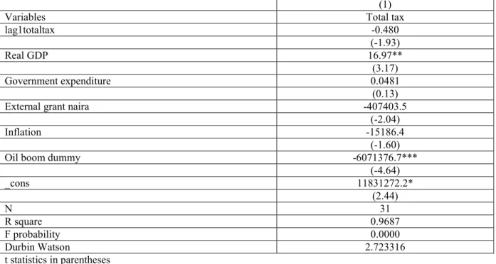
revenue was witnessed in 2005. The dummy period shall therefore be designed as 1 for 1980-2004 and 0 assigned to 2005-2011. The same regression for aggregate tax to ascertain if there was a significant structural break is therefore presented below.

Table 5: Regression results for Aggregate tax to determine the oil boom structural change

(1)

Variables Total tax

lag1totaltax -0.480 (-1.93) Real GDP 16.97** (3.17) Government expenditure 0.0481 (0.13)

External grant naira -407403.5

(-2.04)

Inflation -15186.4

(-1.60)

Oil boom dummy -6071376.7***

(-4.64) _cons 11831272.2* (2.44) N 31 R square 0.9687 F probability 0.0000 Durbin Watson 2.723316 t statistics in parentheses * p<0.05, ** p<0.01, *** p<0.001

The overall significance of the model is good as the F probability is as low as 0.000, with a high R2 _of

96.87%. Also there exist no positive or negative auto correlations in the model. The oil boom dummy shows that it’s significant at 99.9% confidence interval and has an inverse relationship with aggregate tax. This implies that after the boom period, aggregate tax fell significantly as compared to the boom period. This therefore conjectures that oil revenue was a significant contributor to aggregate tax especially in boom periods.

Summary

Many countries in the world have greatly sponsored their government expenditures with the aid of tax revenue, and owe their developments to this internally generated revenue. Nigeria started off on a good foot with the huge agro-production after her independence. However the discovery of crude attracted most investors to the oil sector thereby neglecting the other potential sectors that would have stirred up the industrial production and then increase tax revenue. The motivation of this study was therefore to find out how flexible tax is in terms of the elasticity and buoyancy, in an attempt to improve the tax base and generate more income. The study therefore investigates the elasticity and buoyancy of aggregate and four other major taxes with respect to economic growth in Nigeria. Also, the study analyzed the flow of oil revenue during and after the boom period.

To be able to capture these objectives the study uses the 2004 tax reforms to establish a dummy period and ascertain the buoyancy, while using the logged coefficient of GDP to aggregate tax and major taxes in order to determine the Growth elasticity of tax. For the third objective the study uses the Zivot Andrews structural break test to ascertain the most severe structural break of the oil revenue trend, and then uses simple OLS regressions with dummy effects to analyze the trend of aggregate tax with respect to the periods during and after the boom period.

The results of this research are far enriching as it suggest that aggregate revenue is relatively elastic. This implies that an increase in the GDP will increase tax to a more than proportionate level. Also the tax reform of 2004 was highly significant on aggregate tax and therefore infers that aggregate tax is relatively buoyant. The same test was done on four major taxes namely; value added tax, custom and excise duties, petroleum profit tax and company income tax. Out of the four taxes, only PPT was found to be relatively elastic while the other three were found to be relatively inelastic. However the results further suggest that, while VAT and CIT are not significantly buoyant according to the 2004 tax reforms, PPT and CED are significantly buoyant. The Zivot Andrews structural break unit root test was then used to ascertain the most severe structural break on the oil revenue trend and found it to be 2005. Then the study used the 2005 structural break to establish the dummy period during and after the oil boom. With the aid of the dummy the study regressed aggregate tax revenue against its determinants and the results showed that there was a significant drop in aggregate tax revenue after