Decentralisation, corruption and
economic development
Sebastian Freille
∗ University of NottinghamM Emranul Haque
University of ManchesterRichard Kneller
University of Nottingham March 2007 AbstractThis paper studies the relationship between corruption and decentralisa-tion from a macroeconomic perspective. Providing a macroeconomic analy-sis may help to understand better the links and channels between corruption, decentralisation and economic development. The analysis presented in this paper is unique in that provides an explicit formulation of the relationship between corruption, decentralisation and economic development. We bring together the theoretical and empirical predictions of both the traditional and modern fiscal federalism theories and find that the effect of decentral-isation on development depends crucially on the existence and extent of corruption. Without corruption, decentralisation is unambiguously the best outcome for development. However, if corruption is pervasive, decentrali-sation may be associated to lower capital accumulation than centralidecentrali-sation. This result is more likely to be observed in developing countries with weak local political institutions and significant information asymmetries between the government and local administrations.
∗Room C36, University Park, University of Nottingham, NG7 2RD, Nottingham, UK.
mailto:[email protected]
1
Background and motivation
Our motivation in this chapter stems from the need to address the relationship between decentralisation and corruption from a macroeconomic perspective, con-sidering the various interdependencies between these aspects. In order to do so, we bring together three different strands of literature to present an integrated analysis that has been relatively absent in the literature. Firstly, we invoke the traditional fiscal federalism literature and its effects on efficiency. The second strand is related to the role of information asymmetries and control mechanisms in hierarchical organisations. The final topic concerns the effects of bureaucratic corruption on economic development. The novelty of this study lies in the use of a dynamic growth model to analyse the relationship between decentralisation, corruption and growth. To the best of our knowledge this is the first study us-ing such an approach to analyse the relationship between these three variables1. Our main result highlights the role of corruption and information asymmetries in determining whether decentralisation is preferred to centralisation in terms of economic development.
The traditional theory of fiscal federalism provides strong implications in terms of the efficiency of the decentralised provision of public goods and services. The theoretical literature has recognised the positive effects that decentralised public spending has on growth. Since the early contributions of Samuelson and Mus-grave2, the theory of fiscal federalism has supported the view that decentralisation increases economic welfare by “tailoring outputs of such goods and services to the particular preferences and circumstances of their constituencies” [Oates (1999), p. 1122-23]. The Decentralization Theorem [Oates (1972)] establishes a presumption in support of decentralised provision of public goods and services on the grounds of efficiency. As Oates (1999) argues, this presumption is likely to be more justified in the presence of information asymmetries and political constraints. Additionally, the potential gains from decentralization increase if the demand for local public goods is highly inelastic, an idea that finds support in the econometric evidence. Furthermore, the welfare gains from decentralization are enhanced by the "voting 1Ellis and Dincer (2004) model the relationship between decentralization and corruption but
their study is based and formalized using the idea of yardstick competition.
2See Oates (2005) for a detailed review of these early contributions and their importance on
the fiscal federalism literature.
with the feet" and the mobile households arguments, although they are not depen-dent on that assumption. More recently, Brueckner (1999, 2006) has shown that federalism increases the incentive to save and ultimately leads to higher economic growth. The presumption of the existence of significant efficiency and welfare gains associated to the decentralised provision of public goods has also found support in recent empirical evidence [Yilmaz (1999), Lin and Liu (200), Akai and Sakata (2002), Thiessen (2003) and Stansel (2005)]3. In sum, there appears to be both theoretical and empirical arguments to expect a positive effect of decentralised provision of public goods and services on efficiency and welfare4
Other strand of the literature addresses the role of incentives, information asymme-tries and monitoring in organizations. More generally, this literature is concerned with the role of asymmetric information in a principal-subordinate relationship. One of the main implications of these models is that decentralisation in the context of hierarchical organisations may lead to higher corruption. In a very influential paper, Aghion and Tirole (1997) show that if the information asymmetry between principal and subordinate is significant,real authority rests with the subordinate. This also tends to raise the monitoring cost for the principal. As Carbonara (1998) notes in relation to Aghion and Tirole (1997), delegation of formal authority low-ers the principal’s incentive to perform their screening and detection activities, decentralisation encourage corrupt activities. The last paper shows that decen-tralisation of authority may increase corruption under some conditions. Similar ideas are also presented by Bac (1996) who argues that flatter hierarchies are pre-ferred when government monitoring is not specialized. In other words, due to the larger and wider span of control that the government has on steeper hierarchies, a more centralised organisation is more convenient. Both the bureaucracy and the government are hierarchical organizations and some of the aspects regarding its internal information and coordination relationships may be analysed and inter-preted using these theories. If we agree that decentralisation involve the creation of intermediate decisional layers consisting of public agents in charge of certain 3Earlier studies including Davoodi and Zou (1998) and Zhang and Zou (1998), Woller and
Phillips (1998) found no significant association between decentralisation and growth.
4There are three main drawbacks of federalism and decentralised provision of public goods:
the sacrifice of economies of scale in the provision of certain public goods and services, losses associated to inter-jurisdictional tax competition and the issue of public-good spillovers and inter-jurisdictional externalities. While these have been noted in the literature, their extent and significance appear to limited to specific sets of public goods and services, taxes and infrastruc-ture expendiinfrastruc-tures.
decisions, then these ideas of formal and real authority, information asymmetries and deficient monitoring are certainly important in the debate of the relationship between decentralisation and corruption.
Finally, the third strand of the literature we bring into our theoretical model is related to the effect of corruption on economic development. Although some time ago there were suggestions that bureaucratic corruption could foster efficiency and development, the view in recent decades is that corruption has a negative effect on economic development. This effect operates through different channels among which the diversion of resources away from productive activities is one of the most important. This has been suggested both in theoretical studies [Murphy et al. (1991, 1993), Romer (1994)] and empirical studies [Mauro (1995), Brunetti (1997), Hines (1995) and Kaufmann et al. (1999)]. At the same time, there is a growing literature that acknowledges the existence bi-directional relationship be-tween corruption and development. The main proposition of these studies is that bureaucratic corruption and development are jointly determined where equilib-rium behaviour is dependent on the decisions of other agents. Multiple equilibria are typical in these models which predict a two-way negative relationship between corruption and development. This literature also explains the existence and persis-tence of corruption as a permanent feature of the economy [Ehrlich and Lui (1999), Mauro (2004), Aidt et al. (2005) and Blackburn et al. (2006)]. These theoretical presumptions have received some support in a few empirical studies [Haque and Kneller (2004), Aidt et al. (2005) and Mendez and Sepulveda (2006)] who have found a non-monotonic relationship between corruption and development.
Having already established the motivation of our research, it is important to note the relevance of the topic analysed in this chapter. The relationship between de-centralisation and development has received an increasing share of research effort over recent decades. This is in part a consequence of a global trend towards devo-lution and decentralisation5, most notably in developing and transition economies. 5 Although often used as equivalent, concepts such as decentralisation, deconcentration and
devolution refer to slightly different and particular aspects of the relations between central and periphery governments. We will refer to decentralisation to describe any type of power shift away from the centre while we will use different concepts of decentralisation (administrative, fiscal, political, etc.) in different sections of this chapter. Manor (1999) describes the different concepts of decentralisation in the following three types: a) deconcentration or administrative decentral-isation; b) fiscal decentraldecentral-isation; and c) devolution or democratic (political) decentralisation. Other useful references on this are UNDP (1999) and Treisman (2002).
A large number of countries have implemented programmes and strategies to redesign the relationship between different levels of government [Manor (1999), UNFPA (2000), Rodriguez-Pose and Gill (2003)]. Industrialized countries have voluntarily taken steps to decentralize the provision of certain public services and adopted more decentralised schemes of power sharing. In these countries, the main objective has been to improve the delivery of public services and to adapt govern-ment structures to better suit the needs of the citizens. This is for example, the case of the decentralisation of service delivery in the UK since the early 1980’s. The introduction of neighborhood offices to improve access to certain services had limited success but created the foundations for other reforms as in the case of the decentralisation of the UK health system [Leach et al. (1994)]. Similarly there have been significant transfers of powers to the National Parliaments of Scotland, Wales and Northern Ireland.
In the case of developing countries, the decision to redefine the relations between government levels was mainly driven by the recommendations from international organizations such as the World Bank and the United Nations. The main objec-tives behind such recommendations were those of promoting development through the rearrangement of fiscal, political and administrative relations between govern-ments and strengthening civil and democratic institutions. Whether voluntarily adopted or externally dictated, there is little doubt that decentralisation strategies have been encouraged primarily on the grounds of the perceived benefits found in the traditional theory of fiscal federalism, i.e. efficiency in public provision and intergovernmental competition and greater matching of local needs with provi-sion. In addition to this, decentralisation has also been supported by the view that centralised socialist regimes failed to generate conditions leading to sustained growth. The experiences of China, India and Russia are good examples of this. In any case, as Manor (1999) argues, almost every country has adopted some form of decentralisation over the last decades based on the general presumption that it would provide a solution to many different kind of problems which centralised regimes had failed to address.
It does not follow however, even if centralised regimes have little credit on em-pirical (or anecdotal) grounds, that the more decentralised structures are bereft of such problems. While the transition to decentralisation may address several of the efficiency issues mentioned before, it creates new problems. For example,
local capture of governments and inappropriate accountability systems may stand in the way of the decentralisation process and overturn the benefits of allocative efficiency. Other sources of complications include the existence of agency prob-lems, information asymmetries, deficient monitoring of sub-national governments and problems arising due to vertical fiscal imbalances. These and other related topics form an important part of the recent and current research on fiscal federal-ism and decentralisation which aims to integrate political economy considerations in the traditional approach. As noted by Bardhan (2002), these considerations are specially relevant in developing countries where the political and institutional framework at the sub-national level is often very weak. Learning why and how these problems arise and develop under different governmental arrangements and the consequences they have for development is essential in order to inform the discussion on these matters. Our aim in this chapter is to contribute to the under-standing of the complex interactions between decentralisation and development by focusing on a specific aspect of this relation, namely corruption.
Public sector corruption affects development in several ways, the more obvious being the allocation of resources away from productive activities and the squan-dering of public funds. There are however more subtle ways in which corruption may distort incentives and modify behaviour of economic agents bearing impli-cations for development. Once recognised, it becomes clear that the analysis of the relationship between corruption and development should be approached using many different configurations of assumptions. These efforts have produced a large body of literature studying this relation at several levels6.
Among the most debated topics in the decentralisation and development litera-ture, an interesting idea concerns the possibility that the nalitera-ture, extent and effects of bureaucratic corruption may be sensitive to the design of the relations between (and within) different levels of government. This suggestion, made by Shleifer and Vishny (1993), Prud’homme (1994), Oates (1999), and Bardhan (2002), has intro-duced yet another level to the debate on the benefits of decentralisation for both industrialized and developing countries. If we consider this possibility seriously, then it is important to incorporate these considerations into any analysis of the 6For an excellent survey on corruption and development see Bardhan (1997). Aidt (2003)
surveys a number of theoretical approaches to corruption and Jain (2001) reviews some important theoretical and empirical aspects of corruption.
problems of corruption and test the robustness of results.
The potential importance of institutional features in a world of increased decen-tralisation noted above forms one of the main motives for this study. There are several reasons to believe that the nature and scope of bureaucratic corruption are likely to be different under centralised and decentralised government structures. Some of these reasons have been analysed in the literature of the new political economy of decentralisation in the form of information asymmetries [Bird (1994)], political accountability [Seabright (1996)], capture by elite groups [Bardhan and Mookherjee (2000)], yardstick competition [Besley and Case (1995)], conflict of interests [Blanchard and Shleifer (2001)], and structural organisation of bribery [Shleifer and Vishny (1993)]. Some of these elements may influence the decision of a bureaucrat to be corrupt and they may also affect the extent of corruption in an economy. Hence, we will study the suggestion that the effect of centralisation and decentralisation on development may depend on the nature and extent of corrup-tion using a dynamic general equilibrium approach. We develop this framework in the next section and specify the potential implications that this may have on policy design and implementation.
Reviewing the anecdotal and case-study evidence over the last two or three decades, we find a common pattern of meagre success (if any) of decentralisation pro-grammes among developing countries. This is the case for example of Indonesia, a highly centralised country which has implemented a decentralisation process with very unimpressive results to date7. Some Latin American countries, like Argentina, Chile and Colombia, experienced mixed results following the decentralisation of certain public services and in particular of education during the 80’s and early 90’s. On one hand, some improvements were achieved in terms of educational indicators but on the other hand, the sub-national levels found extremely burden-some to cope with the new services and this led to overspending, mismanagement, and rising provincial and municipal debts. In all cases, the way in which the ac-countability relationships were set to work determined the success or failure of the decentralisation programme. With the exception of Nicaragua and El Salvador, all the countries failed to ensure these accountability relationships and decentrali-7Some of the obstacles the decentralisation program has encountered in Indonesia are
de-scribed inDecentralize Indonesia without dismantling it, International Herald Tribune, 23 Jan-uary 2001.
sation brought along new problems8. These examples also extend to some African countries where problems of accountability and corruption have sprung following decentralisation attempts.
This chapter study the relationship between corruption and decentralisation from a macroeconomic perspective. Given that the effects of any decentralisation pro-gramme are ultimately spread to the aggregate variables, this has some value. Providing a macroeconomic analysis may also help to understand better the links and channels between corruption and economic development. We put the em-phasis on the relation between the existence of corruption, the power-sharing ar-rangements between the governments and economic development. The analysis presented in this model is unique in that provides an explicit formulation of the relationship between corruption, decentralisation and economic development. We bring together the theoretical and empirical predictions of both the traditional and modern fiscal federalism theories and find that the effect of decentralisation on de-velopment depends crucially on the existence and extent of corruption. Without corruption, decentralisation is unambiguously the best outcome for development. However, if corruption is pervasive, decentralisation may be associated to lower capital accumulation than centralisation. This result is more likely to be observed in developing countries with weak local political institutions and significant infor-mation asymmetries between the government and local administrations.
The remainder of this chapter is organised as follows. The next section presents the model introducing the agents and their motivations. Section 3 analyzes the in-centive condition for agents to be corrupt and examines the presence of corruption in the model. In section 4 we derive the expressions for the budget equation and taxes under corruption and no-corruption. Section 5.1 deals with the case of a cen-tralised economy under corruption and no-corruption. Section 5.2 analyzes what happens when the economy is decentralised and the corresponding implications for corruption and development. Section 6 concludes.
8Di Gropello (2004) provides a detailed account of several experiences of educational
decen-tralisation in Latin American countries and their rather unimpressive results. The substantial overspending and lack of accountability of sub-national administrations following these and other decentralisation programmes has been a cause of concern ever since.
2
The Model
We develop a dynamic macroeconomic growth model with public services [Barro (1990)], corruption, poverty traps and development [Ehrlich and Lui (1999), Mauro (2004), Blackburn et al. (2006)]. These models have certain common features, most important amongst which include the existence of multiple equilibria and de-velopment traps originating from the interaction between opposing forces. While Ehrlich and Lui (1999) put the emphasis on the trade-off between socially unpro-ductive political capital and growth-enhancing human capital, Mauro (2004) and Blackburn et al. (2006) base their analysis around the incentives faced by officials to engage in corruption. Our model follow more closely the latter.
2.1
Environment
Time is discrete and indexed byt= 0,1, ...,∞. All agents live for two-periods only and belong to overlapping generations of dynastic families. There are two groups of agents -households and bureaucrats9. Total population is constant and normalised to 1, a proportion m of which are households and n are bureaucrats (n < m). All agents work and save during the first period and consume only in the second period. Households work for private firms in exchange for a wage while bureaucrats work for the government implementing policy. Policies are designed by politicians, who are part of the government, and it is they that are in charge of monitoring the activities of the bureaucrats10. Public policy consists of a package of taxes and expenditures,G, destined to provide public goods and services. Corruption arises when, under certain conditions, bureaucrats are willing and able to appropriate public funds in an unlawful manner thereby reducing the effective level of provision of public goods and services destined to productive activities. In order to avoid certain rigidities imposed by the settings of our model, we assume that, no matter how strong the incentives to engage in corruption, there will always be a core of 9We assume away the occupational choice problem by making agents differentiated at birth.
The skills required to become a bureaucrat are only possessed by a fraction of the population. Later on, when we refer to the behaviour of bureaucrats, we specify a condition by which they are induced to take public office rather than working in the private sector.
10For simplicity, we see the government as a benevolent policy maker. As we are only dealing
with bureaucratic corruption, we do not consider the possibility of elections incentives or a corrupt government in our chapter.
non-corruptible (and hence non-corrupt) agents. In this way, we assume that a proportion ν ∈ (0,1) of all the bureaucrats are corruptible while the remaining
1−ν are non-corruptible, and by definition, never corrupt11. On the other hand, all the other agents undertake activities in the private sector and their behaviour may be indirectly influenced by bureaucratic behaviour. Households work for private firms who, in turn, combine labour and capital to produce final output. All markets are perfectly competitive and payments to the productive factors are equal to their marginal products.
2.2
Households
Young households -households in the first period- are endowed withλ >1units of labour which they supply inelastically to firms in return for a wagewt. Total labour supply in the economy amounts to lt =λm. In addition to their labour income, each young household receives a bequest bt from the previous generation12. They are also liable to pay taxes out of their gross income. For simplicity we assume they pay a lump-sum tax τt and their net lifetime income is therefore equal to
λwt−τt+bt. Households save their entire net income at the market interest rate to pay for private consumption and bequests left at the end of their lives in the second period13. Each household derives linear utility from their consumption of private goods and also from their donations to their offspring. Consequently, his lifetime income and utility are given by:
yih = (1 +rt+1) [λwt−τt+bt] (2.1)
Uih = (1 +rt+1) [λwt−τt+bt]−bt+1+u(bt+1) (2.2)
11We should also note at this point that the identity of a bureaucrat, that is whether he is of
the corruptible or non-corruptible type, is unobservable to the government.
12The introduction of bequests into the model is made for purely technical reasons. As we
are not interested in modelling bequests motives, we therefore choose a very simple formulation and with warm-glow altruism where parents leave a part of their earnings to their offspring and derive utility from this donation as originally suggested by Yaari (1965).
13In our model, unlike similar papers in the literature, households savings are not directly
affected by the activities of bureaucrats but rather indirectly via the effect embezzlement of government funds has on the level of taxation.
where rt+1 is the market interest rate on household savings and u(bt+1) is a
non-decreasing and strictly concave function that reflects the “joy-of-giving” motive associated to leaving bequests. Utility is maximized by the household by setting
ub(·) = 1 which implies a fixed-amount intergenerational bequest equal to b for all t. We should note that households earnings (and savings) are only affected by changes in wages and the tax level. As we shall see in the next sections, bureaucratic behaviour will affect these and may have important implications for the level of development.
2.3
The Government
The government enters the model through the effect public spending has on pri-vate output. In particular, we assume as in Barro (1990) that spending in public goods and services,G, is an input to the production function. Each unit of public spending G yields an amount σG, (σ ≤ 1) units of productive service. Once the government decides on the total amount of public spending, it then delegates the implementation and arrangements to bureaucrats. It is important to note that in our model the design of policies is the sole responsibility of the government (politicians)14. Bureaucrats only have authority over the implementation of public policies15. Designing a policy package entails deciding the amount of public spending to be allocated to each bureaucrat gi
t such that n P
i=1
gi = ng =G. Politi-cians will then allocate the funds to the respective bureaucrats who will carry out the implementation of the policies. We also note that bureaucrats are respon-sible for the collection of taxes from households but we rule out the possibility of collusion between bureaucrats and households to avoid the payment16. As in previous analysis [Blackburn et al. (2006), Blackburn and Forgues-Puccio (2006)] we assume that the government pays each a bureaucrat a wage equal to the one paid by firms in the private sector. In doing so, the government ensures complete 14Alesina and Tabellini (2004) consider a model where politicians and bureaucrats have
dif-ferent objectives and where elections have a role in the model. The objective of that paper is different to our objective here although it would be possible, in principle, to incorporate elections and politician incentives in our model.
15Although this may be seem as too extreme, it is in fact true that in most policy areas
bureaucrats act under the supervision of politicians and have only marginal or limited authority over many decisions. See Peters (2001) for reference.
16This activity may generate opportunities for public abuse in the form of bribery and tax
evasion. However, as all households have the same labour endowment and income, and are also subject to the same tax liability, corruption of this form does not arise in our model.
bureaucratic participation. If a bureaucrat is discovered to be corrupt, the gov-ernment fires him and strips him off his wage while recouping a fraction δ of the amount stolen.
The government finances its public expenditures by running a continuously bal-anced budget. Government revenues consist of taxes imposed on households plus any fines collected from bureaucrats who are found corrupt. The government knows the amount of tax revenue it should collect in the absence of corruption since it sets the tax rate and knows the number of tax-paying households17. If rev-enues fall short of this amount then the government will suspect that corruption is taking place. In this case, the government decides to investigate the activities of bureaucrats by using an imprecise costless monitoring technology18. In any case, the government is only able to detect and punish corrupt bureaucrats with a probability p∈(0,1) and with probability 1−pthe governments fails to capture the wrongdoers.
2.4
Bureaucrats
Following Ehrlich and Lui (1999) we assume that government intervention in the economy necessitates the existence and active participation of a bureaucratic sec-tor19. As we have already mentioned, bureaucrats are appointed by the govern-ment (politicians) to implegovern-ment a set of public policies. We assume that the bureaucratic sector has an informational advantage over the government and this asymmetry is also behind the inability to precisely monitor corrupt officials20. Al-17We abstract from considering other problems that may affect the certainty of tax revenues
such as tax evasion.
18For the sake of simplicity and to save on notation, we assume that government monitoring
is costless. This may be reasonable if we think that ex-post monitoring is a rather negligible fraction of total government expenditures. In any case, costly monitoring could be added into the model in a straightforward way without modifying the main results. In fact, it would strengthen our results since costly monitoring of corrupt bureaucrats adds an extra loss of resources to the economy.
19The complexity of modern government structures makes it impossible for the government to
make policy interventions without recurring to bureaucrats. As noted by Banerjee (1997) and Acemoglu and Verdier (1998), the agency problems created as a consequence of this are one of the crucial issues behind the existence of bureaucratic corruption.
20There are a number of treatments that examine in detail the role of public bureaus. In
par-ticular, Peters (2001) provides such an account and a detailed account of the nature, behaviour and motivations of modern bureaucracies. We assume that bureaucrats have no power over the design of policies, they are only able to alter its implementation.
though not directly accountable to the citizens they are certain to be fired by the government if found corrupt while holding office.
All bureaucrats earn a wage wBt for supplying inelastically their unit of labour endowment. Like households, bureaucrats save their total income during the first period for consumption in the second period. For simplicity, we assume that wages are the only source of legal income for bureaucrats and that these are equal to the wages paid in the private sector by firms. We have already noted that there are two types of bureaucrats -corruptible and non-corruptible-. By definition, a
non-corruptible bureaucrat is never corrupt and resorts to his legal income only. Accordingly, his income is always certain and equal to wb
t = wt. The lifetime income and utility of a non-corruptible bureaucrat are therefore given by:
ync,b =wtb (2.3)
Unc,b =wbt(1 +rt+1) (2.4)
A corruptible bureaucrat may or may not decide to engage in corruption. In particular, any such bureaucrat will evaluate the (expected) benefits of engaging in corruption against the benefits of remaining honest. If he decides against engaging in corruption, then his income and utility are given by equation 2.3 and 2.4. If a bureaucrat decides to engage in corruption he embezzles a fraction θti ∈ (0,1) of his public funds allocationg. For simplicity we assume that each bureaucrat steals the same fraction out of government funds, henceθt=θ21. Therefore, the income of a corrupt bureaucrat is equal to wb
t(1 +rt+1) +θtg with probability(1−p) and with probability p he is caught and fired earning (1−δ)θtg22. We can write the 21Naturally, the fraction a given bureaucrat may be able to steal depends on several factors.
One of them is the probability of detection which in our model is constant for a same-level bureaucrats as we later explain. Another factor is the “office power” of a bureaucrat relative to other bureaucrats. Although it is likely that there are differences in this, we assume the simplest case where all bureaucrats are alike in terms of “office power”. We discuss this issue in more detail later in the chapter.
22To leave things simple, we rule out the possibility of investing embezzled funds in either the
formal or informal sector. In this way, bureaucrats have to spend or hide their illegal income. Other possibilities have been analysed in the literature, such as spending additional resources to avoid being caught [Blackburn et al. (2006)] or by shipping the embezzled funds abroad [Blackburn and Forgues-Puccio (2006)].
expected income and utility of a corrupt bureaucrat as:
Ub,c =wtb(1 +rt+1)(1−p) +θtg(1−pδ) (2.5)
2.5
Firms
Output is produced by firms which hire labour from households and rent capital (loans) from all agents. There is a unit mass of identical output producers. The representative firm maximizes profits. The production technology of the represen-tative firm is given by:
yt =AlαtK α tk 1−α t G β A >0 ; α, β ∈(0,1) (2.6) where lt are labour units, Kt denotes the aggregate stock of capital and Gt de-notes total amount of productive services yielded by public spending23. Labour is hired at the competitive wage rate wt and capital is rented at the compet-itive rate rt. Profit maximization implies wt = αAlαt−1Ktαk
1−α t G β t and rt = (1−α)Alα tKtαk −α t G β
t. Since in equilibrium lt = l = λm and kt = Kt, we can write these as:
wt = αA(λm)α−1Gβkt≡w(kt) (2.7)
rt = (1−α)A(λm)αGβ ≡r (2.8)
We can observe that the wage rate is proportional to the capital stock whereas the equilibrium interest rate is constant.
23We incorporate both an economy-wide capital as in Romer (1986) and the services provided
by the public goods and services into the production function as in Barro (1990) as inputs enhancing the efficiency of private production.
3
The incentive to be corrupt
Having presented the utilities and optimization conditions for all the agents, it should be clear by now that corruptible bureaucrats face a decision on whether to engage in corruption or not. In particular, they will do so if their expected benefits are no less than the benefits of remaining honest. From equation 2.5 and noting that rt=rt+1 =r we can write this condition as:
wt(1 +r)(1−p) +θg(1−pδ)≥wt(1 +r) (3.1) where the left-hand side term is his expected utility of embezzling funds and the right-hand side term is his utility if he is honest. This expression can be rearranged conveniently to yield:
θg(1−pδ)≥pwt(1 +r) (3.2)
One crucial aspect of condition 3.2 is that it includes the economy-wide variables
wt and r. As we will see, both variables are functions of the aggregate level of corruption in the economy. This means that the motivation for a bureaucrat to engage in corruption will be affected by the decisions adopted by fellow bureau-crats.
We can start exploring these motivations by analyzing two alternative and extreme scenarios, one in which all bureaucrats are honest and one in which all bureaucrats are corrupt. We should remember at this point that corrupt behaviour affects the economy through a reduction in the available amount of public productive services which are themselves an input into the production function of output by firms. In this sense, only the “final” amount of public goods and services enters the production function and is denoted by Gt in equations 2.7 and 2.8. This means that, if corruption exists, there will be a difference between the amount of public funds the government decided to provide and the amount of public funds destined to productive activities.
We start by considering the case where all corruptible bureaucrats are honest. In this case, total government expenditure equals total public services delivered
yieldingG= ˆG=nσgin productive services. Accordingly, the incentive condition 3.2 becomes: θg(1−pδ)≥(1 + ˆr)pwˆt≡ζˆ(kt) (3.3) where ˆ r = (1−α)A(λm)ασβ(ng)β (3.4) ˆ wt = αA(λm)α−1σβ(ng)βkt ≡wˆ(kt) (3.5) The incentive condition given in 3.3 is the incentive condition for an individual bureaucrat to be corrupt given that no other bureaucrat is corrupt.
On the other hand, if all corruptible bureaucrats decide to engage in corruption and they embezzle a fractionθ out of public funds, then the total amount of public productive services delivered will be equal to G= ˜G=nσg(1−θ). The incentive condition in this case becomes:
θg(1−pδ)≥(1 + ˜r)pw˜t≡ζ˜(kt) (3.6) where ˜ r = (1−α)A(λm)ασβ(ng)β(1−θ)β (3.7) ˜ wt = αA(λm)α−1σβ(ng)β(1−θ)βkt≡w˜(kt) (3.8) Expression 3.6 is the condition for and individual corruptible bureaucrat to engage in corruption given that all other corruptible bureaucrats are also corrupt.
We can see that the only difference between the two set of equations for the wage rate and interest rate is the presence of the term (1−θ) as an argument of these
expressions for the all-corruption case. Given that(1−θ)is between 0 and 1 (since
0 < θ < 1), it is clear that for any given stock of capital the wage rate is lower under corruption than under no-corruption. Similarly, if we compare equations 3.4 and 3.7, we see that for any given stock of capital the interest rate is also lower when corruption exists. The economic explanation of this is that the total amount of public productive services under the presence of corruption is smaller
( ˜G <Gˆ), which reduces the productivity of the other inputs in the production of private goods.
4
Corruption and public finances
In the previous section, we established the condition for a bureaucrat to be corrupt under two different hypothetical scenarios. We also showed how the existence of corruption affected certain economy-wide variables such as wages and interest rates. We also noted earlier that changes in households (and bureaucrats) savings were triggered by changes in taxes and wages. It should be clear that wages are affected in the presence of corruption and that this affects the net earnings (and savings) of both households and bureaucrats. Now we study how are taxes affected by the existence of corruption and the effect this has on savings.
Since the government maintains a balanced budget each period it is essential to examine the budget equation under the two proposed scenarios for the level of taxes will be different in each case. First, if corruption is absent in the economy, government expenditures comprise wages paid to bureaucrats and spending on publics goods and services. Revenues consist of tax receipts from all households. In this case, the budget equation looks like:
mτ =ng+nwˆt (4.1)
We can determine the amount of taxes levied on households when all corruptible bureaucrats are honest as the following:
τ = ng+nwˆt
In comparison we consider the situation where all corruptible bureaucrats are indeed corrupt. In this case, each bureaucrat embezzlesθg with probability(1−p)
and if caught and fired (with probability p), he retains θg(1−δ). Accordingly, government expenditures comprise wages paid to bureaucrats and spending on public goods and services. However, unlike the previous case, both total wages and spending are affected. This occurs in part because there is a proportion of corrupt bureaucrats who are caught and dismissed without pay, government expenditure on wages are reduced by npνw˜t -the salaries of corrupt bureaucrats who are fired. It also occurs because as bureaucrats steal government funds that otherwise would have constituted tax receipts, the government lossesnνθg(1−pδ)
in public funds to corrupt bureaucrats that get away with their malfeasance24. Under these conditions, the budget equation becomes:
mτ =ng+nw˜t(1−pν) +c+nνθg(1−pδ) (4.3) and the level of taxes levied on households when all corruptible bureaucrats are corrupt is given by:
τ = ng+nw˜t(1−pν) +c+nνθg(1−pδ)
m ≡τ˜ (4.4)
Comparing equations 4.2 and 4.4, we see that the level of taxes under corruption may be higher or lower than under no-corruption. This is because while corruption results in the loss of public funds (embezzled funds), it also leads to lower payments of wages to bureaucrats (given that a fractionpof bureaucrats are caught and fired without pay). In fact, taxes under corruption will be higher only ifnw˜t(1−pν) +
nνθg(1−pδ)> nwˆt. Note that we can see the total amount of embezzled funds
nνθg(1−pδ)as an indication of the aggregate impact of corruption. Accordingly, the incidence of corruption in the economy will be larger the higher the fraction of corruptible bureaucrats,ν, the higher the funds allocated to each bureaucratg, the lower the probability of detectionp, and the lower the fraction the government is able to recover out of funds embezzled by bureaucrats who are caughtδ. We are now ready to analyse how corruption affects capital accumulation in the economy. 24Note that this amount is the result of the total amount of embezzled fundsnvθg minus the
We explore this possibility by analysing two alternative scenarios.
5
Regimes and development
In this section we address the issue of determining different regimes of corruption and development by focusing on the structural organisation of public service de-livery. In particular, we focus on two alternative extreme cases, full centralisation and full decentralisation. In order to incorporate the fiscal federalism propositions into this model we assume that regardless of whether corruption exists or not, de-centralised provision of public goods and services is more (economically) efficient than centralised provision. This assumption is meant to capture the differences -widely acknowledged and recognised in the literature- in the efficiency of public service delivery between centralisation and decentralisation. To keep the analysis simple, we assume that the parameterσ, which represents the economic efficiency associated to the provision of public goods and services, is larger under decen-tralisation than under cendecen-tralisation. In particular, we assume that σc < 1 and
σd= 1. We analyse the case of centralisation first.
5.1
Centralisation and development
In this section, we consider the case of an economy where the provision of public services is carried out by central level bureaucrats only. Probably the best way to think about this situation is one where local or regional bureaucrats have limited powers or no powers at all. In such a case, top-level or central bureaucrats are re-sponsible for the nationwide administration and delivery of public services. In such a configuration, we assume that the informational asymmetry problem between central bureaucrats and the government is limited. Even when the bureaucrats at this level may be better informed than the government about embezzlement op-portunities, the fact that these bureaucrats are “closer” to the central government (not only in geographical terms but more importantly in hierarchical terms) eases the monitoring tasks by the government. It is well agreed that monitoring and auditing are better developed and more efficient at the national than at the local or regional level [Prud’homme (1995)]. Additionally, one may think that in this type of setting bureaucrats constitute a more or less homogenous and cohesive
group which facilitates the monitoring tasks. The introduction of this assumption will affectθ which is labeled θc in this scenario.
We can now study how accumulation takes place in a corruption-free environment. In this case, both households and bureaucrats save their legal income. The sum of net savings by households and bureaucrats yields the total amount of savings in the economy as follows:
ˆ
st=m(λwˆt−τˆt+b) +nwˆt (5.1) where m(λwˆt−τt+b) are total household savings and nwˆt are total bureaucrat savings. Using equations 3.5 and 4.1 to rewrite equation 5.1 it follows that capital accumulation occurs in the following way:
ˆ
ktc+1 =αA(λm)α(σc)β(ng)βkt−ng+mb≡fˆc(kt) (5.2) Now we consider the case where the economy is affected by corruption. As we know from the previous discussion, this is the case where all corruptible bureaucrats are corrupt. In this situation, total savings comprise the net total savings by households plus the savings of all bureaucrats which are different from the non-corruption case. Note also that a number(1−ν)nof bureaucrats (non-corruptible) are able to save their legal income, but the group of corruptible bureaucrats will have an expected level of savings equal to νn(1− p) ˜wt. Thus, the wage that both corruptible and non-corruptible bureaucrats receive is lower than wage in the non-corruption case. In this way, total savings are given by:
ˆ
st=m(λw˜t−τ˜t+b) + (1−ν)nw˜t+νn(1−p) ˜wt (5.3) Replacing w˜t and τ˜t by their equals in equations 3.8 and 4.4 and plugging them into 5.3, we can derive the capital accumulation equation for the case where all corruptible bureaucrats are corrupt as:
Working with 5.2 and 5.4, we can find the steady state levels of capital for each case as the following:
ˆ kc,∗ = mb−ng 1−αA(λm)α(σc)β(ng)β (5.5) ˜ kc,∗ = mb−ng[1 +νθ c(1−pδ)] 1−αA(λm)α(σc)β(ng)β(1−θc)β (5.6) These steady state levels of capital are stationary if both mb > ng[1 +νθ(1−pδ)]
and if αA(λm)α(σc)β(ng)β ∈(0,1)are satisfied25.
From equations 5.5 and 5.6, it is evident that capital accumulation is lower under corruption than under no-corruption, that is k˜c,∗ < kˆc,∗26. The intuition behind this can be seen by remembering how corruption affects the main variables. First, as we have already noted, at every level of capital, the marginal productivity of labour is lower under corruption than no-corruption. The rationale behind this is that when bureaucrats embezzle public funds, the amount of public spending injected in the economy is lower and this reduces the productivity of labour and hence wages. Second, corruption raises the total costs of public goods causing taxes to be higher and resulting in lower total savings.
It is important to stress the result that corruption is harmful to development and that this is due to the loss of public resources and the decrease in public spending in goods and services. Furthermore, we are able to establish that corruption not only affects development but low development affects corruption. This follows from section 3 noting that ζˆ(kt) > ζ˜(kt). One can clearly observe that both conditions are increasing monotonically in kt. It is easy to show that there exist two critical levels of capital k1∗ and k2∗ such that:
Definition k1,b is the unique value of kt for which ζˆ(k1,b) =θg(1−pδ)such that
ˆ
ζ(·)< θg(1−pδ)for all kt< k1,b and ζˆ(·)> θg(1−pδ)for all kt> k1,b.
25Note that if mb > ng[1 +νθ(1−pδ)] then it is true that mb > ng. The same observation
is valid for the other condition since if αA(λm)α(σc)β(ng)β ∈ (0,1) then it is also true that αA(λm)α(σc)β(ng)β(1−θc)β∈(0,1).
26This follows from the evidence that for any givenk
Definition k2,b is the unique value of kt for which ζ˜(k2,b) =θg(1−pδ)such that
˜
ζ(·)< θg(1−pδ)for all kt< k2,b and ζ˜(·)> θg(1−pδ)for all kt> k2,b.
It is clear that k1,b < k2,b and that these capital levels define boundaries beyond which the incentive conditions given in section 3 are satisfied or not. Using these critical capital levels, we can now determine whether corruption forms part or not of an equilibrium. In particular, if kt < k1,b, there exists an equilibrium in
which all corruptible bureaucrats are corrupt. And if kt > k2,b, there exists an equilibrium in which all corruptible bureaucrats are non-corrupt. Finally, ifk1,b<
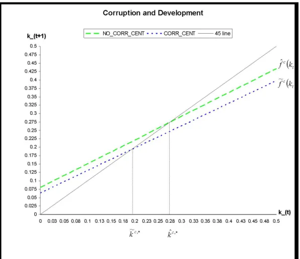
kt < k2,b, it results in multiple equilibria where bureaucrats are either corrupt or non-corrupt. These two results validate the other side of our argument, i.e. that low levels of development are associated to high corruption and viceversa27. As we can infer, these results give rise to three different development regimes. The first, a low-development regime where there is a unique stable equilibrium and for which corruption is part of the economy (in fact, corruption is at a maximum in this regime). The second, a high-development regime where there is a unique stable equilibrium and for which corruption is not part of the economy (there is zero corruption). Finally, an intermediate-development regime where there are multiple equilibria which are frequency dependent, i.e. the decision of a corruptible bureaucrat to be corrupt will rely heavily on the number of other bureaucrats who are corrupt or not. These results are represented in figure 1.
5.2
Decentralisation and development
In this section we focus on the determination of capital accumulation under a regime of bureaucratic decentralisation. Unlike the previous regime where local bureaucrats had no involvement in the implementation of policies, in this case the economy consists only of local level bureaucrats whose functions are to implement the provision of public goods and services decided by the national government28. In this configuration, the informational asymmetries between the government and 27Although these cases imply total and zero corruption, in practice there always remains still
a core of non-corruptible and non-corrupt bureaucrats.
28In order to keep the modelling simple, we consider only one level of sub-national governments,
the local level, which we think of being the lowest level. We could alternatively include a provincial or regional level but this would probably add more complexity without influencing the main results. In fact, the implicit assumption here is that the more layers in the structure
Figure 1: Corruption and development. Parameter values: α = 0.4, A = 3,
λ = 1, m = 0.6, n = 0.2, g = 1.4, b = 0.6, ν = 0.3, p = 0.5, δ = 0.5, β = 0.2,
the local or decentralised bureaucrats are significantly larger than in the cen-tralised case. We have already noted the reasons why this is likely to be the case. In addition, several other reasons support this assumption. Some of these are summarized in convincingly pointed by Bardhan (2002) and include local capture, lax accountability relationships and deficient monitoring and information systems at the local levels. For the reasons mentioned, we make the assumption that the fraction each decentralised bureaucrat is able to steal is larger than in centralisa-tion, θd > θc. This assumption is meant to capture the idea that informational asymmetries are not only more relevant in a decentralised setting but also that local bureaucrats are more loosely controlled and have greater ability to embezzle a higher proportion of public funds. This assumption can be justified to make for two reasons. First, the hierarchical “distance” between the government and local level bureaucrats affords decentralised bureaucrats greater latitude to embezzle funds. This is perhaps better described as representing a weak accountability relationship between the local bureaucrat and the central government. Second, lo-cal bureaucrats have usually fewer obstacles and greater incentives to be corrupt. Prud’homme (1995) notes for example that local bureaucrats are usually able to establish unethical relationships with local interest groups since they spend spells in the office in the same location. Others point to the presumption that bureau-cratic careers are longer and more stable at the national than at the local level. If the time-horizon for local bureaucrats is shorter, then it might be reasonable to as-sume that they steal higher proportions of public funds29. The theories presented by Aghion and Tirole (1997), Bac (1996) and Carbonara (1998) also suggest that this is a sensible assumption to make.
First we explore the case where corruption is absent. Recall that in this case both households and bureaucrats save the same as in the centralisation regime. Remember that in this case σc < σd= 1. The expression of total supply of loans which equals aggregate savings is therefore equal to:
ˆ
st=m(λwˆt−τˆt+b) +nwˆt (5.7) where m(λwˆt−τt+b) are total household savings and nwˆt are total bureaucrat 29Or for that matter, engage in aggressive rent-seeking and bribe-taking since they seek to
savings as before. Using equations 3.5 and 4.1 to rewrite equation 5.7 it follows that the expression for capital accumulation in a corruption-free decentralised setting is equal to:
ˆ
ktd+1 =αA(λm)α(ng)βkt−ng+mb≡fˆd(kt) (5.8) since σd= 1. Note that for any given k
t, the corresponding level of kt+1 is higher
in this case than in the centralisation case. This is due to the effect the greater efficiency associated to decentralisation of public service relative to the centralised case, σd> σc.
When all corruptible bureaucrats are corrupt households savings becomem(λw˜t−
˜
τt+b)(note that both wages and taxes affect households savings) and bureaucrats savings equal (1−ν)nw˜t+νn(1−p) ˜wt. This level of total savings is similar to the one we obtained for the case of corruption and centralisation but in this case the efficiency of public goods and services, σd is equal to 1. Using the expressions for 3.8, and 4.3 we are able to obtain the expression for capital accumulation under extreme corruption and decentralisation:
˜
ktd+1=αA(λm)α(ng)β(1−θd)βkt−ng[1 +νθd(1−pδ)] +mb≡f˜d(kt) (5.9) We are ready now to obtain the steady state capital levels for these two cases. Starting from equations 5.8 and 5.9 we can derive two expressions for the steady state capital level in a decentralised regime with and without corruption yielding:
ˆ kd,∗ = mb−ng 1−αA(λm)α(ng)β (5.10) ˜ kd,∗ = mb−ng[1 +νθ d(1−pδ)] 1−αA(λm)α(ng)β(1−θd)β (5.11) In order to guarantee the stationarity of these equilibrium points it must be true
that both mb > ng[1 +νθd(1−pδ)] and αA(λm)α(ng)β ∈ (0,1) are satisfied30. Similarly to the centralised case, we have that capital accumulation is lower under corruption,k˜d,∗ <ˆkd,∗ sincef˜d(k
t)<fˆd(kt)for any given kt31. From this analysis, we can derive another important result. Note that direct comparison of equations 5.6 and 5.11 is not able to reveal whether decentralisation of public service delivery under the presence of corruption is preferred to centralisation in similar circum-stances. If we look more closely at these equations we see that the numerator in 5.6 is larger than the numerator in 5.11 (this is mainly due to the extra loss in public resources generated in a decentralised setting). And from the denominator we see that there are two opposing forces, the efficiency of public spending and the proportion bureaucrats are able steal out of public funds. Comparing these we arrive at the following condition:
[1−θd]β <(σc)β[1−θc]β (5.12) If this inequality is satisfied, then the extra losses in public resources due to the institutional conditions in the decentralised economy will outweigh the extra gains due to the better efficiency in public goods provision. Note that this condition depends crucially on the relationship between the efficiency parameter of the cen-tralised regime, and on the different fraction bureaucrats are able to embezzle in the centralised and decentralised structures. The greater and more efficient monitoring and hierarchical control of centralised bureaucrats the more likely a decentralised economy causes further losses and harm to economic development in the presence of corruption.
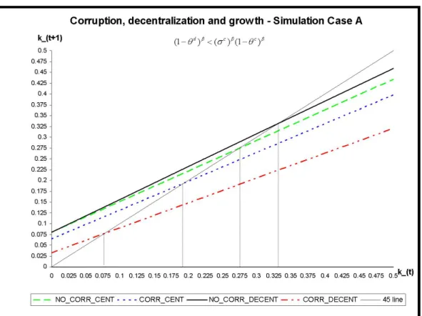
We present some simulation results in figures 2 and 3 as a way of illustrating the main results of the model. We considered standard values for the parameters and both simulations include the same parameters except for the economic effi-ciency and informational parameters. Note that regardless of the values of these, decentralisation is the best outcome in terms of development in the absence of
30Note that if mb > ng[1 +νθd(1−pδ)] then it will also be true that mb > ng. A similar
observation is valid for the other condition since ifαA(λm)α(ng)β∈(0,1)then it is also verified
thatαA(λm)α(ng)β(1−θd)β∈(0,1) .
31This can also be derived comparing equations 5.10 and 5.11. The numerator in 5.10 is
larger than the numerator in 5.11 since bothcdandngνθd(1−pδ)are both positive magnitudes. Furthermore, the denominator in 5.11 is smaller due to the presence of the term(1−θd)β.
Figure 2: Decentralisation, corruption and development. Parameter values:
α = 0.4, A = 3, λ = 1, m = 0.6, n = 0.2, g = 1.4, b = 0.6, ν = 0.3, p = 0.5,
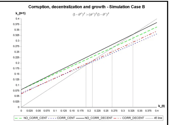
Figure 3: Decentralisation, corruption and development. Parameter values:
α = 0.4, A = 3, λ = 1, m = 0.6, n = 0.2, g = 1.4, b = 0.6, ν = 0.3, p = 0.5,
corruption. However, if corruption is present in the economy, then the outcome is ambiguous. In figure 2, where the informational differences between centralised and decentralised structures are significant (θd is significantly larger than θc), condition 5.12 is satisfied and a decentralised structure is associated to very low capital levels and indeed lower than those that would be achieved in a centralised structure. If however, the informational differences between centralised and de-centralised structures are not very important (θd is slightly larger than θc), then it can be seen in figure 3that decentralisation is associated to higher capital levels than centralisation. In fact, while our model predicts than in the absence of cor-ruption, decentralisation is the better outcome for development, we can no longer be certain that decentralisation is the better outcome if corruption is pervasive.
6
Conclusions
Decentralisation of public finance and governance has been advocated in recent decades by international organizations and national governments. Based on effi-ciency grounds, the idea that bringing the government closer to the people would result in a better and more efficient outcome yielding greater social welfare has been a strong motivation to decentralise. The traditional theory of fiscal feder-alism has been centred around this idea. The public choice literature considered the role of public agents as utility maximizers and derived slightly different impli-cations regarding the effects of decentralisation. More recently, the "new" theory of fiscal federalism is characterised by the consideration of political processes and the behaviour of public agents and the role of asymmetric information between different agents. All these theoretical considerations have introduced additional complexities to the question of whether to centralise or decentralise different gov-ernment activities. In particular, it seems that the trade-off is between efficiency-enhancing considerations stemming from the traditional theory of fiscal federalism and accountability, information and incentives stemming from the recent politi-cal economy of fispoliti-cal federalism. The issue is certainly more complex than it was originally considered and there are several interrelationships between the economic and political aspects involved.
been to provide a framework that enables us to capture some of these ideas. Our study is an attempt to contribute to the analysis of fiscal federalism and develop-ment in the presence of bureaucratic corruption. We elaborate a dynamic growth model where corruption is endogenously determined according to the decisions of individuals (in particular, public servants). In this context, the existence of a centralised or decentralised structure yield different implications in terms of the effects on economic development. Among the results of our analysis, in line with previous research on corruption and development, is that corruption is always adverse to economic development. This is because corruption diverts public re-sources away from productive activities. Furthermore, our model suggests that if corruption is absent in the economy, decentralisation is associated with greater capital accumulation than centralisation. However, if corruption occurs, then we show that decentralisation may be the worst alternative if there are weak institu-tions at the local level. This is the case if monitoring is significantly more efficient at the central level than at the local level and if the net efficiency gains associated to decentralisation are not significantly large. Finally, our model contemplates the coexistence of corruption and poverty as permanent rather than temporary features of an economy.
Our results are in accord with some results in the empirical literature. There is agreement that corruption affects economic development negatively via the di-version of investible resources. Likewise, there is agreement that corruption is also affected negatively by economic development. In fact, the new directions in empirical research conform to the hypothesis of a bivariate relationship between corruption and development. Furthermore, there is mixed evidence regarding the relationship between decentralisation and corruption in the empirical literature. While there are some studies that find that federalism is associated to more cor-ruption in the economy, other authors have found that fiscal decentralisation is associated to lower corruption. Again, the latest empirical developments suggest that it is perhaps more convenient to adopt a more integrated approach to the study of decentralisation and corruption considering the interrelationships between different aspects or types of decentralisation. The ideas presented in this chapter accord with this if we consider that improved economic efficiency is associated to certain type of decentralisation and reduced hierarchical control and informational and monitoring problems are associated to other types of decentralisation.
We think it would be desirable to pursue certain extensions to this analysis. The decision to centralise or decentralise is rarely exogenous. It may be dependent on certain features of the socio-economic system or may be part of a larger restruc-turing of the public sector. In terms of our model, this would imply to postulate that the degree of decentralisation is a function of the aggregate level of corrup-tion or development or both. Another refinement we may consider is making the probability of detection endogenous. It is likely that more efficient (costly) monitoring leads to a increase in the probability of detection. Finally, it may be important to consider the role of office-motivated politicians by incorporating national and local elections into the model. This is likely to pit the objectives of the bureaucrats against those of the politicians, with one possible effect being that local politicians may be more interested in monitoring local bureaucrats more efficiently. This would possibly reduce the ability of local bureaucrats to embezzle bureaucrats funds and alleviate local accountability problems.
References
Acemoglu, D. and Verdier, T. (1998). Property rigths, corruption and the allo-cation of talent: a general equilibrium approach,Economic Journal108: 1381– 1403.
Aghion, P. and Tirole, J. (1997). Formal and real authority in organizations,
Journal of Political Economy105(1): 1–29.
Aidt, T., Dutta, J. and Sena, V. (2005). Growth, governance and corruption in the presence of threshold effects: Theory and evidence, Cambridge Working Papers in Economics 0540, Faculty of Economics (formerly DAE), University of Cambridge.
Aidt, T. S. (2003). Economic analysis of corruption: A survey, Economic Journal 113(491): F632–F652.
Akai, N. and Sakata, M. (2002). Fiscal decentralization contributes to economic growth: evidence from state-level cross-section data for the united states, Jour-nal of Urban Economics52(1): 93–108.
Alesina, A. and Tabellini, G. (2004). Bureaucrats or politicians?, NBER Working Papers 10241, National Bureau of Economic Research, Inc.
Bac, M. (1996). Corruption, supervision, and the structure of hierarchies, Journal of Law, Economics and Organization12(2): 277–98.
Banerjee, A. (1997). A theory of misgovernance, Quarterly Journal of Economics 112(4): 1289–1332.
Bardhan, P. (1997). Corruption and development: A review of issues, Journal of Economic Literature 35(3): 1320–1346.
Bardhan, P. (2002). Decentralization of governance and development, Journal of Economic Perspectives 16(4): 185–205.
Bardhan, P. and Mookherjee, D. (2000). Capture and governance at local and national levels, American Economic Review 90(2): 135–139.
Barro, R. J. (1990). Government spending in a simple model of endogenous growth,
Journal of Political Economy98: S103–S125.
Besley, T. and Case, A. (1995). Incumbent behavior: Vote-seeking, tax-setting, and yardstick competition, American Economic Review 85(1): 25–45.
Bird, R. (1994). Decentralizing infrastructure : for good or ill?, Policy Research Working Paper Series 1258, The World Bank.
Blackburn, K., Bose, N. and Haque, E. M. (2006). The incidence and persistence of corruption in economic development, Journal of Economic Dynamics and Control 30(12): 2447–2467.
Blackburn, K. and Forgues-Puccio, G. F. (2006). Financial liberalisation, bu-reaucratic corruption and economic, Proceedings of the German Development Economics Conference, Berlin 2006 8, Verein für Socialpolitik, Research Com-mittee Development Economics.
Blanchard, O. and Shleifer, A. (2001). Federalism with and without political centralization: China versus russia,IMF Staff Papers 48(4): 8.
Brueckner, J. K. (2006). Fiscal federalism and economic growth,Journal of Public Economics90(10-11): 2107–2120.
Brunetti, A. (1997). Political variables in cross-country growth analysis, Journal of Economic Surveys11(2): 163–190.
Carbonara, E. (1998). Bureaucracy, corruption and decentralization, Working Papers 342, Dipartimento Scienze Economiche, Università di Bologna.
Davoodi, H. and Zou, H.-f. (1998). Fiscal decentralization and economic growth: A cross-country study, Journal of Urban Economics43(2): 244–257.
Di Gropello, E. (2004). Education decentralization and accountability relation-ships in latin america,Policy Research Working Paper Series 3453, The World Bank.
Ehrlich, I. and Lui, F. T. (1999). Bureaucratic corruption and endogenous eco-nomic growth,Journal of Political Economy 107(S6): S270–29.
Ellis, O. C. and Dincer, C. J. (2004). Corruption, decentralization and yardstick competition. Unpublished manuscript.
Haque, E. M. and Kneller, R. A. (2004). Corruption clubs: Endogenous thresholds in corruption and development, GEP Research Paper 2004/31, GEP Research Paper.
Hines, J. R. J. (1995). Forbidden payment: Foreign bribery and american busi-ness after 1977, NBER Working Papers 5266, National Bureau of Economic Research, Inc.
Jain, A. K. (2001). Corruption: A review,Journal of Economic Surveys15(1): 71– 121.
Kaufmann, D., Kraay, A. and Zoido-Lobaton, P. (1999). Aggregating governance indicators,Policy Research Working Paper Series 2195, The World Bank. Leach, S., Stewart, J. and Walsh, K. (1994). The changingorganisation and
man-agement of local government, Government Beyond the Centre, Palgrave McMil-lan, Basingstoke, Hampshire.
Lin, J. and Liu, Z. (200). Fiscal decentralization and economic growth in china,
Economic Development and Cultural Change49: 1–21.
Manor, J. (1999). The political economy of democratic decentralization, World Bank.
Mauro, P. (1995). Corruption and growth, Quarterly Journal of Economics 110(3): 681–712.
Mauro, P. (2004). The persistence of corruption and slow economic growth, IMF Staff Papers 51(1): 1.
Mendez, F. and Sepulveda, F. (2006). Corruption, growth and political regimes: Cross country evidence,European Journal of Political Economy 22(1): 82–98. Murphy, K. M., Shleifer, A. and Vishny, R. W. (1993). Why is rent-seeking so
costly to growth?, The American Economic Review83(2): 409–414.
Murphy, K., Shleifer, A. and Vishny, R. (1991). The allocation of talent: Impli-cations for growth, Quarterly Journal of Economics106: 503–530.
Oates, W. (2005). Toward a second-generation theory of fiscal federalism, Inter-national Tax and Public Finance 12(4): 349–373.
Oates, W. E. (1972). Fiscal federalism, New York: Harcourt Brace Jovanovich. Oates, W. E. (1999). An essay on fiscal federalism,Journal of Economic Literature
37(3): 1120–1149.
Peters, B. G. (2001). The politics of bureaucracy, fifth edition edn, Routledge, London and New York.
Prud’homme, R. (1994). On the dangers of decentralization, Policy Research Working Paper Series 1252, The World Bank.
Prud’homme, R. (1995). The dangers of decentralization, The World Bank Re-search Observer10(2): 201–220.
Rodriguez-Pose, A. and Gill, N. (2003). The global trend towards devolution and its implications, Environment and Planning C: Government and Policy 21(3): 333–351.