Stock Market Simulation

(1)

Worcester Polytechnic Institute

Digital WPI

Interactive Qualifying Projects (All Years) Interactive Qualifying Projects

February 2016

Stock Market Simulation

Yu-sen Wu

Worcester Polytechnic Institute Yulun He

Worcester Polytechnic Institute Zhijie Wang

Worcester Polytechnic Institute

Follow this and additional works at:https://digitalcommons.wpi.edu/iqp-all

This Unrestricted is brought to you for free and open access by the Interactive Qualifying Projects at Digital WPI. It has been accepted for inclusion in Interactive Qualifying Projects (All Years) by an authorized administrator of Digital WPI. For more information, please [email protected].

Repository Citation

(2)

Project Number: DZT1506

An Interactive Qualifying Project Report: Submitted to the Faculty of WORCESTER POLYTECHNIC INSTITUTE

in partial fulfillment of the requirements for the Degree of Bachelor of Science

By Yulun He ___________________________ Yu-sen Wu ___________________________ Zhijie Wang ___________________________ Submitted: February 20, 2016

Approved by Professor Dalin Tang, Project Advisor

(3)

i

Abstract

In this Interactive Qualifying Project (IQP), the group conducted a 14-week stock market simulation using three different trading strategies: technical, swing, and position trading. The team researched the fundamentals of the stock market and the basics of trading using tools and resources gathered from the Internet. Each member managed a portfolio using one trading strategy with an initial $500,000 to invest. Trading decisions were supported by market analysis techniques and results were exchanged in weekly conventions. The overall performances for the three portfolios were: technical trading: +3.86%, swing trading: +16.83%, and position trading: +13.82%. The project gave the team members a valuable beginning stock trading experience and helped them to gain a better knowledge and understanding of the stock market. This IQP has built a strong foundation for potential investment in the future.

(4)

ii

List of Figures

Figure 1.5.1. Moving Average [12] ... 8

Figure 1.5.2. RSI Indicator Chart [13] ... 9

Figure 1.5.3. Bollinger Bands: EXXON Prices [39] ... 10

Figure 2.2.1. Sample Trend Line Trading Method [19] ... 15

Figure 2.3.1. The historical sale resulted in a net gain of 78% in nine months [21] ... 16

Figure 2.4.1. Simulation Program Interface... 18

Figure 2.4.2. Edit/Delete Holdings Details ... 18

Figure 2.4.3. Chart in Yahoo Simulator ... 19

Figure 3.4.1. AMZN Behavior during the Preparation Week... 71

Figure 3.5.1. Amazon's history performance ... 26

Figure 3.5.2. Tesla's history performance ... 26

Figure 3.5.3. JP Morgan's 5-year performance ... 27

Figure 3.5.4. Exxon Mobil 5-year performance ... 28

Figure 3.5.5. IHG history performance ... 29

Figure 4.1.1. Yahoo AMZN Sept 4 – Oct 2 ... 30

Figure 4.1.2. Yahoo OPGN share price Sept 18 – Oct 2 ... 31

Figure 4.1.3. Yahoo INTEL Sept 18 – Oct 2 ... 31

Figure 4.2.1. Yahoo TSLA Oct 2 – Oct 10 ... 33

Figure 4.2.2. Yahoo INTEL & MSFT Oct 2 – Oct 10 ... 34

Figure 4.3.1. Matlab TSLA Jul 1 – Oct 18 ... 36

Figure 4.3.2. Matlab AMZN Jul 1 – Oct 18... 37

Figure 4.4.1. Matlab ACE Jul 1 – Oct 23 ... 40

Figure 4.4.2. Matlab TRC Jul 1 – Oct 23... 41

Figure 4.5.1. Matlab SMP Jul 1 - Oct 30 ... 43

Figure 4.5.2. Matlab ASR Jul 1 - Oct 30 ... 44

Figure 4.6.1. Matlab UTL Jul 1 - Nov 6 ... 46

Figure 4.7.1. Matlab HSY Jul 1 - Nov 13 ... 48

Figure 4.7.2. Matlab MDC Jul 1 - Nov 13 ... 48

Figure 4.8.1. Matlab BR Aug 1 - Nov 20 ... 51

Figure 4.8.2. Matlab SFE Aug 1 - Nov 20 ... 51

Figure 4.9.1. Matlab AIZ Aug 1 - Nov 27 ... 54

Figure 4.9.2. Matlab FFG Aug 1 - Nov 27 ... 55

Figure 4.10.1. Matlab CUZ Aug 1 - Dec 4 ... 57

Figure 4.10.2. Matlab PGEM Aug 1 - Dec 4 ... 58

Figure 4.11.1. Yahoo Dow Dec 6 - Dec 11 ... 60

Figure 4.11.2. Yahoo Nasdaq Dec 6 - Dec 11 ... 60

Figure 4.11.3. Yahoo S&P 500 Dec 6 - Dec 11 ... 61

Figure 4.12.1. Matlab NSP Sep 1 - Dec 18 ... 63

Figure 4.12.2. Matlab BMY Sep 1 - Dec 18 ... 64

Figure 4.14.1. Matlab CPAC Sep 1 - Dec 31... 67

Figure 4.14.2. Matlab TRP Sep 1 - Dec 31 ... 68

Figure 4.14.3. Matlab PSA Sep 1 - Dec 31 ... 69

Figure 5.1.1. Week 1 Performance of BIDU Sep. 28 – Oct. 2 ... 73

(8)

vi

Figure 5.1.3. Week 1 Performance of VOW3.DE Sep. 28 – Oct. 2 ... 75

Figure 5.1.4. Week 1 Performance of AUDI Sep. 28 – Oct. 2 ... 75

Figure 5.2.1. Week 2 Performance of APPL Oct. 5 – Oct. 9 ... 78

Figure 5.2.2. CVX Performance of 2015 ... 78

Figure 5.3.1. Week 3 Performance of AAPL Oct. 12 – Oct. 16 ... 79

Figure 5.4.1. Week 4 Performance of CBI Oct. 19 – Oct. 23 ... 81

Figure 5.5.1. 3-Month Performance of GoPro Jul. 29 – Oct. 28 ... 83

Figure 5.5.2. 1-Month Performance of Walmart Sep. 29 – Oct. 28 ... 83

Figure 5.5.3. 1-Month Performance of KO Sep. 29 – Oct. 28 ... 84

Figure 5.6.1. 1-Month Performance of KO Oct. 4 – Nov. 3 ... 85

Figure 5.6.2. 1-Month Performance of ROBO Oct. 4 – Nov. 3 ... 86

Figure 5.7.1. 1-Month Performance of AIXG Oct. 14 – Nov. 13 ... 88

Figure 5.7.2. 1-Month Performance of IHG Oct. 14 – Nov. 13 ... 88

Figure 5.7.3. 1-Month Performance of YOKU Oct. 14 – Nov. 13 ... 89

Figure 5.8.1. 1-Month Performance of AIXG Oct. 21 – Nov. 20 ... 91

Figure 5.8.2. 1-Month Performance of AR Oct. 19 – Nov. 18 ... 91

Figure 5.8.3. 1-Month Performance of FORD Oct. 19 – Nov. 18 ... 92

Figure 5.8.4. 1-Month Performance of SPWR Oct. 19 – Nov. 18 ... 92

Figure 5.9.1. Performance of BBY Nov. 19 - Nov. 27 ... 94

Figure 5.9.2. 1-Month Performance of WMT Oct. 28 - Nov. 27... 95

Figure 5.9.3. One-Month Performance of NFLX Aug. 28 - Nov. 27 ... 95

Figure 5.9.4. One-Month Performance of AAPL Oct. 28 - Nov. 27 ... 96

Figure 5.10.1. 3-Month Performance of AMZN Sep. 8 – Dec. 5 ... 97

Figure 5.10.2. 1-Month Performance of NFLX Nov. 5 – Dec. 4... 98

Figure 5.10.3. 1-Month Performance of ATVI Nov. 5 - Dec. 4 ... 98

Figure 5.10.4. 1-Month Performance of WMT Nov. 5 - Dec. 4 ... 99

Figure 5.10.5. 1-Month Performance of KR Nov. 5 - Dec. 4 ... 100

Figure 5.10.6. 1-Month Performance of AIXG Nov. 5 - Dec. 4 ... 100

Figure 5.11.1. 1-Month Performance of NFLX Nov. 8 – Dec. 7... 101

Figure 5.11.2. 1-Month Performance of FSLR Nov. 9 – Dec. 8 ... 102

Figure 5.11.3. 1-Month Performance of WMT Nov. 10 – Dec. 9 ... 103

Figure 5.11.4. 1-Month Performance of KR Nov. 10 – Dec. 9 ... 103

Figure 5.11.5. 1-Month Performance of AIXG Nov. 10 – Dec. 9 ... 104

Figure 5.11.6. 1-Month Performance of ATVI Nov. 11 – Dec. 10 ... 105

Figure 5.11.8. 1-Month Performance of YUME Nov. 11 – Dec. 10 ... 106

Figure 5.12.1. 1-Month Performance of SUNE Nov. 15 – Dec. 14... 107

Figure 5.12.2. 1-Month Performance of BAC Nov. 16 – Dec. 15 ... 107

Figure 5.12.4. 1-Month Performance of FNSR Nov. 17 – Dec. 16 ... 108

Figure 5.12.5. 1-Month Performance of AMAT Nov. 19 – Dec. 18 ... 109

Figure 5.12.6. 1-Month Performance of KANG Nov. 19 – Dec. 18 ... 109

Figure 5.13.1. 1-Month Performance of FSLR Nov. 22 – Dec. 21 ... 111

Figure 5.13.2. 1-Month Performance of WMT Nov. 23 – Dec. 22 ... 111

Figure 5.13.3. 1-Month Performance of BAC Nov. 24 – Dec. 23 ... 112

(9)

vii

Figure 5.14.1. 1-Month Performance of SUNE Nov. 29 – Dec. 28... 114

Figure 5.14.2. 1-Month Performance of AMAT Nov. 30 – Dec. 29 ... 115

Figure 5.14.3. 1-Month Performance of GE Dec. 1 – Dec. 30 ... 115

Figure 5.14.4. 1-Month Performance of FSLR Dec. 1 – Dec. 30 ... 116

Figure 5.14.5. 1-Month Performance of WMT Dec. 1 – Dec. 30 ... 116

Figure 5.14.6. 1-Month Performance of KANG Dec. 2 – Dec. 31 ... 117

Figure 5.14.7. 1-Month Performance of FNSR Dec. 2 – Dec. 31 ... 117

Figure 6.1.1. Week 1 S&P 500 Performance (Sep. 28 – Oct. 2) ... 121

Figure 6.1.2. Week 1 Dow Jones Performance (Sep. 28 – Oct. 2) ... 122

Figure 6.1.3. Week 1 Performance of Exxon Mobil (Sep. 28 – Oct. 2) ... 123

Figure 6.1.4. Week 1 Performance of Tesla Motor (Sep. 28 – Oct. 2) Week 2 ... 124

Figure 6.1.5. Week 1 Amazon Performance (Sep. 28 – Oct. 2) ... 124

Figure 6.2.1. Week 2 Performance for S&P 500 (Oct. 5 – Oct. 9) ... 126

Figure 6.2.2. Week 2 Performance for Tesla Motors (Oct. 5 – Oct. 9) ... 127

Figure 6.2.3. Week 2 Performance for General Electric (Oct. 5 – Oct. 9) ... 127

Figure 6.2.4. Week 2 Performance for Amazon (Oct. 5 – Oct. 9) ... 128

Figure 6.3.1. Week 3 Performance for Dow Jones Index (Oct. 12 – Oct. 16) ... 129

Figure 6.3.2. Week 3 Performance for NASDAQ (Oct. 12 – Oct. 16) ... 130

Figure 6.4.1. Week 4 Performance for NASDAQ Index (Oct. 19 – Oct. 23) ... 131

Figure 6.4.2. Week 4 Performance for Dow Jones (Oct. 19 – Oct. 23) ... 132

Figure 6.4.4. Week 4 Performance for Boeing (Oct. 19 – Oct. 23) ... 133

Figure 6.5.2. Week 5 Performance for IHG (Oct. 26 – Oct. 30) ... 136

Figure 6.6.1. Week 6 Performance for Amazon (Nov. 2 – Nov. 6) ... 137

Figure 6.6.2. Week 6 Performance for IHG (Nov. 2 – Nov. 6) ... 138

Figure 6.7.1. Week 7 Performance of Dow Jones (Nov. 9 – Nov. 13) ... 139

Figure 6.7.2. Week 7 Performance of NASDAQ (Nov. 9 – Nov. 13) ... 140

Figure 6.7.3. Week 7 Performance of Amazon (Nov. 9 – Nov. 13) ... 141

Figure 6.8.1. Week 8 Performance for S&P 500 (Nov. 16 – Nov. 20) ... 143

Figure 6.8.2. S&P 500 Performance at 9/11/2001 ... 143

Figure 6.8.3. Week 8 Performance for Sunoco (Nov. 16 – Nov. 20) ... 144

Figure 6.8.4. Week 8 Performance for Amazon (Nov. 16 – Nov. 20) ... 145

Figure 6.9.1. Week 9 Performance of S&P Index (Nov.23 – Nov. 27) ... 146

Figure 6.9.2. Week 9 Performance for Macy's (Nov.23 – Nov. 27) ... 147

Figure 6.9.3. Week 9 Performance for Nordstrom (Nov.23 – Nov. 27) ... 148

Figure 6.9.4. 3-Month Performance for Amazon (Aug. 29 - Nov. 29) ... 149

Figure 6.10.1. Week 10 Performance for S&P500 (Nov. 30 - Dec. 4) ... 150

Figure 6.10.2. Week 10 Performance for Amazon (Nov. 30 - Dec. 4) ... 151

Figure 6.10.3. Historical Price for WTI Crude Oil [42] ... 151

Figure 6.10.4. 3-Month Performance for JP Morgan & Chase (Sep. 1 – Dec. 1)... 152

Figure 6.10.5. Week 10 Performance for JP Morgan & Chase (Nov. 30 - Dec. 4) ... 153

(10)

viii

Figure 6.11.1. Week 11 Performance of S&P 500 (Dec. 7 – Dec. 11) ... 155

Figure 6.11.2. Week 11 Performance for NASDAQ Composite (Dec. 7 – Dec. 11) ... 156

Figure 6.11.3. Week 11 Performance for Amazon (Dec. 7 – Dec. 11) ... 157

Figure 6.11.4. Week 11 Performance for ExxonMobil (Dec. 7 – Dec. 11) ... 158

Figure 6.11.5. Week 11 Performance for JP Morgan (Dec. 7 – Dec. 11) ... 158

Figure 6.12.1. . Week 12 Performance for S&P500 (Dec. 14 - Dec. 18) ... 160

Figure 6.12.2. Week 12 Performance for Amazon (Dec. 14 - Dec. 18) ... 160

Figure 6.13.1. Week 13 Performance for S&P500 (Dec 21 - Dec. 24) ... 161

Figure 6.13.2. Week 13 Performance for Amazon (Dec 21 - Dec. 24) ... 162

Figure 6.13.3. Week 13 Performance for Wal-Mart (Dec 21 - Dec. 24) ... 162

Figure 6.14.1. Week 14 Performance for Amazon (Dec. 28 - Dec. 31) ... 164

Figure 7.1.1. Technical Trading Profit/Loss for Each Company ... 165

Figure 7.1.2. Swing Trading: Profit/Loss for Each Company ... 167

Figure 7.1.3. Position Trading: Total Profit/Loss for Each Company ... 168

Figure 7.1.4. Amazon Performance for 6 month showing major transactions ... 169

(11)

ix

List of Tables

Table 1.4.1. The composition of Dow Jones ... 5

Table 1.5.1. A typical stock table ... 7

Table 3.2.1. Quarterly Balance Sheet for Amazon [23] ... 21

Table 4.1.1. Transactions for Week 1 ... 32

Table 4.2.1. Transactions Week 2 ... 35

Table 4.3.1. Transactions for Week 3 Algorithm 1 ... 39

Table 4.7.1. Transactions for Week 7 Algorithm 2 (Potential Loss) ... 47

Table 5.1.1. Transaction Sheet for Week 1 Sep. 21 – Sep. 25 ... 72

Table 5.4.1. Transaction Sheet for Week 4 Oct. 19 – Oct. 23 ... 81

Table 5.5.1. Transaction Sheet for Week 5 Oct. 26 – Oct. 30 ... 84

Table 5.6.1. Transaction Sheet for Week 6 Nov. 2 – Nov. 6 ... 87

Table 5.10.1. Transaction Sheet of Week 10 Nov. 30 – Dec. 4 ... 101

Table 5.11.1. Transaction Sheet of Week 11 Dec. 7 – Dec. 11 ... 106

Table 6.1.1. Transaction Sheet for Week 1 (Sep. 28 – Oct. 2) ... 119

Table 6.2.1. Transection Sheet for Week 2 (Oct. 5 – Oct. 9) ... 125

Table 6.5.1. Transaction Sheet for week 5 (Oct. 26 – Oct. 30) ... 134

Table 6.7.1. Transaction Sheet for Week 7 (Nov. 9 – Nov. 13) ... 139

Table 6.8.1. Transaction Sheet for Week 8 (Nov. 16 – Nov. 20) ... 142

Table 6.9.1. Transaction Sheet for Week 9 (Nov.23 – Nov. 27) ... 146

Table 6.10.1. Transaction Sheet for Week 10 (Nov. 30 – Dec. 4) ... 149

Table 6.11.1. Transaction Table for Week 11 (Dec. 7 – Dec. 11) ... 154

(12)

1

1. Introduction

1.1 Goal

The objective of this IQP is to become competent in the field of investment in the stock market by researching the fundamentals and acquiring a solid understanding of the strategies and skills essential to become successful investors. It is imperative that we dedicate a significant portion of this project to accumulating information before investing. We will spend the first 7 weeks exploring various topics regarding background information of the stock market. During this time, we will also need to familiarize ourselves with the terminology and learn to how use the tools that will provide us an interpretation of the market. After building a foundation, we will then apply the newfound knowledge by means of a stock market simulation. In each simulation, a different strategy will be utilized such that we can compare progress. At the end of the simulation, we will assess the overall results and try to understand cause and effect. As a result of the simulation, we hope to take away useful skills that will help us become better investors as well as to have an open mind for the market.

1.2 History of the Stock Market

The early beginnings of the stock market dates back hundreds of years ago as a simple form of money lending where these “lenders” traded debts amongst themselves. In exchange for high-risk, profit could be made from these high-interest loans. As this business grew, the lenders began selling these debts to other people.

The first people to make significant advance in this field were Venetians who traded securities from other governments. They carried on this practice which can be dated back to the 1300s.

(13)

2 The first stock exchange was established in Antwerp, Belgium in 1531 where moneylenders and other parties of interest would come together to do business and resolve other ordeals. This establishment dealt with more of financial partnerships rather than trading “stocks”. We can see that the beginnings of the stock market first starts with a sense of trust and relationship building to produce profitable returns.

Around a century later, East India and Asia were highly profitable areas of trade for the Dutch, British, and French governments. However, the issue with the trades stems from the physical transfer of the goods itself. The voyages required to transport the goods involved great risk influenced by a variety of factors. Ship owners sought investors for the sake of not losing all their profit if their ship were lost. If the trade was successful, investors would receive a percentage of the profit having provided some provision. This collective investment is an early example of a joint stock company.

One company that emerged with government aid was the British East India Company. Since investors wanted a piece of the profit, competition rose. As a result, the financial market experienced great change. Another company, the South Seas Company had a similar system backed by the king in which investors bought shares immediately when they were issued. The problem with this mindset is that shares that did not make sense or have reason could easily be slipped in and bought. The end result was the South Seas Company crashing.

The New York Stock Exchange, formed by a group of brokers in 1792, became the center of business and trade in the United States. It quickly rose to become a power stock exchange center both in the US and outside. In 1971, with the advance of technology, NASDAQ became a competitor as a result of electronic trades which were more efficient [1].

(14)

3

1.3 Factors Influencing Stock Market

The stock price, also known as share price or market price, is the current cost of purchasing a security on an exchange of equity of an asset or service and is essentially determined by the most recent price at which the stock was traded [2].

Similar to everyday commodity prices, stock prices vary from time to time yet with a significantly larger degree of fluctuation. This fundamental behavior of stock prices is a reflection of supply and demand. When prospective buyers outnumber sellers, demand becomes too high and subsequently the stock price rises. On the other hand, when sellers outnumber buyers, supply takes the lead and thus the stock price falls [3]. If more investors want a stock and are willing to pay more, the stock price will go up. If more investors are selling a stock and there appears to be a lack of buyers, the stock price will go down [4]. The factors that drive such behaviors of investors are the fundamental causes of the volatility of the stock prices. The stock market is difficult to predict due to the enormous number of potential factors. A good comprehension of such factors is necessary for basic stock trading [5].

One of the major factors that affect the value of a company is its own performance. The performance can be determined by the company’s report history, future estimated earnings, announcement of dividends, introduction of a new product or a product recall, takeover or merger, change of employment, etc. For instance, earnings are major measurements of the companies’ performances. Public companies are required to report their earnings once each quarter of the year and during these earning seasons investors determine the future value of the companies. Therefore, decisions are made based on their analysis of the earnings projection.

The performance of the company itself certainly is not the only factor that changes the stock price. The performance of the whole industry can also play a major part in the fluctuation

(15)

4 of the market. Often, the stock price of the companies in the same industry will move in the same direction with each other because market conditions generally have similar effect on the companies in the same industry. If industry A has the tendency to replace industry B, most likely the stock prices of A will increase and those of B will decrease.

Investor sentiment can also influence the stock prices. If investors are positive and confident towards the market, the market is likely to become a bull market that makes the stock prices go up. Accordingly, if investors hold negative expectations and fading confidence towards the market, it becomes a bear market and stock prices fall.

The last main factor on stock price is the big economic environment. This includes interest rates, governmental policies, inflation/deflation, and value of the country’s currency, etc. For example, if the interest rates increase when a company owes money to the bank, its liability also increases since it has to pay more on interest. Therefore, the company may reduce the profit and dividends it pays the shareholders. As a result, the company loses shareholders and the stock price drops. Another example is the governmental policies. If certain newly enacted policies benefit certain industries the stock price of these industries will increase. This also relates to the performance of the industry as discussed above [6].

1.4 Stock Market Index

Stock market index is a powerful tool to measure the value of a section of the stock market. Learning how to analyze the stock market indices will help us understand the trends in the stock market. Therefore, it is a critical component for our project. Stock market indices are usually computed from prices of selected stocks. They may be classified by region. The global index includes MSCI World and S&P Global 100. Some regional indices include the American S&P 500, the Japanese Nikkei 225, and the British FTSE 100. Since our project stimulates the

(16)

5 stocks in the U.S. Market, we will focus on American stock market indices. There are three major stock indices in the U.S.: Dow Jones Industrial Average, NASDAQ Composite and S&P 500.

1.4.1 Dow Jones Industrial Average

The Dow Jones Industrial Average, the second oldest U.S. market index, also called the Dow Jones, is created by Wall Street Journal editor and Dow Jones & Company. “It is an index that shows how 30 large publicly owned companies based in the U.S. have traded during a standard trading session in the stock market. The average is price-weighted, and to compensate for the effects of stock splits and other adjustments, it is currently a scaled average" [7].

Only few best U.S. companies can be selected as a Dow Jones’s company. Some standards for Dow Jones’s selection include the excellent reputation, sustained growth, and interest to a large number of investors. As of September 4th_{2015, the composition of Dow Jones}

is shown in Table 1.4.1.

Table 1.4.1. The composition of Dow Jones

Apple Inc. The Home Depot, Inc. NIKE, Inc.

American Express Company International Business Machines

Corporation Pfizer Inc.

The Boeing Company Intel Corporation The Procter & Gamble Company

Caterpillar Inc. Johnson & Johnson The Travelers Companies, Inc.

Cisco Systems, Inc. JPMorgan Chase & Co. UnitedHealth Group Incorporated Chevron Corporation The Coca-Cola Company United Technologies

Corporation E. I. du Pont de Nemours and

Company McDonald's Corp. Visa Inc.

The Walt Disney Company 3M Company Verizon Communications

Inc.

General Electric Company Merck & Co. Inc. Wal-Mart Stores Inc. The Goldman Sachs Group,

(17)

6 1.4.2 NASDAQ Composite

Along with the Dow Jones Industrial Average and S&P 500, NASDQ is one of the three most-followed indices in U.S. stock market. The composition of the NASDAQ Composite is heavily weighted towards information technology companies. As of 24 April 2015, NASDAQ composite’s component had 5073 companies [8].

1.4.3 Standard & Poor’s 500

S&P 500 is based on the market capitalization of 500 leading companies having common stock listed on the NYSE or NASDAQ. S&P 500 is the most widely used U.S. market stock index because contrast to NASDAQ, it covers all important industries in the U.S. rather than only IT domain, and it contains more companies than Dow Jones which is 30 largest. Therefore, S&P 500 is famous for its diverse constituency and weighting methodology. For selection standard, S&P 500 only select U.S. companies with market cap of USD 5.3 billion or greater [9]. In the following simulation, we used S&P 500 as a major benchmark to assess the general performance of U.S. market.

1.5 Stock Market Indicators

1.5.1 Interpretation of Stock Table

Table 1.5.1 shows a typical stock table/quote that lists information regarding the details of the stock performance.

(18)

7

Table 1.5.1. A typical stock table

Columns 1 & 2 represent the highest and lowest prices that the stock has experienced in one year. Column 5 is the dividend per share which shows the annual dividend payment per share. The blanks indicate that the company does not pay out dividends. Column 6 is the dividend yield which is the percent return on the dividend. It is calculated as the quotient of the annual dividends per share and price per share. Column 8 is the volume of trade which represents the number of trades in the day in hundreds. Column 9, 10 & 11 are the day’s high, low, and close respectively. Column 12 is the net change from the previous day’s close price.

These definitions of course do not only apply to tables, but also in interpreting the graphs that visually display the same data [10].

1.5.2 Moving Averages

In mathematics, a moving average is an analysis method of interpolating the data points by carrying out series of averages of different subsets of the full data set. In the stock market, a moving average (MA) utilizes past prices of a stock to provide trend-following or lagging information of that stock that can be exploited by the investors to predict future movement of the share price. Simple moving average (SMA), average of a security over a defined number of time periods, and exponential moving average (EMA) are the two basic and commonly used MAs.

(19)

8 The most common applications of MAs are to identify the trend direction and to determine support and resistance levels [11].

MA crossover is the most basic type of signal and is favored among many stock traders as it is fairly objective. The first type of crossover is when the price of a stock moves from one side of a MA and crosses to the other side. A cross above a MA can signal the beginning of an uptrend and would likely be used by traders as a suggestion of buying and vice versa. The second type of crossover occurs when a short-term average crosses above a long-term average. This is used by traders to determine the momentum shift towards a strong behavior of the asset, similarly to the first type [12].

Figure 1.5.1 shows an example of two moving averages with different periods. As explained above, the cross between a short and long term moving average indicated a strong shift in trend which can be seen below. The price moves from a flat trend to a strong upward trend.

Figure 1.5.1. Moving Average [12]

This indicator is featured in many popular trading mediums and is a very useful tool for analysis techniques. By understanding its characteristics and how it applies to stock trends, we can use this knowledge to predict future trends and support our trading decisions.

(20)

9 1.5.3 Relative Strength Index (RSI)

The RSI values indicate when the stock is about to change in trend. RSI helps to signal overbought and oversold conditions in a security.

“The indicator is plotted in a range between zero and 100. A reading above 70 is used to suggest that a security is overbought, while a reading below 30 is used to suggest that it is oversold. This indicator helps traders to identify whether a security's price has been unreasonably pushed to current levels and whether a reversal may be on the way.” [13]

Figure 4.6.1 shows an example chart using the RSI values. When the RSI values exceed 70, stocks have been overbought and the trend changes slightly later. The same is seen when the stocks have been oversold.

Figure 1.5.2. RSI Indicator Chart [13]

One potential use for this tool is to support a decision for holding onto stocks. If the stock is currently in an uptrend and the RSI data shows that the curve is bounded by the overbought and oversold lines, then it indicates that the trend change is less likely to occur. Therefore, a trader would be more confident in holding during an uptrend. Another method would be to seek

(21)

10 out the trend changes instead. If a stock is in a downtrend and the curve goes below the oversold line in the RSI chart, then it indicates that a trend change is more likely to occur. A trader that is lucky enough predict accurately and catch the trend change would reap profit.

1.5.4 Bollinger Bands

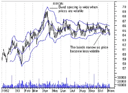
Bollinger Bands were developed by John Bollinger in the early 1980s. This tool has been regarded as a valuable means to make trading decisions by analyzing the volatility of the market. There are three bands to be considered: an upper, middle, and lower band. The middle band represents an intermediate movement of the securities prices often in the form of a moving average curve. The enveloping bands are determined by the volatility usually the standard deviation.

Figure 1.5.3 shows an example of Bollinger bands on a typical price chart. EXXON is used as the example here. It is important to note that the bands contain the prices very well.

Figure 1.5.3. Bollinger Bands: EXXON Prices [39]

The interpretation of the bands is rather simple. In short, the characteristic to monitor is the outer bands’ deviation from the middle. If the deviation is large, a high volatility (large

(22)

11 changes in price) is implied. The converse is also true that smaller deviations imply low volatility (small changes in price). Generally, security prices tend to remain within the bounds of the upper and lower bands [14].

According to Technical Analysis from A to Z by Steven B. Achelis, the following characteristics of the Bollinger Bands were noted by Mr. Bollinger himself.

• Sharp price changes tend to occur after the bands tighten, as volatility lessens. • When prices move outside the bands, a continuation of the current trend is implied.

• Bottoms and tops made outside the bands followed by bottoms and tops made inside the bands call for reversals in the trend.

• A move that originates at one band tends to go all the way to the other band. This observation is useful when projecting price targets.

(23)

12

2. Trading Methods

The goal of this project is to simulate the trading in stock market and gain experience that could be applied in real life. To achieve this goal, some common trading methods are studied, they are: position trading, swing trading, and technical trading. Each trading method was studied in the following sections and each group member selected their own trading method.

2.1 Technical Trading

“It has been observed that human nature remains more or less constant and tends to react to similar situations in consistent ways. Based on this premise, by studying the nature of previous market turning points, it is possible to develop some characteristics that can help identify major market tops and bottoms. The technical approach to investment is essentially a reflection of the idea that prices move in trends that are determined by the changing attitudes of investors towards a variety of economic, monetary, political, and psychological forces” [15].

The technique encompasses a broader spectrum of trading. It does not only apply inclusively to trading, but is applied by economists and meteorologists. The goal of this method is collect data of past trades, combine them, and produce a model that can predict future trends. These traders analyze patterns and consider hundreds of factors that can have an influence on the curves of the graphs.

The data that a technical trader must analyze is too much to review by numbers alone. Tools were created to represent the data in a visually friendly way. A chart is one representation of the data that plots useful information so that observations can be made regarding the prices relative to time.

Technical traders look for indications to find where recognizable trends are likely to occur. “A vast majority of chart patterns may be divided into two main groups: reversal and

(24)

13 continuation. Reversal patterns indicate a change in the previous trend occurring in the market. “Continuation patterns confirm the movement of market in the same direction as the previous trend” [15]. Using this logic, a critical scenario would be recognizing continuation patterns in an uptrend. Another would in the case where the prices are moving in a downtrend. With trend reversal indicators and good timing a trader can secure large profits.

Although some patterns in history may repeat themselves, it has its limitations and cannot be used to fully predict the future patterns. It provides a starting point for investors to consider as a candidate for potential trade [16]. Accurate analysis requires more experience and study in the area. A combination using technical analysis in conjunction with other techniques is more ideal. Even more, the ability to weight indications is necessary for predicting trends.

Investment Analysis and Portfolio Management provides examples and more advanced technical indicators for reference. However, this IQP will use basic indicators to analyze patterns.

2.2 Swing Trading

Swing trading is a common trading strategy that the traders use to capture gains in a stock within a short range of time, typically between one day and one or two weeks. Unlike position traders, swing traders focus more on the short-time price momentum pattern of the stocks rather than the fundamental and intrinsic factors that the stocks are related to and affected by [17].

The best candidates for swing trading are the large-cap stocks that are most actively traded on the major stock exchanges because these stocks are most likely to demonstrate clear trends within short periods of time and thus swing traders ride on the wave until they predict a new trend is going to take over the old one.

(25)

14 The best time to perform swing trading is when the market is either a strong bear or bull market and any market in between these two extremes are not considered to be good because in these two extremes the stock prices are generally carried in one direction only whereas in the regular markets the stock price tends to stay stable, which swing traders will not be able to benefit much from [18].

According to Wiley Trading: Swing and Day Trading Evolution of a Trader, two of the most commonly used techniques for swing trading are support/resistance and trend line analysis. A general rule of thumb for support and resistance is to buy at support and sell at resistance. Another way to swing trade on support and resistance is too short at resistance and cover at support. However, in this simulation, the trader will not deploy at tactics on shorting. Determining support and resistance is therefore crucial to swing trading as often times price drops much faster than it rises. One example of extrapolating the information lies in areas denoted as peaks and valleys that indicate resistance and support, respectively.

Trend line trading is a very popular technique that can be applied to swing trading, position trading, and technical trading. By definition, a trend line is a line that connects lows or the highs over to project out into the future. It is critical to select the accurate trend lines to determine the direction of the stock. The trend lines should not be broken as in they should not be intersected by some lows or highs along the lines. If this ever occurs, a new trend line should be created. On a bullish market, we want to buy a stock when the price line approaches the trend line underneath it because the stock price will most likely to curve up. Similarly, for a bearish market, we want to sell the stock when the price line reaches the overhead trend line to minimize the loss or to still profit. This can be demonstrated in Figure 2.2.1 below.

(26)

15

Figure 2.2.1. Sample Trend Line Trading Method [19]

2.3 Position Trading

Position trading is a very common method that involves long term investment. This strategy involves doing more research initially, taking a position, and then monitoring and managing it. It also is less time consuming than other trading methods due to the lower trading frequency and is not limited to any particular market. These traders view short-term fluctuations as minor since they believe that it will all even out in the future. The evaluation of the asset using this method involves understanding the charts and profit is from the move in trends [20].

Generally, the position trading can carry less risk than buy and hold. The reason for that is timing the exit can lower the chance of losses.

One of the risks of position trading is that ignoring minor fluctuations can actually turn into a disadvantage because a trend change may occur. Since the concept of position trading is based on holding stocks for long periods, position traders may fall into a trap of investing in a

(27)

16 declining market. Many of these traders have set safety lines in order to prevent themselves from that situation.

In Wiley Trading: Fundamental Analysis and Position trading: Evolution of a Trader, the author indicates a typical pattern of stock performance as shown in Figure 2.3.1, which is called a high-and-tight flag. It means when the price of a stock rises by at least 90 percent, a flag pattern usually appear, which is often a good signal to invest in the stock. Usually the move up will be replicated when the stock leaves the flag zone [21].

Figure 2.3.1. The historical sale resulted in a net gain of 78% in nine months [21]

A beginner to the positon trading should pay attention to the news of the stock market. News usually has great impact on a specific stock price as well as general market trends. The author of the book considers news as a key factor to predict when the indexes will transition

(28)

17 from bull to bear or the reverse. For example, if the market is at bottom and bad news does not push the index lower and good news encourage the market to go up, then this would imply that the markets are ready to go higher [21].

Another lesson from the book is that beginner of position trading should focusing more on the primary price trends as the phrase saying, go with the flow and rising tide lifts all boat. The stock in bull market usually outperformed the similar company in bear market. Although this may sound obvious but is helpful for the beginner [21].

Because the simulation will last only 14 weeks, stocks will be traded with a higher frequency than normal position trader who can hold a stock for months or years. However, it will still be a lower frequency compared to swing trading. Therefore, a distinction can be made to compare the methods at the end of the simulation.

2.4 Simulation Program

There are many simulation programs available on the internet, such as Investopedia and StockTrak. The program the group will be using is Yahoo Finance, because it integrates many functions actual trading applications provide. It allows users access to real-time information and investment updates to stay on top of the market. It even goes beyond stocks and track currencies, commodities and more. It is also convenient to choose Yahoo Finance because it has a default application on mobile phones which makes it easy to monitor the market information anytime and anywhere.

The interface of the simulation program is shown in Figure 2.4.1. There are many different functions that can be turned on or off display. Some of the useful ones that will be used will be GAIN & % GAIN which will give us an idea roughly of the earnings and losses.

(29)

18

Figure 2.4.1. Simulation Program Interface

To buy or sell a stock we can use the Add/edit holdings function as shown in Figure 2.4.2, to buy a stock, first, we entered the number of shares, and entered the price paid for each share. We can also enter the cost for each commission, but we assumed commission is 0 for trading.

Figure 2.4.2. Edit/Delete Holdings Details

We can also find the history chart and static information in “Chart, News, Stats, Options, Board” function as shown in Figure 2.4.3. This opens up an interactive chart which implements many different features such as moving averages, RSI, and Bollinger Bands. Using this tool will be necessary when we make trades.

(30)

19

(31)

20

3. Company Selections

Before buying a company’s stock, the investors usually evaluate the stock by its valuation, strategy, plans for diversification and appetite for risk. After considering these factors, each group member chose ten stocks that will be potential candidates for investment in this project.

3.1 Price-Earnings Ratio (P/E)

The price earnings ratio, also called P/E ratio, is an indicator to determine whether a stock is suitable to buy at a certain time. It is determined by the company’s market value and investors’ expectation for the company. The smaller the P/E ratio means you would claim more than what you pay. So usually investor will seek the stock with lower P/E ratio. But sometimes high P/E ratio does not automatically mean that the company would be a bad investment because it might have an expected growth in the future. The Price-Earnings Ratio is calculated from following equation:

𝑃𝑃𝑃𝑃𝑃𝑃𝑃𝑃𝑃𝑃

𝐸𝐸𝐸𝐸𝑃𝑃𝐸𝐸𝑃𝑃𝐸𝐸𝐸𝐸𝐸𝐸

𝑅𝑅𝐸𝐸𝑅𝑅𝑃𝑃𝑅𝑅

=

𝑀𝑀𝑀𝑀𝑀𝑀𝑀𝑀𝑀𝑀𝑀𝑀_{𝐸𝐸𝑀𝑀𝑀𝑀𝐸𝐸𝐸𝐸𝐸𝐸𝐸𝐸𝐸𝐸}𝑉𝑉𝑀𝑀𝑉𝑉𝑉𝑉𝑀𝑀_{𝑝𝑝𝑀𝑀𝑀𝑀}𝑝𝑝𝑀𝑀𝑀𝑀_{𝑆𝑆ℎ𝑀𝑀𝑀𝑀𝑀𝑀}𝑆𝑆ℎ𝑀𝑀𝑀𝑀𝑀𝑀

(1) The price earning is a critical indicator reflects a company’s potential to grow and gain more profit. The team took P/E ratio in consideration during company selection [22].

3.2 Financial Statement

There are three major financial statements available: Income statement, Balance sheet and Cash flow. Among those three, we focused more on the balance sheet because it tells the financial state of a company.

Balance sheet is the statement of company’s assets, liabilities, and capital at a certain point of time. It provides the balance of income and expenditure over the preceding period. Table 3.2.1 is one example of typical balance sheet. It provides us three critical financial pieces of

(32)

21 information: total assets, total liabilities and shareholders’ equity. Total assets mean sum of all the goods, property, and uncollected amounts from other companies. Liability means the sum of debts and anything owned by other organization. The shareholders’ equity tells us about how much of the company is owned by shareholders. This information contains some of the criteria that we will consider when doing a fundamental analysis. Usually, if a company’s debt to asset ratio goes low, it implies that the company performs well. However, having a high ratio does not necessarily mean that the company is doing well. The company may be investing more so that it will grow in the future. Therefore, knowing the company’s actions is as important as calculating ratios.

(33)

22 Another ratio that can be considered is called the quick ratio, which is calculated by following equation:

𝑄𝑄𝑄𝑄𝑃𝑃𝑃𝑃𝑄𝑄

𝑅𝑅𝐸𝐸𝑅𝑅𝑃𝑃𝑅𝑅

=

𝐶𝐶𝑉𝑉𝑀𝑀𝑀𝑀𝑀𝑀𝐸𝐸𝑀𝑀_{𝐶𝐶𝑉𝑉𝑀𝑀𝑀𝑀𝑀𝑀𝐸𝐸𝑀𝑀}𝐴𝐴𝐸𝐸𝐸𝐸𝑀𝑀𝑀𝑀𝐸𝐸−𝐼𝐼𝐸𝐸𝐼𝐼𝑀𝑀𝐸𝐸𝑀𝑀𝐼𝐼𝑀𝑀𝐸𝐸𝑀𝑀𝐸𝐸_{𝐿𝐿𝐸𝐸𝑀𝑀𝐿𝐿𝐸𝐸𝑉𝑉𝐸𝐸𝑀𝑀𝐸𝐸𝑀𝑀𝐸𝐸} (2) The quick ratio simply gives an idea of whether a company has enough cash to handle its short-term debts. If the number is greater than or equal to 1, then the company can be said to have the capability of covering those debts.

From the example given above, the quick ratio is calculated to be 0.791 using the most recent quarter data. Since ratio is below 1, it can be implied that Amazon does not have enough cash or liquid assets to handle immediate debts.

3.3 Simulation 1 Technical Trading

3.3.1. GE (GE.)

General Electric Company is a diverse infrastructure and financial services company. They have an extensive range of services and products that are vital to the management and maintenance of public utilities that include Power & Water, Oil & Gas, Energy Management, Aviation, Healthcare, Transportation, Appliances and Lighting. Its influence has extending into 175 countries [24].

3.3.2. BAC Bank of America (BAC.N)

Bank of America is a bank holding and a financial holding company. It services individual consumers as well as small to middle market businesses. The company also provides institutional investors and services for asset management and also risk management [24].

(34)

23 Microsoft Corporation is dedicated to developing, and supporting a range of software products and services. It is company that has been developing technologies that include computing devices, phones, server applications, software development tools and other content as well. Although other companies may surpass it, it still has its mark of influence throughout the earlier years [24].

3.3.4. ATT (ATTB34.SA)

AT&T Inc. is another tech-company that provides entertainment, Internet, and other mobile services. It is a well-known provider of telecommunications across the world. One of its products, AT&T U-verse delivers high speed broadband services and manages networking to business customers [24].

3.3.5. Intel (INTC.O)

Intel designs and manufactures digital technology such as desktops, tablets, smartphones, and other consumer products. In an age where telecommunication and convenience is highly desired, products that help achieve this goal are on demand. Intel is another tech company that offers these services in the pool of technology competition [24].

3.4 Simulation 2 Swing Trading

3.4.1. Apple Inc. (NASDAQ: AAPL)

Apple is a U.S. multinational technology company that focuses on designing and manufacturing mobile phones, personal computers, music players, and sells numerous corresponding services [25]. The company is said to worth more than $700 billion now and is continuing to grow as the consumer market keeps expanding [26].

(35)

24 Phillips 66 is a United States based energy manufacturing and logistics company with high-performing Midstream, Chemicals, Refining, and Marketing and Specialties businesses. The Midstream segment functions as DCP Midstream LLC that processes natural gas. The Chemicals segment is represented by Chevron Phillips Chemical Co. LLC whose primary business is to produce energy related chemicals such as olefins and polyolefin. The Refining segment deals with the purchase, refinement, marketing and transportation of crude oil and petroleum commodities in the U.S., Europe and Asia. The Marketing and Specialties segment Purchases for resale and markets refined products, mainly in the United States and Europe [27]. 3.4.3. Chevron Corporation (NYSE: CVX)

Chevron Corporation is a multinational energy corporation based in the United States. It is engaged in every aspect of the oil, natural gas, and geothermal energy industries. Its services and products include crude oil, natural gas, transportation fuels, lubricants, petrochemical products, generated power, and geothermal energy. The corporation also invests in profitable renewable energy and energy efficiency solutions and develops futuristic energy resources, such as advanced biofuels [28].

3.4.4. Chicago Bridge & Iron Company N.V. (NYSE: CBI)

Chicago Bridge & Iron Company, also known as CB&I, is a Dutch-American multinational conglomerate engineering, procurement and construction company that provides a range of services to customers in the energy infrastructure market across the world. The Company also provides various Government services. CB&I mainly operates as Engineering, Construction and Maintenance, Technology, integrated maintenance services and Fabrication services. The company currently employs over 50,000 people worldwide [29].

(36)

25 Baidu, Inc., founded by Yanhong Li in 2000 in Beijing, China, is a Chinese web services company that focuses on the search engine services in mainland China along with several other side products such as online cloud storage, location-based services, video-sharing platform, etc. Its Baidu.com website has become the most visited Chinese websites and the most used Chinese online search engine. It is also the first Chinese company to be included in the NASDAQ Index [30].

3.5 Simulation 3 Position Trading

Simulation 3 employs the position trading method. Since position method has a relative low trading frequency. It is recommended to select companies that have relative steady performance. So I chose mostly the leaders of the industry from different sectors including retailer, motor, banking, electrical, aerospace, energy, hotel, food, and appliance industry. The companies are elected based on its history performance, price-earnings ratio, financial report and other statistical measures. I also consider the companies’ recent activities that may boost the company’s earnings.

3.5.1. Amazon (NYSE:AMZN)

Amazon.com, Inc. is an American electronic commerce and cloud computing company with headquarters in Seattle, Washington. It is largest Internet-based retailer in the US. With a historical high growth speed as shown in Figure 3.5.1 and a high forward P/E (1yr) ratio of 112.55, it is reasonable to anticipate the company will keep its trend to grow for a relative long term.

(37)

26

Figure 3.5.1. Amazon's history performance

3.5.2. Tesla Motors (NYSE: TSLA)

Tesla Motors, Inc. is an American automotive and energy Storage Company that designs, manufactures, and sells electric cars, electric vehicle powertrain components, and battery products. As the dominator in electric carmakers, Tesla Motors obtain a high forward P/E (1yr) ratio of 106.38 and high growth in history as shown in Figure 3.5.2. Recently Tesla launches the Powerwall Battery, the battery that could power the entire house, which start a new revolution in the energy industry. It is reasonable to anticipate Tesla will keep growth in long term and worth holding.

(38)

27 3.5.3. JPMorgan Chase (NYSE: JPM)

JPMorgan Chase & Co. is an American multinational banking and financial services holding company. It is the largest bank in the United States, and the world's fifth largest bank by total assets with total assets of US$2.6 trillion. As one of the dominator in banking industry, JPMorgan has its world renowned reputation and historical proved performance as shown in Figure 3.5.3. As the US economy edged up, it is safe to anticipate JP Morgan will keep growing in long term.

Figure 3.5.3. JP Morgan's 5-year performance

3.5.4. Exxon Mobil (NYSE: XOM)

Exxon Mobil Corporation explores for and produces crude oil and natural gas in the United States, Canada/South America, Europe, Africa, Asia, and Australia/Oceania. As a dominator in the energy industry, even the crude prices fell sharply in the second half of 2014, but Exxon Mobil’s earnings slipped only $60 million to $32.5 billion and make itself the second place in terms of profitability on the Fortune 500 list. The energy stock generally goes down this year as shown in Figure 3.5.4 due to regional warfare in Mideast, but it could be a good time to invest now since it might grow rapidly in the rest of the year.

(39)

28

Figure 3.5.4. Exxon Mobil 5-year performance

3.5.5. Intercontinental Hotels Group (NYSE: IHG)

InterContinental Hotels Group PLC owns, manages, franchises, and leases hotels and resorts worldwide. It include a variety of luxury hotel brands: InterContinental, HUALUXE, Crowne Plaza, Hotel Indigo, Holiday Inn, Holiday Inn Express, EVEN, and Kimpton. According to the research, IHG had 84 million of loyal members worldwide. As of September 15, 2015, it owned, managed, leased, and franchised approximately 4,900 hotels and 724,000 guest rooms in approximately 100 countries. Although the company obtain a poor stability as shown in Figure 3.5.5 but it obtain Forward P/E (1 yr): 18.28. IHG’s stock is worth holding but should take only small portion of the whole investment, since it could be risky.

(40)

29

Figure 3.5.5. IHG history performance

4. Simulation 1 Technical Trading

To begin technical trading, I decided the best route to take is to start investing in the market for the first few weeks gaining experience with seeing how the fluctuations vary for each of the selected companies. It would influence the program because I would know some trends that I see apparent from experimenting with these companies. After the second week, I plan to put to use the data that I’ve gathered from the initial trial weeks.

4.1 Week 1

I began the first week very conservatively only spending $93,000 out of the total $500,000 on companies that I saw fit. I wanted to save a significant amount for next week because this week, the companies were not in a position where I should buy. The companies were all experiencing some rising trend which is usually followed by a drop, so I wanted to wait until there was some change before I made a final decision.

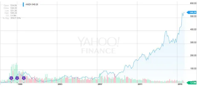
In Figure 4.1.1, the price per share of Amazon from September 4 to October 2 appears to experience a dramatic local rise. I had bought 100 shares from Amazon on September 26 at

(41)

30 about $524.25 per share. The share price raised about 1.58% from when I bought the stocks. The total gain of that week for that stock was $829. Amazon appears to be still on a steady, gradual rise so I still have confidence that the stock will continue.

Figure 4.1.1. Yahoo AMZN Sept 4 – Oct 2

However, the other stocks that I have invested in have not been performing to par. Apple and Bank of America have not experienced much change in the week. In fact, the net loss from both is under $200 combined. On the other hand, a company that I had thought was going to experience oscillation is steadily dropping.

I invested 5000 shares in OpGen on September 30 in high hopes that they would experience a jump in stock price because new smaller companies tend to have more significant changes in their stock prices. The charts that show their performance in the last month show that they had unpredictable behavior. I had hoped to catch OpGen in a falling state and try to sell when they rise again. I still believe that they will have more oscillation in the week. The total loss is $2,300 at this point for OpGen alone. Figure 4.1.2 shows OPGN’s prices.

(42)

31

Figure 4.1.2. Yahoo OPGN share price Sept 18 – Oct 2

Figure 4.1.3 shows Intel’s stock performance between September 18 and October 2.

Figure 4.1.3. Yahoo INTEL Sept 18 – Oct 2

Some of the companies that I decided not to invest in were in an uptrend in which I felt that if I had invested, then I would lose profit because it would be accompanied by a fall. I predict that Intel will experience a drop in stock price soon, most likely next week. If that is the

(43)

32 case, then I will invest because the general trend appears to be on a rise and if it falls, I predict it will rise again. Table 4.1.1 shows the transactions for week 1.

Table 4.1.1. Transactions for Week 1

Date Symbol Buy/Sell Price Shares Net

Cost/Proceeds Profit/Loss Total Cash Total Profit 9/23/2015 500000 9/25/2015 AMZN Buy $524.25 100 $52,432 $447,568 $0 9/30/2015 AAPL Buy $111.10 100 $11,117 $436,451 $0 9/30/2015 OPGN Buy $2.78 5000 $13,907 $422,544 $0 9/30/2015 BAC Buy $15.46 350 $5,418 $417,126 $0 9/30/2015 C Buy $48.53 200 $9,713 $407,413 $0 4.2 Week 2

Over the course of this week, there was not much change in the overall from these stocks. However, I was correct in thinking that OpGen would fluctuate during this week. In fact, in the first few days I had checked the stocks and found that it changed 20 percent at one point. However, I did not sell because I was hoping that it would rise even more. The 20 percent positive change actually evened out the initial investment for a zero net loss. I went out to pick up lunch and checked back again and found that it had dropped 8 percent in the total 2 minutes that I had gone out. In that time frame, about $800 of potential profit was lost. Smaller companies like OpGen show very unpredictable results. Table 4.2.1 shows the change after coming back to check on the company.

(44)

33

Table 4.2.1. Performance Oct 5 (Specific note on OPGN)

Another company that caught my interest was Tesla. In the past week, Tesla’s stock dropped very significantly. In Figure 4.2.2, the curve of the stock price and the simple moving average are displayed. The idea is that investing in Tesla now would be a good decision because based on the moving average, the stock has a good chance to converge back to the average in the next few weeks. I invested almost half my budget because I am confident that Tesla will be successful in the future.

(45)

34 For the other companies, investments were not made this week because of the fear that it would drop right after investing. In Figure 4.2.3, it should be apparent that the stocks are moving in a trend well above the moving average which indicates good performance, but induces a fear that the stocks will go back down. However, the best time to make the investment in Intel or Microsoft would have been the start of this week. The potential profit from each company would have been significant.

Figure 4.2.2. Yahoo INTEL & MSFT Oct 2 – Oct 10

The performance at the end of the week was decent. All companies seemed to have experienced a net profit, which is the desired result. Citigroup made a positive comeback after a loss from the previous week. However, OpGen continues to drop and may be raising a flag to prevent further losses. The overall net profit is merely a positive $334 but is more than satisfactory as no real losses ensued. The net gain actually went from negative to positive this week. Larger companies like Amazon show reliable and predictable trends whereas smaller companies require special attention to reap profit. In the end of this week, the time to sell is still unclear because each of the companies show promise, but the actually returns have yet to reach satisfactory values. Table 4.2.2 shows the progress for the week.

(46)

35

Table 4.2.2. Performance Oct 1

Table 4.2.1 shows the transactions for the second week 2. Only shares from Tesla were bought.

Table 4.2.3. Transactions Week 2

Date Symbol Buy/Sell Price Shares Net

Cost/Proceeds Profit/Loss Total Cash Total Profit 10/9/2015 TSLA Buy $220.69 1000 $220,697 $186,716 $0 4.3 Week 3

In this week, I spent time writing the code to retrieve data from a financial source (Yahoo Finance) using Matlab and its package Financial Toolbox. This toolbox allows the user to retrieve the high, low, open, and close prices of a specified stock. Using evaluation methods, the price for the day can be estimated by an average of these four components. After obtaining the graphs to reflect the data, I decided to analyze it using local extrema. I’ve set a window interval and a sensitivity value for the function to search for these critical points. From them, I can then

(47)

36 partition the graph in a way to reflect the trends that have occurred within the given period. Using these trends, I will select companies based on criteria that I will test such as moving averages, volume, and percent changes.

Samples of the GUI that retrieves data from Yahoo Finance are shown in Figure 4.3.1 and Figure 4.3.2 below.

(48)

37

Figure 4.3.2. Matlab AMZN Jul 1 – Oct 18

After reviewing what graphical indicators would be best to use for recognizing trends, I decided to base my first search on the last local trending period. To do this, I used the data fed from Yahoo Finance and manipulated it with the Financial Toolbox to generate a simple moving average data series. A function used to find local extrema was executed on this data set and the points were superimposed on the same graph. Lines were generated to connect these points to resemble a partitioning of the stock data. With this method, the program will have a way to know where uptrend and downtrends are located.

The last two points of the simple moving average were used to figure out whether the stock is currently rising or falling. However, although the moving average is a general indicator, the actual stock price may not at all reflect the same movement. For example, the actual price

(49)

38 may fluctuate in a way that would produce the image of a rising trend in its corresponding moving average. For this week, I will test a method that uses recent historical data.

A sample of the Matlab code has been provided below that iterates through an array of stock symbols and selects candidates that pass the conditional statements.

y1 = loc_extrema_mavg.pts(end,2); %gets last point

y2 = loc_extrema_mavg.pts(end-1,2); %gets second to last point

x1 = loc_extrema_mavg.pts(end,1); %gets last mavg datenum

x2 = loc_extrema_mavg.pts(end-1,1); %gets second to last mavg datenum

pct.rise = risePercentage(y2,y1); %gets percent rise

%checks for positive rise, trend interval, and within a bound

if (y1 - y2) > 0 && ...

(x1 - x2) > trendinterval && ...

pct.rise > pct.lowbound && ...

pct.rise < pct.highbound

%adds company to potential candidate list if

%criteria is met.

company = cellstr(company); stocklist = [stocklist;company]; end

The variables, y1, y2, x1, and x2 are obtained from the last two points of the moving average. The percent rise, pct.rise, is obtained using the last two values of the moving average relative to the point before the last. The percent rise is bounded by two limits to find stocks that are within a certain uptrend range. The trendinterval variable is to check how long the trend has been lasting.

I set the trend interval to 14 days, and the high and low bounds to 5.1% and 5.5% respectively. I wanted to limit the candidates down to a manageable range and also pick ones that are in a current rising trend. I picked these rise percentage limits because they are relatively moderate to factor out companies that have higher rises because they would be likely to fall as sharply resulting in loss in profit if I were to buy at that time.

After filling an array with 3280 stock symbols from the NYSE, the candidate program reduced the list to 26 potentials. I picked 5 of them that appeared to continue in the same trend based on how much fluctuation there is and its general motion.

(50)

39 Table 4.3.1 shows the transactions for week 3. I’ve decided to sell all the stocks from the previous week and try to trade based on the candidates that the program has picked and what I’ve learned from experience from the prior two weeks. I also partitioned them around $100,000 each see how they perform percentage-wise. Lastly, the prior two weeks netted a total positive gain approximately $12,000.00, which is good progress.

Table 4.3.1. Transactions for Week 3 Algorithm 1

Cost/Proceeds Profit/Loss Total Cash Total Profit 10/16/2015 C Sell $52.69 200 $10,531 $818 $211,040 $704 10/16/2015 TSLA Sell $227.01 1000 $227,003 $6,306 $438,043 $7,010 10/16/2015 AMZN Sell $570.73 100 $57,066 $4,634 $495,109 $11,644 10/16/2015 AAPL Sell $111.04 100 $11,097 -$20 $506,206 $11,624 10/16/2015 BAC Sell $16.12 350 $5,635 $217 $511,841 $11,841 10/16/2015 ACE Buy $108.95 1000 $108,957 $402,884 $11,841 10/16/2015 PKY Buy $16.97 5000 $84,857 $318,027 $11,841 10/16/2015 RTN Buy $111.30 900 $100,177 $217,850 $11,841 10/16/2015 CSC Buy $64.32 1700 $109,351 $108,499 $11,841 10/16/2015 TRC Buy $23.87 4000 $95,487 $13,012 $11,841 4.4 Week 4

In the fourth week, the results of previous week were obtained. All the stocks that had been purchased as candidates were sold and the profit/loss were recorded. Table 4.4.1 shows the transactions of week 4. The total profit rose to $25,472.99 which is more than doubled the previous week’s profit.

(51)

40

Table 4.4.1. Transactions for Week 4 Algorithm 1

Cost/Proceeds Profit/Loss Total Cash Total Profit 10/23/2015 ACE Sell $114.83 1000 $114,823 $5,866 $127,835 $17,707 10/23/2015 PKY Sell $17.09 5000 $85,443 $586 $213,278 $18,293 10/23/2015 RTN Sell $117.77 900 $105,986 $5,809 $319,264 $24,102 10/23/2015 CSC Sell $66.31 1700 $112,720 $3,369 $431,984 $27,471 10/23/2015 TRC Sell $23.35 4000 $93,393 -$2,094 $525,377 $25,377 10/23/2015 ASR Buy $158.01 600 $94,813 $430,564 $25,377 10/23/2015 JTA Buy $12.20 7500 $91,507 $339,057 $25,377 10/23/2015 SMP Buy $38.86 2500 $97,157 $241,900 $25,377 10/23/2015 STI Buy $41.75 2500 $104,382 $137,518 $25,377 10/23/2015 ESD Buy $14.37 7000 $100,597 $36,921 $25,377

In taking a closer inspection at Figure 4.4.1, the last two extrema of the simple moving average of the previous week, Oct 16, was clearly in an uptrend and the fluctuation amplitudes were not too unpredictable. We see that it continues in the rising trend, which was the predicted and desired direction.

(52)

41 Figure 4.4.2 below contains the stock, TRC, which was the only stock out of the five candidates that resulted in a loss of profit. Although the most recent trend was in an upward direction, the large fluctuations proved to be a danger. Before selling the stock, the price dropped below what it had been bought for. The initial idea of using the moving average, essentially sort of a “momentum”, is more reliable when the stock does not experience big fluctuation. In the case of TRC, the stock had shown a history of unstable price changes which is an indicator that it might be not a reliable candidate for this type of method. Another factor that will be incorporated in future methods will be the volume of trades. In all these graphs, heavy rises and falls correspond to the activity of trades in the market. “If the previous relationship between volume and price movements starts to deteriorate, it is usually a sign of weakness in the trend. For example, if the stock is in an uptrend but the up trading days are marked with lower volume, it is a sign that the trend is starting to lose its legs and may soon end.” [13]