Decentralized Policy Gradient Method for Mean-Field Linear Quadratic Regulator with Global Convergence

Decentralized Policy Gradient Method for Mean-Field Linear

Quadratic Regulator with Global Convergence

Lewis Liu [email protected]

Mila & DIRO, Universit´e de Montr´eal, Montreal, QC, Canada

Zhuoran Yang [email protected]

Princeton University, Princeton, NJ, USA

Yuchen Lu [email protected]

Mila & DIRO, Universit´e de Montr´eal, Montreal, QC, Canada

Zhaoran Wang [email protected]

Northwestern University, Evanston, IL, USA

Abstract

The scalability of multi-agent reinforcement learning methods to a large number of population is drawing more and more attention in both practice and theory. We consider the basic yet important model,i.e., linear quadratic regulator (LQR), in a mean-field approximation scheme against the curse of the action space dimensionality and the exponential growth of agent interactions. Several methods proposed in mean-field setting require a centralized controller, which is unrealistic in practice. In this paper, we present the first decentralized policy gradient method (MF-DPGM) for mean-field multi-agent reinforcement learning, where a large team of exchangeable agents communicate via a connected network. After a linear transformation of states and policies, we update the new local and mean-field policies by a decentralized gradient primal-dual algorithm respectively in a decoupling way, in order to achieve a global policy consensus. We also give a rigorous proof of the global convergence rate of MF-DPGM by studying the geometry of the problem and estimating one-step progress under decentralized scheme. In addition, extensive experiments are conducted to support our theoretical findings.

Keywords: Multi-Agent Reinforcement Learning, Decentralized Learning, Mean-Field Approxi-mation, Global Convergence

1. Introduction

Recent years have witnessed a promising resurgence of multi-agent reinforcement learning (MARL) in data-driven and large population environments. Motivating applications span over multi-robotics systems (Corke et al., 2005), autonomous driving (Lo, 2012; Shalev-Shwartz et al., 2016), and sensor networks (Rabbat and Nowak,2004;Cortes et al.,2004). MARL involves a set of agents learning to make decisions that minimize their accumulative cost by iterative interactions with a shared environment (Shoham et al.,2003,2007;Bu et al.,2008). As a result, a fundamental difficulty in MARL is that changes in the policy of one agent will affect that of the others, and vice versa (Matignon et al.,2012). What is worse, large modern multi-agent systems result in an exponential growth of the capacity of the joint action space with the number of agents. Hence the classical MARL methods (Bowling and Veloso,2002;Lipsa and Martins,2011;Lessard and Lall, 2015) via either equilibrium-solving or few controllers stagger in large-scale applications. Additionally, although a central controller receiving costs and determining actions reduces MARL to

a classical MDP which can be solved by existing single-agent RL approaches, the central controller is usually costly to install and the communication overhead degrades the scalability and robustness.

Motivation of mean-field settings. In this paper, we consider homogeneous large-scale MARL systems with symmetry, where each agent has the same reward function and state transition rule. To address the complicated correlations in multi-agent systems, Foerster et al.(2018) andPanait and Luke(2005) consider accounting for the extra information from conjecturing the policies of other agents, whileLee et al.(2018) andZhang et al.(2018a) study the decentralized actor-critic algorithm. On the other hand, the mean field approximation (Lasry and Lions,2007;Huang et al.,2006) serves as an effective alternative to modelling strategic interactions for large populations with symmetry. To characterize the mean-field effect in finite-agent systems, Arabneydi and Mahajan(2016) shows that any exchangeable system, where exchanging any two agents does not affect the dynamics or costs, is equivalent to one where the dynamics and costs are coupled across agents through the mean field (empirical mean state). More importantly, compared to other formulations, the mean-field setting greatly alleviates the curse of action space dimensionality by a symmetric global optimal policy and a cost function for all agents while decoupling complex correlations in large interactive systems.

However, neither decentralized algorithms nor accompanied guarantees are studied for the well-behaved mean-field setting. To fill this void, we study the decentralized exchangeable multi-agent systems in the collaborative setting where each agent seeks the optimal policy that minimizes the accumulative global cost over all the agents, via neighborhood communications by a connected network. We propose the first decentralized policy learning scheme with smaller exploration space, less communication, and more robustness. Moreover, we study the non-convex problem geometry by several almost continuity results, which are combined with one-step iterate progress to establish a sublinear global convergence rate for the simple yet fundamental setting LQR. Our contributions are concluded as follows: (1) We formulate the policy gradients for MARL under the mean-field setting. (2) We proposed the first decentralized algorithm (MF-DPGM) to effectively learn the optimal policy for mean-field MARL. (3) We present a novel global convergence guarantee for MF-DPGM under mild assumptions and simulation results to justiify the performance of our algorithm.

Related Work. There has been a line of work on solving normal MARL problems. Based on the seminal work for the framework of Markov games Littman (1994), follow-up works, such asLauer and Riedmiller(2000);Littman(2001);Hu and Wellman(2003), studied both collaborative and competitive relationships among agents. Recently, MARL with a large populationSandholm

(2010); Lo(2012) becomes increasingly popular, such as urban transportation Shalev-Shwartz et al.(2016);Lo(2012), social dilemmasLeibo et al.(2017);Hughes et al.(2018), multi-robotics systemsCorke et al.(2005), and power gridsCallaway and Hiskens(2010), wherein the curse of dimensionality for learning and controlMatignon et al.(2012) arises. Our work is in the line of collaborative settings, where a central controller can help solve MARL by existing single-agent algorithmsBradtke et al.(1994);Tu and Recht(2017);Malik et al.(2018). Nonetheless, due to high cost to set central controllers in large-scale applicationsKulkarni and Venayagamoorthy(2010), a series of decentralized methodsWai et al. (2018);Zhang et al. (2018a); Lee et al. (2018) are developed followingZhang et al.(2018b) to learn optimal policies with local rewards and actions.

Mean-field approximation of the system stems fromStanley(1971), which is generalized to multi-agent scenarios byHuang et al.(2003);Lasry and Lions(2006,2007);Huang et al.(2006). Our setting is also closely related to mean-filed control for exchangeable agentsMadjidian and Mirkin

(2014);Arabneydi and Mahajan(2016) but from a model-free reinforcement learning perspective. Although another independent simultanuous work (Carmona et al.,2019) investigate MARL for

a mean-field case, only the centralized algorithm with infinite players is considered and directly reduced to single-agent LQR when doing variable transformation.

Notations. In this section, we introduce some frequently used notations through the paper, while others will be defined as they are needed. We denote by[n]the set of integers{1,2, ..., n}, byN¯ all of the nonnegative integers. We useh·,·ito denote the inner-product for vectors, matrices, tensors, and block-wise cases according to the context. For a matrixX ∈_Rd×d_{and a vectorv ∈}

Rd, we

definekvk2

X :=v

>_{Xvas the squared norm ofvunder metric matrixX. Whenvis a matrix or tensor,} kvkrefers to the norm of its vectorization. Themode-n matrix productof tensorX ∈Rd1×···×dp

and a matrix X ∈ _Re×dn _{is a tensorX}

X(n) ∈ Rd1×···×dn−1×e×···×dp. Without specifying,XX

denotes mode-1 matrix product. We denote by1and0the all-one and all-zero vector (resp. tensor) respectively by the context, byσmin(X)the smallest eigenvalue ofX.

2. Problem Formulation

We study discrete-time linear-quadratic MARL under mean-field settings with exchangeable finiten agents. The states of the system at time-steptis given by{x(1)_t , x(2)_t ,· · ·, x_t(n)}, wherex(_ti)∈Rd

denotes the state vector of theithagent (i∈[n]). Then the system dynamics is described as follows, x_t(i₊₁) =Ax_t(i)+Bu(_ti)+ ¯Ax¯t+wt(i), ∀i∈[n], (2.1) whereu(_ti)∈_Rm _{denotes the control (the action), a Gaussian noisew}(i)

t ∼N(0, Id)independent of each agent and time-step is added to the succeeding state,x¯t= 1/nPni=1x

(i)

t denotes the mean-field state of the system at time-step t. For such dynamics, we have a collective cost function of the distributed system at time-stept,

ct= n

X

i=1

x_t(i)>Qx_t(i)+u(_ti)>Ru(_ti)+ ¯x>_tQ¯x¯t, (2.2) where we also define the cost for agentiasc(_ti)=x_t(i)>Qx(_ti)+u(_ti)>Ru(_ti)+ ¯x>_t Q¯x¯tat time-stept. Furthermore, it is shown that optimal control for theithagent can be written as a linear combination ofx(_ti) andx¯t,u(ti) = Kx

(i)

t +Lx¯t,where the same matrices{K, L} apply to all agents by the symmetry results in optimal control (Arabneydi and Mahajan,2016). By pluggingu(_ti)into (2.1), we can rewritex(_ti₊₁) asx_t(i₊₁) = (A+BK)x(_ti)+ ( ¯A+BL)¯xt+w(ti).LetΘ = (K;L)∈R2×m×d, beginning with initial states{x(₀i)}n

i=1, our goal is to find the controls{u (i)

t }ni=1(t≥0) minimizing

the long-term collective cost, C(Θ) =Ex0,w "_∞ X t=0 γtct # =Ex0,w ∞ X t=0 γt n X i=1 x(_ti)>Qx(_ti)+u_t(i)>Ru(_ti)+ ¯x>_t Q¯x¯t . (2.3) We denote byγ ∈(0,1)the discounted factor in the infinite horizon. The expectation is takenw.r.t.

all the initial statesx0 = x(1)0 >

, ..., x(₀n)>>

and all independent noise termsw={w(_ti)}_{i∈[n],t∈N}. Therefore, our goal is to solve the following infinite horizon mean-field LQR problem,

minimizeC(Θ)s.t. x_t(i₊₁) =Ax(_ti)+Bu(_ti)+ ¯Ax¯t+w(ti), x

(i)

0 ∼ Dfor eachi∈[n]. (2.4)

3. The Approach and Algorithm

To deal with the correlated states in the mean-field setting, we adopt the reparametrization trick in SectionAto obtain the dynamics below,

However, without a central controller theith agent possessesM(i) (i ∈[n]), which is defined as the policy iterate of theithagent in decentralized scenarios, as its local policy before convergence and is restricted to communicating policies with neighbor agents over a network, although each agent has access to the global mean state. Similar problems emerge when updatingN(i)’s, which is the mean-field policy of each agent before finding the optimum. Hence, we resort to performing a decentralized optimization scheme with global consensus. AsM andN are decoupled into two similar update processes, below we denote byΘe(i) eitherM(i) orN(i). We concatenate policy parameters together as a higher dimensional tensor,i.e.,Θe = [Θe(1);Θe(2);...;Θe(n)]∈Rn×m×dto give a compact formulation of the decentralized optimization problem:

min e Θ e C(Θe) := 1 n n X i=1 C(Θe(i)), s.t. Θe(i)=Θe(j) for (i, j)∈ E, (3.2) where the commumication network is considered as anunweightedandundirectedgraphG ={V,E}

with vertex setVand edge setE. Such a description gives a separable global objective functionCe(Θe) and linear constraints indicating the connectivity property of the communication network. In next section, we will introduce a more tractable formulation for algorithms by graph theory. Note that the summands in (3.2) are disjoint components ofΘe. Therefore, the gradient of the global objective should be expanded as:∇Ce(Θe) = 1/n ∇C Θe(1)

;...;∇C Θe(n)

.

Communication Structure and Algerabic Representations.Below we capture the structure ofG

with|V|=nand|E|=eby some tools from spectral graph theory. Define the edge-associated (Ωθ) and agent-associated (Γθ) parametersΩθ = diag(σ1θ,· · · , σeθ) 0,Γθ = diag(γ1θ,· · ·, γnθ) 0, whereθcan be replaced byMorN to represent two sets of configurations since the policy parameters are decoupled into two optimization processes. Hereafter if we use symbols without specifyingM or N, the statement will hold for bothMandN, respectively. We will see how they serve as step-size for MF-DPGM in Section3.1. We also useσij, where(i, j) ∈ E is thekth edge also denoted as i∼j, as an alternative toσk. The quantity assigned to agentiis used forM(i)orN(i), or both by the context. Denoting the graph Laplacian matrix and its normalized versionChung and Graham

(1997) as Land Lerespectively, we defineLa := |L| ∈e Re×n by taking element-wise absolute value onLe. By definitions we can find the following relation: D = 1/2(Le>Le+L>_aL_a),where D= diag(d1, ..., dn)withdias the degree of vertex (agent)i. For further proof, by calculation we defineΩ := diage _n P j:j∼iσ2ij o j∈G = 1/2(Le>Ω2Le+LaΩ2La),H := La>Ω2L+ Γ2., and η_i2 = 2P

j:j∼iσij2 +γi2. With these parameters, we can rewrite (3.2) in a more tractable form for numerical algorithms:min

e

ΘCe(Θe) := 1/n

Pn

i=1C(Θe(i)), s.t.LeΘe₍₁₎=0. The idea of MF-DPGM relies on this formulation from a primal-dual view.

3.1 The MF-DPGM Algorithm

The overall MF-DPGM can be split into following steps.

Initialization: Similar to Prox-MMWright(1990), our method first initialize the policy parameter e

Θ(₋₁i) M₋₁(i);N₋₁(i)of agentiwith zeros at iteration -1, and then endow policies at step 0 withΘe

(i) −1’s.

Such a setup benefits further updates by controlling the constants of theoretical bounds in Section4.

Policy running and evaluation: At the beginning of thekth iteration, we samplenp trajectories of each agentiaccording to its own current policyΘe

(i)

k , to estimate the action-value function by

1/npPnp=1p Qbπ_i,p(x

(i)

t , u

(i)

t ) for policy evaluation in model-free settings1. Furthermore, to retain

1. Also, we can share part of noise with termu(ti)in2.1to make stochastic policies. To highlight our main idea, we focus

Algorithm 1:Mean-Field Decentralized Policy Gradient Method (MF-DPGM)

Data:Agent dynamicsn, A, B,A¯; Cost parametersQ, R,Q¯; Initial state distributionD.

Input:NetworkG;Ω,Γ; Length of horizonT; Number of sample pathsnp; Estimation error. Output: Estimation of optimal control policiesΘb.

Initialization:Θe−1=0;Θe (i) 0 =∇C(i)(0)η −2 i /n,∀i∈[n]; Iterationk←1. whileε(k)> do forpath p = 1 tonpdo fort = 1 to Tdo u_t(i)=M_k(i)y_t(i)+N_k(i)y¯t; x(_ti₊₁) ←Ax(ti)+Bu (i) t + ¯A¯xt+w (i)

t , for alli∈[n]in paralell;

b Qπ i,p(x (i) t , u (i) t )← PT s=tγ s−t_c(i) s ; end end Compute∇C(b Θe (i) k )←1/np Pnp p=1 PT t=1Qbπ_i,p(x (i) t , u (i) t )· ∇logπΘb(i)(u (i) t |x (i) t ), for alli∈[n] Communication and update:For alli∈[n],

e Θ(_ki₊₁) ←Θe (i) k − 1 (ηθ i)2 1 n ∇Cb Θe (i) k − ∇Cb Θe (i) k−1 −2 X j:j∼i (σ_ijθ)2Θe (j) k + (γ θ i) 2 e Θ(_ki₋₁) −Θe (i) k + X j:j∼i (σθ_ij)2Θe (j) k−1+Θe (i) k−1 (3.3) b Θ←Θek,k←k+ 1 end

accuracy for large populations, we adopt gradient estimator in REINFORCESutton et al.(2000) for the cost function instead of the biased zeroth order methodFazel et al.(2018). In practice, the deterministic policyu(_ti)can be realized by a Gaussian policyπ_Θ(i) with a nearly zero variance. Communication and update: After running policies at the kth iteration, each agent i collects policies from neighbors and its own gradient estimators of the cost function at thekthand(k−1)th

iterations, and combines them linearly byΩθandΓθ as a decentralized version of policy gradient methodBaxter and Bartlett(2001) to update the local policyΘe

(i)

k . As a result, we can view tunable parameters Ωθ and Γθ as step-sizes in MF-DPGM. See (3.3) for a detailed update. A practical choice (Gemulla et al.,2011;Shi et al.,2015) isΩ2_θ :=α2I as a multiple of identity,

A full description of MF-DPGM is shown in Algorithm1. Due to decentralized nature, our convergence measure,ε(t) = mins∈[t]

1/n Pn i=1C(Θe (i) s )−Ce(Θe∗) +kΩL{e Θek}(1)k 2_fort∈N¯_,

not only takes cost error into account, but also consider consensus error to guarantee an identical optimal policy in Section2. See AppendixBfor a connection with the primal-dual paradigm. 4. Theoretical Results and Analysis

As many other dencentralized algorithms, our convergence results also rely on some smoothness property (Lipschitzness of the gradient) of the objective. However, we notice that the optimization landscape for each agent is not strictly smooth due to unstability ofA+BM (resp.A+ ¯A+BN). At the boundary between stable and unstable policies, the cost function rapidly becomes infinity, which violates the traditional smoothness conditions. To address this issue, we regulate the parametersΩ

andΓfor a small step-size to set the next iterateΘe

(i)

t+1sufficiently close to the current one, so that: Σ e Θi t+1 ≈Σ e Θi t +OkΘei_t+1−Θei_tk

the continuity property of the cost functions, state trajactories, and gradients of cost corresponding to policyM andNwithin an adaptive area for each agent. Accordingly, we have the following

condition on edge and agent associated parameters,i.e. ΩandΓto guarantee the development of our decentralized update.

Condition 4.1. The parameters of MF-DPGM are chosen to satisfy for anyk≥1andi∈[n],

Ωθ+ Γ2θ /2(2c+ 1)Φθ/n+ 4κΦθΓ−2_θ Φθ/n2, c= max{1,6κ}, Γ2θΦθΓ−2_θ Φθ/n2, (4.1) γ_i2F_θ(θ(_ki))−nγ 2 i +βi n Fθ(θ (i) k−1)≥ X j:j∼i σ_ij2 kθ(_ki)k+kθ(_ki₋₁) k+F_θ(θ(_kj₋₁) )−2F_θ(θ_k(i)), (4.2) whereκ = 1/λmin ΩF H−1FTΩ

, (4.2) admits two sets of conditions when replacingθ byM orN exclusively, along withF_M(X) = min{ξσmin(Q)/[4(kA+BXk+ 1)· kBk ·C(X)],kXk}

andFN(X) = min

_¯

ξσmin(Q+ ¯Q)/[4(kA+BXk+ 1)· kBk ·C(X)],kXk , SimilarlyΦM =

diag(β₁M, ..., β_nM)⊗Imd∈Rnmd×nmdandΦN = diag(β1N, ..., βnN)⊗Imdare almost-smoothness constants specified in LemmaF.2.

We can see from proof thatκencodes the network structure andchelps construct the potential function indicating one-step progress of MF-DPGM. By properly choosingΩθandΓθ, we can meet the condition, so that potential function (E.1) decreases and boundary condition (F.9) of two adjacent iterates is met by dynamically adjusting as the adaptive area in (F.9), which is illustrated inF.3. Below we layout the global convergence result.

Theorem 4.2. Given Condition4.1, then for time-stept≥1, MF-DPGM gives

min s∈[t] 1 n n X i=1 C(Θe(_si))−Ce(Θe∗) +kΩL{e Θe_s}₍₁₎k2≤ 8α_gCC0/t | {z }

cost error bound

+ 20C0/t | {z }

consensus error bound

, (4.3)

where αg = max{αMg , αNg } with αMg = kΣM∗k/[σ_min(Σ(i)

0 )2σmin(R)] and αNg =

kΣN∗k/[σmin(Σ0)2σmin(R)]is a problem related constant for gradient domination also

appear-ing in LemmaF.3,Θe∗indicates the optimal policy parameters, and

C0 :=Ce(Θe₀)−Ce(Θe∗) + 2∇C(0)>Φ−1∇C(0)/n, C:= 4 X (i,j):i∼j σ2_ij+ n X i=1 γ2_i. (4.4)

Proof. See AppendixF.5for a detailed proof.

The main upshot is to characterize in detail the first global sublinear convergence rate for the overall error including the cost and consensus components. More precisely, MF-DPGM not only drives the average cost of agents to the optimal cost over time, but also guarantees heading for the same optimal policy. An alternative way to display the rates is distributedly showing for each agent with slightly different constants whereC0 is decomposed for each. Moreover, the optimization ofΘe can be split into development of local and mean-field policy respectively, which is frequently observed in theoretical illustration and proof, while the difference sits between the only one mean-field state associated withN(i)’s and corresponding multiple states forM(i)’s.

5. Conclusion

In this paper, focusing on a simple yet fundamental model LQR under the mean-field setting, we propose the first decentralized policy gradient method where each agent update the local policy by combining policies from neighborhood with its own policy. which is applicable to complex mean-field models. In addition, we quantify the non-convex problem geometry by several almost continuity results, which is combined with one-step progresses for our algorithm to establish a sublinear global convergence rate for LQR. Additional experiments justify our theoretical results and show a promising performance.

References

Jalal Arabneydi and Aditya Mahajan. Linear quadratic mean field teams: Optimal and approximately optimal decentralized solutions. arXiv preprint arXiv:1609.00056, 2016.

Jonathan Baxter and Peter L Bartlett. Infinite-horizon policy-gradient estimation.Journal of Artificial

Intelligence Research, 15:319–350, 2001.

Sergio Bittanti, Alan J Laub, and Jan C Willems.The Riccati Equation. Springer Science & Business Media, 2012.

Michael Bowling and Manuela Veloso. Multiagent learning using a variable learning rate. Artificial

Intelligence, 136(2):215–250, 2002.

Steven J Bradtke, B Erik Ydstie, and Andrew G Barto. Adaptive linear quadratic control using policy iteration. InProceedings of 1994 American Control Conference-ACC’94, volume 3, pages 3475–3479. IEEE, 1994.

Lucian Bu, Robert Babu, Bart De Schutter, et al. A comprehensive survey of multiagent reinforcement learning.IEEE Transactions on Systems, Man, and Cybernetics, Part C (Applications and Reviews), 38(2):156–172, 2008.

Duncan S Callaway and Ian A Hiskens. Achieving controllability of electric loads. Proceedings of

the IEEE, 99(1):184–199, 2010.

Ren´e Carmona, Mathieu Lauri`ere, and Zongjun Tan. Linear-quadratic mean-field reinforcement learning: convergence of policy gradient methods. arXiv preprint arXiv:1910.04295, 2019. Fan RK Chung and Fan Chung Graham.Spectral graph theory. Number 92. American Mathematical

Soc., 1997.

Peter Corke, Ron Peterson, and Daniela Rus. Networked robots: Flying robot navigation using a sensor net. InRobotics research. The eleventh international symposium, pages 234–243. Springer, 2005.

Jorge Cortes, Sonia Martinez, Timur Karatas, and Francesco Bullo. Coverage control for mobile sensing networks. IEEE Transactions on robotics and Automation, 20(2):243–255, 2004. Maryam Fazel, Rong Ge, Sham M Kakade, and Mehran Mesbahi. Global convergence of policy

gradient methods for the linear quadratic regulator. arXiv preprint arXiv:1801.05039, 2018. Jakob Foerster, Richard Y Chen, Maruan Al-Shedivat, Shimon Whiteson, Pieter Abbeel, and Igor

Mordatch. Learning with opponent-learning awareness. In Proceedings of the 17th

Interna-tional Conference on Autonomous Agents and MultiAgent Systems, pages 122–130. International

Foundation for Autonomous Agents and Multiagent Systems, 2018.

Rainer Gemulla, Erik Nijkamp, Peter J Haas, and Yannis Sismanis. Large-scale matrix factorization with distributed stochastic gradient descent. InProceedings of the 17th ACM SIGKDD international

Mingyi Hong, Zhi-Quan Luo, and Meisam Razaviyayn. Convergence analysis of alternating direction method of multipliers for a family of nonconvex problems. SIAM Journal on Optimization, 26(1): 337–364, 2016.

Junling Hu and Michael P Wellman. Nash q-learning for general-sum stochastic games. Journal of

machine learning research, 4(Nov):1039–1069, 2003.

Minyi Huang, Peter E Caines, and Roland P Malham´e. Individual and mass behaviour in large population stochastic wireless power control problems: centralized and nash equilibrium solutions.

In42nd IEEE International Conference on Decision and Control (IEEE Cat. No. 03CH37475),

volume 1, pages 98–103. IEEE, 2003.

Minyi Huang, Roland P Malham´e, Peter E Caines, et al. Large population stochastic dynamic games: closed-loop mckean-vlasov systems and the nash certainty equivalence principle.Communications

in Information & Systems, 6(3):221–252, 2006.

Edward Hughes, Joel Z Leibo, Matthew Phillips, Karl Tuyls, Edgar Due˜nez-Guzman, Antonio Garc´ıa Casta˜neda, Iain Dunning, Tina Zhu, Kevin McKee, Raphael Koster, et al. Inequity aversion improves cooperation in intertemporal social dilemmas. In Advances in Neural Information

Processing Systems, pages 3326–3336, 2018.

Duˇsan Jakoveti´c, Jos´e MF Moura, and Joao Xavier. Linear convergence rate of a class of distributed augmented lagrangian algorithms. IEEE Transactions on Automatic Control, 60(4):922–936, 2014. Raghavendra V Kulkarni and Ganesh Kumar Venayagamoorthy. Particle swarm optimization in

wireless-sensor networks: A brief survey.IEEE Transactions on Systems, Man, and Cybernetics,

Part C (Applications and Reviews), 41(2):262–267, 2010.

Jean-Michel Lasry and Pierre-Louis Lions. Games ˙a middle field. ii - finite horizon and control ˆo the optimal. Math ´e Math Accounts, 343(10):679–684, 2006.

Jean-Michel Lasry and Pierre-Louis Lions. Mean field games. Japanese journal of mathematics, 2 (1):229–260, 2007.

Martin Lauer and Martin Riedmiller. An algorithm for distributed reinforcement learning in coop-erative multi-agent systems. InIn Proceedings of the Seventeenth International Conference on

Machine Learning. Citeseer, 2000.

Donghwan Lee, Hyungjin Yoon, and Naira Hovakimyan. Primal-dual algorithm for distributed reinforcement learning: distributed gtd. In2018 IEEE Conference on Decision and Control (CDC), pages 1967–1972. IEEE, 2018.

Joel Z Leibo, Vinicius Zambaldi, Marc Lanctot, Janusz Marecki, and Thore Graepel. Multi-agent reinforcement learning in sequential social dilemmas. InProceedings of the 16th Conference

on Autonomous Agents and MultiAgent Systems, pages 464–473. International Foundation for

Autonomous Agents and Multiagent Systems, 2017.

Laurent Lessard and Sanjay Lall. Optimal control of two-player systems with output feedback.IEEE

Gabriel M Lipsa and Nuno C Martins. Remote state estimation with communication costs for first-order lti systems. IEEE Transactions on Automatic Control, 56(9):2013–2025, 2011. Michael L Littman. Markov games as a framework for multi-agent reinforcement learning. In

Machine learning proceedings 1994, pages 157–163. Elsevier, 1994.

Michael L Littman. Value-function reinforcement learning in markov games. Cognitive Systems

Research, 2(1):55–66, 2001.

Steven KC Lo. A collaborative multi-agent message transmission mechanism in intelligent trans-portation system–a smart freeway example. Information Sciences, 184(1):246–265, 2012. Daria Madjidian and Leonid Mirkin. Distributed control with low-rank coordination. IEEE

Transac-tions on Control of Network Systems, 1(1):53–63, 2014.

Dhruv Malik, Ashwin Pananjady, Kush Bhatia, Koulik Khamaru, Peter L Bartlett, and Martin J Wainwright. Derivative-free methods for policy optimization: Guarantees for linear quadratic systems. arXiv preprint arXiv:1812.08305, 2018.

Laetitia Matignon, Guillaume J Laurent, and Nadine Le Fort-Piat. Independent reinforcement learners in cooperative markov games: a survey regarding coordination problems. The Knowledge

Engineering Review, 27(1):1–31, 2012.

Liviu Panait and Sean Luke. Cooperative multi-agent learning: The state of the art. Autonomous

agents and multi-agent systems, 11(3):387–434, 2005.

James A Preiss, S´ebastien MR Arnold, Chen-Yu Wei, and Marius Kloft. Analyzing the variance of policy gradient estimators for the linear-quadratic regulator. arXiv preprint arXiv:1910.01249, 2019.

Michael Rabbat and Robert Nowak. Distributed optimization in sensor networks. InProceedings

of the 3rd international symposium on Information processing in sensor networks, pages 20–27.

ACM, 2004.

Dominic Richards and Patrick Rebeschini. Optimal statistical rates for decentralised non-parametric regression with linear speed-up. InAdvances in Neural Information Processing Systems, pages 1214–1225, 2019.

R Tyrrell Rockafellar. Augmented lagrangians and applications of the proximal point algorithm in convex programming. Mathematics of operations research, 1(2):97–116, 1976.

William H Sandholm. Population games and evolutionary dynamics. MIT press, 2010.

Shai Shalev-Shwartz, Shaked Shammah, and Amnon Shashua. Safe, multi-agent, reinforcement learning for autonomous driving. arXiv preprint arXiv:1610.03295, 2016.

Wei Shi, Qing Ling, Gang Wu, and Wotao Yin. Extra: An exact first-order algorithm for decentralized consensus optimization. SIAM Journal on Optimization, 25(2):944–966, 2015.

Yoav Shoham, Rob Powers, and Trond Grenager. Multi-agent reinforcement learning: a critical survey. Web manuscript, 2003.

Yoav Shoham, Rob Powers, and Trond Grenager. If multi-agent learning is the answer, what is the question? Artificial Intelligence, 171(7):365–377, 2007.

H Eugene Stanley. Phase transitions and critical phenomena. Clarendon Press, Oxford, 1971. Haoran Sun and Mingyi Hong. Distributed non-convex first-order optimization and information

processing: Lower complexity bounds and rate optimal algorithms. In 2018 52nd Asilomar

Conference on Signals, Systems, and Computers, pages 38–42. IEEE, 2018.

Richard S Sutton, David A McAllester, Satinder P Singh, and Yishay Mansour. Policy gradient meth-ods for reinforcement learning with function approximation. InAdvances in neural information

processing systems, pages 1057–1063, 2000.

Stephen Tu and Benjamin Recht. Least-squares temporal difference learning for the linear quadratic regulator. arXiv preprint arXiv:1712.08642, 2017.

Hirofumi Uzawa. Iterative methods for concave programming. Studies in linear and nonlinear

programming, 6:154–165, 1958.

Hoi-To Wai, Zhuoran Yang, Princeton Zhaoran Wang, and Mingyi Hong. Multi-agent reinforcement learning via double averaging primal-dual optimization. In Advances in Neural Information

Processing Systems, pages 9649–9660, 2018.

Stephen J Wright. Implementing proximal point methods for linear programming. Journal of

optimization Theory and Applications, 65(3):531–554, 1990.

Bin Yu. Rates of convergence for empirical processes of stationary mixing sequences. The Annals of

Probability, pages 94–116, 1994.

Kaiqing Zhang, Zhuoran Yang, and Tamer Basar. Networked multi-agent reinforcement learning in continuous spaces. In2018 IEEE Conference on Decision and Control (CDC), pages 2771–2776. IEEE, 2018a.

Kaiqing Zhang, Zhuoran Yang, Han Liu, Tong Zhang, and Tamer Bas¸ar. Fully decentralized multi-agent reinforcement learning with networked agents. arXiv preprint arXiv:1802.08757, 2018b.

Appendix A. Policy Gradient with Reparametrized States

In this section, we provide the details for Reparametrizing states in mean-field dynamics in Section3, as direct policy gradients over the matrix parametersK and Llead to gradients ofK (resp. L) containing the other parameterL(resp. K) due to the correlation mean-field termx¯tacross different agents, which is hard to apply analysis of standard policy gradients.

We characterize the optimal cost from a state going forward (see Eq. (A.6)) with (algebraic) Riccati equations (Bittanti et al.,2012) governed by policy parameters (i.e.,K, L). Note that in the formulation of the previous section, it is hard to directly obtain the optimal controlu(_ti)’s depending on bothx(_ti)’s andx¯t’s correlated in a single dynamics. Hence we adopt the following reparameterization method to derive decoupled Riccati equations.

u(_ti)=Kx_t(i)+Lx¯t=M(xt(i)−x¯t) +Nx¯t,M y(ti)+Ny¯t. (A.1) where we call M = K the optimallocal policyandN =K +Lthe optimalmean-field policy. Below we show how to derive policy gradient to update these policy parameters separately. We rewrite the dynamic equations below:

y(_t+1i) = (A+BM)y_t(i)+w_t(i)−w¯t, y¯t+1= [A+ ¯A+BN]¯yt+ ¯wt, (A.2) wherew¯t= 1/nPni=1w (i) t . Then we have C(Θ) =Ey0∼D,w ∞ X t=0 γt n X i=1 y(_ti)>(Q+M>RM)y_t(i)+ny¯_t>(Q+ ¯Q+N>RN)¯yt (A.3) = n X i=1 Tr[(Q+M>RM)Σ(_Mi)] +nTr[(Qe+N>RN)Σ_N], where Σ(_Mi) = Ey0∼D,w[ P∞ t=0γty (i) t y (i) t > ], ΣN = Ey¯0∼D¯,w P∞ t=0γty¯ty¯ > t , Qe = Q+ ¯Q, D

denotes thei.i.d. initial state distribution of y₀(i), andD¯ indicates the distribution of mean-field

¯

y0. We will omit the explicit distributions for expectations without ambiguity. With an abuse of

notations, letC(M(i)) = Tr[(Q+M>RM)Σ(_Mi)], C(N) = nTr[(Qe+N>RN)Σ_N], C(M) =

min_i∈[n]Tr[(Q+M>RM)Σ (i)

M]. From Bellman equation for cost functions, it follows that CΘ(y0) = n X i=1 y₀(i)>(Q+M>RM)y₀(i)+ny¯0P¯Ny¯0 +γEw0CΘ(diag(A+BM)y0+w0−w¯0), (A.4)

whereCΘ(y)is the value function with initial statey,diag(X)denotes thend×ndblock-diagonal

matrix with matrixX ∈_Rd_{being the block elements. We assume that the value function takes a} quadratic formCΘ(y0) =Pn i=1y (i) 0 > PMy0(i)+ny¯0>P¯Ny¯0+αΘ,wherePM,P¯N ∈Rd×dand we

ignore the cross terms as E[y0>P¯Ny¯0] = 0. LetAy = A+BM,A¯y = A+ ¯A+BN, then by Bellman equation (_n A.4), we have

X i=1 y(₀i)>PMy(₀i)+ny¯0>P¯Ny¯0+αΘ= n X i=1 y₀(i)>[γA>_yPMAy+Q+M>RM]y(₀i) +ny¯>₀[Q+ ¯Q+ ¯N RN+γA¯>_yP¯NA¯y]¯y0+γ n+ 1 n TrPM +γTrP¯N +γαΘ, (A.5)

which implies PM =Q+M>RM+γA>yPMAy, αΘ= γ 1−γ n+ 1 n TrPM + ¯PN , (A.6) ¯ PN =Q+ ¯Q+N>RN+γA¯>yP¯NA¯y.

HenceMandN are decoupled for Riccati equations after transformation.The gradient with respect toM in (A.4) gives ∇_MCΘ(y0) = (2RM + 2γB>PMAy) n X i=1 y(₀i)y₀(i)>+γE∇MCΘ(y1). (A.7)

By applying recursionyt+1= (A+BM)yt+wt(i)−w¯t(t≥0) to (A.7) iteratively, we can finally obtain ∇MCΘ(y0) = 2 RM +γB>PMAy _Xn i=1 Ey0,w ∞ X t=0 γty(_ti)y_t(i)> = 2RM +γB>PMAy _Xn i=1 Σ(_Mi) ,2ΞM n X i=1 Σ(_Mi). (A.8) Similarly, we have ∇_NCΘ(y0) = 2 RN+γB>P¯NA¯y ΣN ,2ΞNΣN. (A.9) TheΣN in∇NCΘ(y0)is a shared expectation term for all the agents resulted from mean-field states.

Appendix B. A primal-dual view on MF-DPGM

To see this, we demonstrate the neat connection between our algorithm and primal-dual paradigm commonly used for solving constrained programming. Let us introduce the augmented Lagrangian function (A) in tensor variables:

Ak :=A(Θe_k,Λ_k) =Ce(Θe_k) +hΛ_k,L{e Θe_k}₍₁₎i+ 1 2 ΩhL{e Θe_k}₍₁₎ i (1) 2 , (B.1) where Λk ∈ Re×m×d is the dual variable at iteration k, which is updated as Λk+1 = Λk +

ΩhL{e Θe_k}₍₁₎ i

(1)(*). By plugging this into (3.3) and using definition ofHwe have

∇Ce(Θe_k) +H(Θe_k+1−Θe_k)₍₁₎+L{e Θe_k}₍₁₎+Le>Ω2L{e Θe_k+1}₍₁₎ =0. (B.2) Viewing (B.2) as the optimal (first-order) condition of some function, we observe that update (3.3) is equivalent to e Θk+1= arg min e Θ D ∇C(Θe_k) +Le>Λ_k(1),Θe −Θe_k E +1 2kΩLeΘe(1)k 2₊1 2 ΩL_aΘe −Θe_k (1) 2 +1 2 ΓΘe −Θe_k (1) 2 (B.3) together with (*), where the third term of (B.3) encodes the network structure that we utilized for neighborhood average. Terms like kΩLeΘe₍₁₎k2 show how close policies of agents to each other are with policy Θe by definitions in § ??. Such a primal-dual interpretation is closely re-lated to some classical comstrained optimization methods, such as the Uzawa method Uzawa

0 100 200 300 400 500 600 Steps 0.020 0.025 0.030 0.035 0.040 0.045 0.050 Op tim ali ty Ga p complete random grid circle

(a) 3-dimensional dynamics

0 50 100 150 200 Steps 0.040 0.045 0.050 0.055 0.060 Op tim ali ty Ga p complete random grid circle (b) 4-dimensional dynamics 0 25 50 75 100 125 150 175 Steps 0.070 0.075 0.080 0.085 0.090 0.095 0.100 0.105 Op tim ali ty Ga p complete random grid circle (c) 5-dimensional dynamics

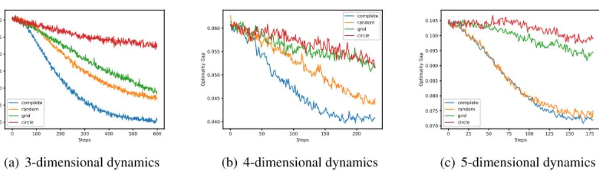
Figure 1: Simulation results (convergence curves) on complete (blue), random (orange), grid (green) and circle (red) networks, as well as different dynamicsd= 3,4,5.

(1958) and the prox-MM Rockafellar(1976);Wright (1990). Following distributed constrained optimization approaches Jakoveti´c et al. (2014); Hong et al. (2016), we set the error ε(t) = mins∈[t] 1/n Pn i=1C(Θe (i) s )−Ce(Θe∗) +kΩL{e Θek}(1)k

2_{fort∈N¯ to monitor consensus.}

Appendix C. Simulation and Result Analysis

We conduct simulation experiments shown in Figure1(a)-1(c), where we synthesize three different multi-agent systems by specifying dynamics parametersA, B,A¯and cost parametersQ, R,Q. under¯ the LQR setting each withd = 3,4,5, n = 25, and action spacem = d; See AppendixD for more setup details. We can see from the numerical results that when fixing the dynamics, different topologies of communication networks lead to diverse performances. The convergence rate ranges from the best to the worst over complete, random, grid, and circle graphs respectively. This reveals the influence of communication structure in control for large coupled systems, where a decentralized algorithm achieves an performance improvement as more possible communication links among agents are established. Moreover, it is shown that the dynamics settings also have an impact on the number of iterations to achieve convergence and stability. More precisely, the system with lower dimension enjoys a faster and stable convergence, which corresponds to the constantαgof the overall bound in Theorem4.2.

Furthermore, We plot the convergence curves in Figure2(a)for different numbers of agents to show the effectiveness of our method at different scales, where we also justify that the mean-field approximation works better as the size of the population grows by the increasing performance with the larger population, as the effect of mean-field phenomenon is more significant in larger systems. In addition, although it is unfair to compare against the centralized setting, where the controller has access to the costs of all agents and updates their policies simultaneously and identically, we plot the comparison in Figure2(b)for identification withn= 25. We reproduce a baseline of decentralized policy gradient with gossip matrices (Richards and Rebeschini,2019), which aggregates the updated policies from the neighborhood (aggreg. neighbor). Note that our algorithm compares favorably against this baseline and is competitive with the centralized one, which gives a better performance achievable.

0 50 100 150 200 250 300 Steps 5.0 5.5 6.0 6.5 7.0 7.5 8.0 8.5 Op tim ali ty Ga p nb_agents=30 nb_agents=40 nb_agents=50 nb_agents=60

(a) Convergence curves on different popula-tionsnover a circle graph.

(b) Comparison with baselines on a cir-cle graph.

Figure 2: Simulation results with different size of populations and comparison with baselines. Appendix D. Experiment Setup and Additional Details

In this section, We provide additional configuration details and analysis of the experimental results in SectionC.

Experiment setup. In the experiement we intend to demonstrate the convergence performance of our algorithm under different graph structures and different dynamics. We consider policy learning with global consensus as follows:

min e Θ e C(Θe) := 1 n n X i=1 C(Θe(i)), s.t. Θe(i)=Θe(j) for (i, j)∈ E, (D.1) where for alli,

x_t(₊₁i) =Ax(_ti)+Bu_t(i)+ ¯Ax¯t+w(ti), (D.2) c_t(i) =x_t(i)>Qx(_ti)+u_t(i)>Ru(_ti)+ ¯x>_t Q¯x¯t. (D.3) The state transition matrixA, B,A¯is generated by first sampling a random uniform matrix from 0 to 1 and then tossing a biased coin with probability 0.7 for setting each element zero to keep sparsity for computational efficiency. Also, such transition matrices may lead to smoother loss surfaces. For the reward function we adopt diagonal matrices with each element on the diagonal from 0 to 1 and sparse perturbation for off-diagonal entries. We test on four different graphs as the communication networkG: 1) complete graph 2) grid graph 3) circle graph and 4) random graph. The random graph is essentially an Erdos-R´enyi graph generated with connectivity of 0.25. Alternatively, for each pair (i, j) with i ∈ [n], j ∈ [n], we toss a coin to decide whether there will be an edge between agentiand agentj. As we toss coins two times for both (i, j) and (j, i), an equivalent random graph is obtained with 0.75 probability for each edge to vanish. We setΩ2 = Γ2 =I as identity matrices to better understand the popular average of neighborhood scheme. The results of convergence curves are presented in Figure1(a)-1(c), where y-axis denotes the error measure ε(t) = min_s∈[t] 1/n Pn i=1C(Θe (i) s )−Ce(Θe∗) +kΩL{e Θek}(1)k 2_fort∈N¯_.

For the impact of the topology of the communication graphs on the convergence rate, when choosingΩandΓaccording to Section4, we can easily verify that the condition (4.1) holds, so that constantCof the bound in Theorem4.2can be reparameterized as follows,

C ≤ 320 max{σmax(Z),1} min{σ_min(LG),1} X i∼j p βiβj p didjn +β¯ 4 ! , (D.4)

whereβ¯= 1/nPn

i=1βi;see more details inSun and Hong(2018). Hence the global rate is connected to the algebraic summary,i.e., spectral gap, that captures the connectivity of the communication network, which quantifies how the connectivity of four different graphs impacts convergence perfor-mance of MF-DPGM.

For the impact of the dimension of dynamics on the convergence, high dimensions have a higher chance to introduce high variance inΣ(₀i)depending on the initial random states, and different cost dynamics also account a change in αg. In addition, we observe that performance gap between complete graph and other two deterministic graphs increases in higher dimension configuration, which implies an interplay between communication structure (C) and system dynamics (αg) in the convergence rate.

Appendix E. Proof Sketch

We sketch the proof of results in Section 4. Define Σ(₀i) := Ey(0i)y (i) 0 > , Σ0 := Ey¯0y¯>0, ξi := σmin(Σ(0i)),ξ¯=σmin(E_y(i) 0 ∼D ¯

y0y¯0>), whereσmin(X)denotes the smallest singular value ofX. We

denote byσ_min(X)the second smallest eigenvalue ofX.

Geometry of cost functions. As mentioned in Section4, Theorem4.2requires moderate smoothness of the landscape of cost functions. Based on the almost Lipschitzness of positive definite matrix Pθparameterizing the optimal cost from a state going forward, and almost Lipschitzness of theΣθ which plays an key role in cost function. LemmaF.2for each cost function with an almost Lipschitz gradient and Lemma F.3 for each cost function almost dominated by the gradient are crucial in bounding the one-step differences in LemmaF.6andF.7.

Progress of decentralized iterations.To estimate one-step progress of Algorithm1, we con-struct the auxiliary potential functionU to show certain monotonicity along the solution path in both primal (Θe) and dual (Λ) variables:

Uk+1 =Uc e Θk+1,Θe_k,Λ_k+1 :=A_k+1+2κ n2 Γ −1_Φ e Θk+1−Θe_k 2 (E.1) +c 2 ΩL{e Θek+1}(1) 2 + Θek+1−Θek 2 H+Le/n ,

wherecis a constant chosen according to Condition4.1andAk+1 is the augmented Lagrangian

defined in (B.1). The decrement of the potential function at each step is identified with a metric between two adjacent primal iterates in the following lemma.

Lemma E.1. When the parameters of MF-DPGM are chosen to satisfy (4.1) then it holds that Uk−Uk+1 ≥ 1₄ Θek+1−Θek 2 e Ω+Γ2+κkVk+1k 2 H (E.2)

for anyk≥0, whereVk+1:=

e Θk+1−Θe_k −Θe_k−Θe_k−1

. Moreover, we have the following bounds:

Uk≤U0≤Ce(Θe₀) +

2∇Ce(0)>Φ−1∇Ce(0)

n , Uk+1≥C >−∞ (E.3)

for anyk≥1, where0∈_Rnmd _{is the all zero vector, and∇}

e

C(0) = 1/n(∇C(1)_{(0), ...,∇C}(n)_(0)).

Proof. Detailed proof can be found in the appendix of Sun and Hong(2018).

Note that decreasing potential function in LemmaE.1also tracks stability of decentralized LQR in the optimization process. We start by optimality condition (B.2) and derive upper bounds for

objective gradient norms by the distances of primal variables. Then LemmaE.1is applied reducing the bounds to differences of adjacent potential functions. Similarly, the consensus error is controlled using LemmaF.6andF.7, where almost smoothness of costs (F.10) is involved, and processed by LemmaE.1to keep the same difference terms as those of gradient norms. Finally, combining two bounds of similar structure with LemmaF.3we establish Theorem4.2. SeeF.5for a detailed proof. Appendix F. Detailed Proof of Main Results

In this section, we develop detailed proofs for the main result in Section4and give complementary details for theoretical claims.

In the sequel, due to the similarity between evolutions of local policies M, and mean-field policy N, we mainly focus on M(i)’s to state and prove the results, where similar results are straightforward up to constants inA,¯ Q, etc. In some cases, to stress on the discrepancy we formulate¯ both illustrations, or to establish a unified higher-level convergence results, we use compact tensor / vectorization representations, such asΘe,Mfor statements. Also, we omit superscript for agenti without confusion in a specific proof.

We first define the following operators on symmetric matrixX,

H_M(X) = ∞ X t=0 γt(A+BM)tX[(A+BM)>]t, HN(X) = ∞ X t=0 γt(A+ ¯A+BN)tX[(A+ ¯A+BN)>]t. (F.1) We also recall that forX ∈_Rd×m_{, we define}

FM(X) = min{ξσmin(Q)/[4(kA+BXk+ 1)· kBk ·C(X)],kXk}, (F.2) F_N(X) = min_¯

ξσmin(Q+ ¯Q)/[4(kA+BXk+ 1)· kBk ·C(X)],kXk , (F.3)

which are frequently used notations to simplify our conditions and proof. For notation convenience, defineξ := infi∈[n][σmin(E_y(i)

0 ∼D

y₀(i)y(₀i)>)],ξ¯:= σmin(E_y(i) 0 ∼D

¯

y0y¯0>), whereσmin(X) refers to

the smallest singular value of matrixX. In addition, we define

Σ(₀i),Ey0(i)y (i) 0 > , kHMk,sup X kHM(X)k kXk . (F.4)

It follows that the operator norms are bounded by the composite cost and the extremal singular values of cost matrices.

Lemma F.1(Upper bounds of operatorsHM andHN). It holds that

kHMk ≤ C(M) ξσmin(Q) , kHNk ≤ C(N) ¯ ξσmin(Q+ ¯Q) . (F.5)

Using the operator norm bounds and definitions, we show the continuity property of the cost functions, state trajactories, and gradients of cost corresponding to policyMandNwith an adaptive

area for each agent. LemmaF.4-F.2quantify the problem geometry from different perspectives in distributed settings.

Proof. By the definition in (F.4) andΣ0 =Ey¯0y¯0>, we can obtain for anyi∈[n],

By the definition of the operator norm, forx∈_Rd_{of unit vector norm and matrixXof unit spectral} norm, for anyi∈[n]we have

x>(HM(X))x= ∞ X t=0 Tr([(A+BM)>]txx>(A+BM)tX) = ∞ X t=0 Tr(Σ(₀i)1/2[(A+BM)>]txx>(A+BM)tΣ(₀i)1/2Σ(₀i)−1/2XΣ(₀i)−1/2) ≤ ∞ X t=0 Tr(Σ(₀i)1/2[(A+BM)>]txx>(A+BM)tΣ(₀i)1/2)kΣ(₀i)−1/2XΣ(₀i)1/2k =x>H_M(Σ(₀i))kΣ₀(i)−1/2XΣ(₀i)1/2k (a) ≤ kHM(Σ (i) 0 )k σmin(Ex(0i)x (i) 0 > ) = kΣ (i) Mk ξ , (F.7)

where(a)uses the propertykΣ₀(i)k ≥σmin(Σ(₀i)). On the other hand, we can derive a upper bound onkΣ(_Mi)kas follows kΣ(_Mi)k ≤Tr(Σ(_Mi))≤ Tr(Σ (i) M)σmin(Q) σmin(Q) ≤ Tr(Σ (i) M(Q+M >_RM)) σmin(Q) = C (i)_(M) σmin(Q). (F.8)

Combining (F.17) and (F.18) and applying uniform lower bound ofC(i)(M)’s we havekH_Mk ≤

C(M)

ξσmin(Q). Similar computation gives the upper bound for the norm ofHN. F.1 Main Lemmas for the Geometry of Cost Functions

According to SectionE, appropriate smoothness of the landscape of cost functions is studied to characterize convergence rates. The following lemma for each cost function with an almost Lipschitz gradient, which is a result of the almost Lipschitzness of positive definite matrix Pθ and almost Lipschitzness of theΣθ, shows significance in bounding the one-step differences in LemmaF.6 andF.7.

Lemma F.2. (Almostβ-smoothness of private cost functions) Assume that for eachi∈ [n]and any c

M(i), M(i)∈_Rm×d_{it holds that}

kMc(i)−M(i)k ≤ F_M(M(i)),

kNb(i)−N(i)k ≤ F_N(N(i)), (F.9) then for thei-th agent, we have

k∇C(Mc(i))− ∇C(M(i))k ≤β_iMkMc(i)−M(i)k,

where β_iM = poly B,Eky(0i)k2, C(M₀(i)) ξiσmin(Q) , β_iN = poly B,Ek¯y0k2, C(N (i) 0 ) ¯ ξσmin(Q+ ¯Q) denotes the almost smoothness constants, andB={kAk,kBk,kRk, σ−1_min(R)}.

Proof. See Lemma 6 inFazel et al.(2018) for a detailed proof.

Another crucial property to guarantee the global convergence of MF-DPGM is the gradient domination condition, where the difference of the current cost and optimal cost is bounded by the current gradient norm. We conclude this landscape inMandNfor each agent in the lemma below.

Lemma F.3. (Gradient domination of cost functions) Suppose(M∗;N∗)is the optimal policy for each agent, andΣ(₀i)is full rank. ThenC(M(i)_{), C(N}(i)_{)is gradient dominated for eachi, that is,}

C(M(i))−C(M∗)≤αM_g k∇C(M(i))k2,

C(N(i))−C(N∗)≤αN_g k∇C(N(i))k2, (F.11) whereαM_g andαN_g are geometry-dependent coefficients specified in Theorem4.2.

Proof. See AppendixF.4for a detailed proof.

AsΣ(_Mi)Σi

0, the full-rank condition essentially prevents the denominator ofαMg from going to zero, so that a stationary point (∇C(M(i)) = 0) on the R.H.S. of (F.11) implies an optimal policy M(i)_{. AlthoughΣ}

N(i) Σ0, the difference from single-agent setting is the absence of the assumption

forΣ0. In fact, we haveΣ0 = 1/n2E

P y(₀i) P y₀(i) > = 1/n2EPi,jy (i) 0 y (j) 0 > =Ey0(i)y (i) 0 > , wherei.i.d.initial state distributions and linearity of expectation are used. Hence, the only condition in LemmaF.3 suffices to guarantee gradient domination for both local and mean-field policies. Such detail reveals additional advantages of condition relaxation from mean-field symmetry besides dimensionality reduction.

F.2 Lemmas for Almost-Smoothness of Cost Functions

In this subsection, we present two almost continuity lemmas on which LemmaF.2is based. One of them is the following almost Lipschitz continuity ofPθparameterizing the cost functions.

Lemma F.4 (Almost Lipschitzness of Pθ (value function)). For any twoM(i) and M(i)

0

close enough to each other, that is,

kM(i)−M(i)0k ≤min ξiσmin(Q) 4(kA+BM(i)_{k+ 1)kBkC(M}(i)₎,kM (i)_k , (F.12) then kP_M(i)0−P_M(i)k ≤ 6kM(i)kkRk ξ_i2σ2_min(Q) (kM (i)_kkBkkA+BM(i)_k+kM(i)_{kkBk+ 1)· kM}(i)0_−M(i)_k. (F.13) Similarly, if kN(i)0−N(i)k ≤min ¯ ξσmin(Q+ ¯Q) 4(kA+ ¯A+BN(i)_{k+ 1)kBkC(N}(i)₎,kN (i)_k , (F.14) then we have kP_N0 (i) −P_N(i)k ≤ 6kN(i)kkRk ¯ ξ2_σ2 min(Q+ ¯Q) (kN(i)kkBkkA+ ¯A+BN(i)k+kN(i)kkBk+ 1)kN(i)0−N(i)k.

Proof. We first define the following operators on symmetric matrixX, HM(X) = ∞ X t=0 γt(A+BM)tX[(A+BM)>]t, H_N(X) = ∞ X t=0 γt(A+ ¯A+BN)tX[(A+ ¯A+BN)>]t, J_M(X) =γt(A+BM)X(A+BM)>, J_N(X) =γt(A+ ¯A+BN)X(A+ ¯A+BN)>. (F.15) Then we can rewrite the difference betweenPM andPM0 as

kPM0 −P_Mk =kHM0(Q+M0>RM0)− H_M(Q+M>RM)k ≤H_M0(Q+M0>RM0)− H_M(Q+M0>RM0)− H_M(Q+M>RM)− H_M(Q+M0>RM0) ≤2kHMk2kJM − JM0kk(M0)>RM0k+kH_MkkM>RM −(M0)>RM0k (a) ≤ kHMk k(M0)>RM0−M>RMk+ 2kHMkkJM − JM0kkM>RMk +kH_MkkM>RM −(M0)>RM0k = 2kHMk2kJM − JM0kkM>RMk+ 2kH_Mkk(M0)>RM0−M>RMk, (F.16)

where(a)uses the triangle inequality for`2−norm, and the assumptionkHMkkJM − JM0k ≤1/2

for the coefficient ofk(M0)>RM0−M>RMk. To bound the first term in (F.16), lettingδ=M−M0, we take the following decomposition forkJM − JM0kfor each matrixX,

k(J_M − J_M0)(X)k=k(A+BM)X(Bδ)>+ (Bδ)X(A+BM)>−(Bδ)X(Bδ)>k

≤2k(A+BM)kkXkkBkkδk+kBk2kδk2kXk. (F.17) According to the definition of the spectral norm and the assumed condition onkM−M0k(F.15), we are able to bound the first term as below.

2kH_Mk2_kJ M − JM0kkM>RMk ≤2kH_Mk2_{(2k(A+BM)kkBkkM−M}0_k+kBk2_kM−M0_k2_)kM>_RMk ≤4kH_Mk2kBkkM−M0k k(A+BM)k+ σmin(Q)ξ 8C(Θ)(kA+BMk+ 1) kM>RMk ≤4kHMk2kBk(k(A+BM)k+ 1)kM>RMkkM −M0k. (F.18) Note thatkM0−Mk ≤ kMk, the second term in (F.16) can be bounded as By plugging (F.17) and (F.18) into (F.16), we can finally obtain the almost Lipschitzness result forPM. Similarly, we can also derive an argument forPN as (F.16) below: Then applying a slightly different upper bound for

kH_Nklead to the result.

The next lemma quantifies a Lipschitz continuity condition forΣ(_θi). Due to the policy gradient structure, it plays an important role in bounding a part of the gradient difference of cost functions.

Lemma F.5(Almost-Lipschitzness ofΣθ). For eachi∈[n], if the following holds

kM(i)−M0(i)k ≤ σmin(Q)ξi 4C(M(i)_)kBk(kA+BM(i)_{k+ 1)},kM (i)_k , (F.19)

it follows that Σ (i) M0 −Σ (i) M ≤4 C(M(i)) σmin(Q) !2 kBk(kA+BM(i)k+ 1) ξi M (i)_−M0(i) . (F.20) Also, when kN(i)−N0(i)k ≤ σmin(Q+ ¯Q) ¯ξ 4C(N(i)_{)kBk(kA+ ¯A+BN}(i)_{k+ 1)},kN (i)_k , (F.21) we have Σ (i) N0 −Σ (i) N ≤4 C(N(i)₎ σmin(Q+ ¯Q) !2 kBk(kA−BN(i)_{k+ 1)} ¯ ξ N (i)_−N0(i) . (F.22)

Proof. SeeFazel et al.(2018) for a detailed proof.

F.3 Adaptive Choice of ParametersΩandΓ

In this section, we provide guidance to choose edge associated parameterΩand agent associated parameterΓin MF-DPGM algorithm, in order to meet the conditions of the adaptive area of (F.12) and (F.14). Letβi := max{βiM, βNi }in LemmaF.2. According to the communication and update step in Algorithm1, forM_t(i)we have

kM_t(₊₁i) −M_t(i)k= 1 2P j:j∼iσij2 +γi2 1 n ∇C(M_t(i))− ∇C(M_t(₋₁i) )−2 X j:j∼i σ_ij2M_t(j) +γ_i2 M_t(₋₁i) −M_t(i) + X j:j∼i σ2_ij M_t(₋₁j) +M_t(₋₁i) ≤ 1 2P j:j∼iσij2 +γi2 1 nk∇C(M (i) t )− ∇C(M (i) t−1)k+ X j:j∼i σ_ij2kM_t(j)−M_t(₋₁j)k + X j:j∼i σ2_ijkM_t(j)k+γ_i2kM_t(i)−M_t(₋₁i) k+ X j:j∼i σ2_ijkM_t(₋₁i)k . (F.23) Given the almost smoothness is met by iteratestandt−1, we proceed with

kM_t(₊₁i) −M_t(i)k ≤ 1 2P j:j∼iσ2ij+γi2 nγ_i2+βi n kM (i) t −M (i) t−1k+ X j:j∼i σ_ij2kM_t(j)−M_t(₋₁j)k + X j:j∼i σ_ij2kM_t(j)k+ X j:j∼i σ_ij2kM_t(₋₁i) k (F.24) (b) ≤ 1 2P j:j∼iσij2 +γi2   nγ_i2+βi n FM(M (i) t−1) + X j:j∼i σ_ij2(kM_t(j)k+kM_ti−1k) +FM(Mt(−1j))  .

Where(b)uses the condition thatM_t(i)andM_t(₋₁i) have already stayed in the required adaptive area of (F.12) andFM(X) = min n ξσmin(Q) 4(kA+BXk+1)kBkC(X),kXk o

. Therefore, as long as we have nγ_i2+βi n FM(M (i) t−1) + X j:j∼i σ_ij2 kM_t(i)k+kM_t(₋₁i) k+FM(M_t(−1j))−2FM(Mt(i))) −γ2_iF_M(M_t(i))≤0, (F.25)

we can always meet the conditions of almost smoothness in LemmaF.2, leading to establishment of one-step progress lemmas (F.6,F.7), and finally providing global convergence theorem.

F.4 Proof of LemmaF.2

Now we proceed to prove the gradient domination lemma based on last two almost Lipschitzness results for cost functions, which is essential to control the one-step progress of MF-DPGM in both primal and dual variables.

Proof. By (A.8) we can split the left-hand-side of (F.10) into two terms

k∇C(Mc(i))− ∇C(M(i))k_F =k2Ξ c M(i)ΣM(i)−2Ξ_M(i)Σ_M(i)kF ≤2kΞ_M(i)(Σ c M(i)−Σ_M(i))k+ 2k(Ξ c M(i) −Ξ_M(i))Σ c M(i)k. (F.26)

Lety_btandubtbe the sequence induced byMc

(i)_{. Note thatC(M}∗(i)_{) ≤ C(}

c

M(i)). LetVM(y) =

Ewy>PMy,QM(y, u) =y>Qy+u>Ru+VM((A+BM)y+wb),AM(y, u) =QM(y, u)−VM(y). By using cost difference lemmaFazel et al.(2018) and LemmaF.4andF.5we have

C(M)−C(M∗)≥C(M)−C c M (F.27) =−_EX t AM(ybt,but) (F.28) =E X t Tr b ytby > t Ξ > M R+B>PMB −1 ΞM (F.29) ≥Tr Σ c MΞ > M R+B>PMB −1 ΞM (F.30) ≥ ξ kR+B>_P MBk TrΞ>_MΞM . (F.31)

Hence we have the norm bound

kΞMk2F ≤

kR+B>PMBk

ξ (C(M)−C(M

∗

)). (F.32)

Then, for the first term in (F.26), we adopt LemmaF.5to derive the upper bound. For the latter term, we note thatkΣ

c

Mk ≤ kΣMk+ C(M)

σmin(Q) due to small norm ofMc−M. Combining with LemmaF.4

we can obtain the final bound inkMc−Mk.

Next we turn to formulate the one-step progress of dual variable controlling the consensus error in the following lemma.

Lemma F.6(One-step progress of dual variable). For anyk∈_N, it holds that kΛk+1−Λkk ≤2κ    Γ −1_Φ e Θk−Θe_k−1 2 n2 +kVk+1k 2 H   , (F.33) where κ:= 1 λmin(ΩF H−1FTΩ) , Vk+1 := e Θk+1−Θe_k −Θe_k−Θe_k−1 . (F.34)

Proof. SeeSun and Hong(2018) for a detailed proof.

By this lemma, we are able to transform difference norms of dual variables into primal varibles.

Valso keep a second order difference corresponding to the requirement of past gradients and policies

by MF-DPGM. Then, we introduce the progress of augmented Lagrangian, which captures the dynamics of both primal and dual variables.

Lemma F.7(One-step progress of augmented Lagrangian function). For allk≥0, the iterates in MF-DPGM gives Ak+1− Ak≤ − 1 2 Θek+1−Θek 2 e Ω+2Γ2_−Φ/n +κ 2 n2 Γ −1 Φ e Θk−Θe_k−1 2 + 2kVk+1k2_H . (F.35)

Proof. SeeSun and Hong(2018) for a detailed proof.

Again the progress bound of augmented Lagrangian is parameterized by primal first-order differences and second order differences. Converting to such uniform differences is helpful in the proof of the main theorem.

With all the lemmas above in place, now we are ready to prove the global convergence result of our novel decentralized MARL algorithm.

F.5 Proof of Theorem4.2

Proof. LetM∈_Rnmd_{be the vectorization of tensor parameter}

M,1be the block all one vector with

block vectors inRmd. From the update of the algorithm, we have the following optimality condition

that for anyk≥ −1, it holds that

h1,∇Ce(M_k)i+h1, H(M_k+1−M_k)i= 0. (F.36) By taking the square of both sides, we can obtain

k1 n n X i=1 ∇C(M(_ki))k2 =|1>H(Mk+1−Mk)|2. (F.37) Using Cauchy-Schwarz inequality under metric matrixH, we have

|1>H(Mk+1−Mk)|2≤ kMk+1−Mkk2Hk1k2H = (Mk+1−Mk)>H(Mk+1−Mk)·1>H1 (b) ≤  4 X (i,j),i∼j σ_ij2 + n X i=1 γ_i2  kMk+1−Mkk2H, (F.38)

when(b)result from the definition ofH. Then we combine LemmaE.1, (F.37), and (F.38) to get 1 n n X i=1 k∇C(M_k(i))k2_F =k1 n n X i=1 ∇C(M(_ki))k2 ≤ kMk+1−Mkk2H  4 X (i,j),i∼j σ_ij2 + n X i=1 γ_i2   ≤8  4 X (i,j),i∼j σ_ij2 + n X i=1 γ_i2  (U_k−U_k+1), (F.39) where we also use the fact thatH 2(Ω + Γe 2).

For the error caused by constraint violence (inexact consensus), we know from LemmaF.6and parameter setting ofΓin LemmaE.1that

kΩLeM_k+1k2≤κ 2V_k>₊₁HVk+1+ 2 n2kΓ −1 Φ(Mk+1−Mk)k2 ≤4κ 1 n2kΓ −1_Φ(M k+1−Mk)k2+ 2kVk+1k2H . (F.40)

Then, we look one step back and using Jensen’s inequality to bound similar term for stepk,

kΩLeM_kk2≤2 kΩLeM_k+1k2+kΩL(eM_k+1−M_k)k2 ≤8κ 1 n2kΓ −1_Φ(M k+1−Mk)k2+ 2kVk+1k2H + 2kΩL(eM_k+1−M_k)k2 = 8κ 1 n2kMk+1−Mkk 2 ΦΓ−2_Φ+ 2kVk+1k2H + 2kMk+1−Mkk2 e LΩ2_Le. (F.41)

From the constraints in (4.1), we have

ΦΓ−2Φ n 2

8κ(Ω + Γe

2_{). (F.42)}

Meanwhile, the definition ofΩegives

e

LΩ2L e 2Ωe. (F.43)

Again using the step improvement in potential functionU combined with (F.42) and (F.43), we have

kΩLeM_kk2 ≤ kM_k+1−M_kk2 e Ω+Γ2+ 16κkVk+1k 2 H + 4kMk+1−Mkk2 e Ω ≤5kMk+1−Mkk_Ω+Γ2_e 2 + 16κkVk+1k 2 H ≤20(Uk−Uk+1). (F.44)

On the other hand, according to LemmaF.3and the measure (left hand side of (4.3) ) for convergence rate, we can derive the following inequality on the cost error,

t·min k∈[t] 1 n n X i=1 C(M_k(i))−C(M∗) ≤ t X k=1 1 n n X i=1 C(M_k(i))−C(M∗) ≤ t X k=1 1 n n X i=1 C(M (i) k )−C(M ∗ ) ! (F.11) ≤ t X k=1 kΣM∗k nσmin(Σ)2_σmin(R) n X i=1 k∇C(M_k(i))k2_F (F.45) (F.39) ≤ t X k=1 8kΣM∗k(U_k−U_k+1) σmin(Σ)2_σmin(R) 4 X (i,j),i∼j σ_ij2 + n X i=1 γ_i2 . We note that the summation indexed bykonly operates on difference terms of adjacent potential functions(Uk−Uk+1)’s. Combining the above results with the upper bound and lower bound of the

potential function in LemmaE.1, we have

min k∈[t] 1 n n X i=1 C(M_k(i))−C(M∗) ≤ 8kΣM∗k(U1−Ut+1) tσmin(Σ)2_σmin(R)  4 X (i,j),i∼j σ_ij2 + n X i=1 γ_i2   ≤ 8kΣM∗k(U0−infMCe(M)) tσmin(Σ)2_σmin(R)  4 X (i,j),i∼j σ_ij2 + n X i=1 γ_i2  . (F.46) Similarly, we can directly derive the consensus error bound in constants andtfrom (F.44) as follows,

min k∈[t] kΩLeM_kk2 ≤ 1 t · t X k=1 kΩLeM_kk2 ≤ 20 t t X k=1 (Uk−Uk+1) ≤ 20(U0−Ut+1) t (E.3) ≤ 20 t e C(M0)−inf M e C(M) + 2∇C(0)>Φ−1∇C(0) n . (F.47) Therefore, we have attained the cost error and consensus error bound respectively in some problem coonstants. As the first inequalities of both derivations come from the same argument, we can finally

obtain the overall convergence rate as min s∈[t] 1 n n X i=1 C(M_s(i))−C(M∗) +kΩLeM_kk2 ≤ 8kΣM∗kU0−infMCe(M)) σmin(Σ)2σmin(R)  4 X (i,j),i∼j σ_ij2 + n X i=1 γ_i2   | {z }

cost error bound

+20 t e C(M0)−inf M e C(M) + 2∇C(0)>Φ−1∇C(0) n | {z }

consensus error bound

≤ 2C 0

t (5 + 4αgC). (F.48)

Sinceαg = max{αMg , αNg }and we choose the commonly applied constant when using inequalities forMandN, we complete the proof for overall variables.

Analysis of model-free policy gradient estimator. Our main analysis is based on the exact policy gradient∇C(M), while in practice we adopt an empirical version∇bC(M)for updates. As mentioned in Section 3.1, our proof can be easily tweaked to include the variance incurred by

b

∇C(M). Specifically, the objective on the left-hand side of (F.45) is changed intoC(Mc

(i)

k )where

c

M_k(i)is the iterate obtained by unbiased estimated policy gradient, which gives t·min k∈[t] 1 n n X i=1 C(Mc (i) k )−C(M ∗₎ ≤t·min k∈[t] 1 n n X i=1 C(Mc (i) k )−C(M (i) k ) +t·min k∈[t] 1 n n X i=1 C(M_k(i))−C(M∗) , (F.49) where the first term can be bounded according to the almost Lipschitzness of the cost function by thekMc (i) k −M (i) k k=kMc (i) k −EMc (i) k k=Π· k∇bC(M (i) k )−E∇bC(M (i)

k )k, whereΠdenotes the step-size of the policy gradient in Algorithm1. Such standard variance can be further bounded by the variance of the REINFORCE estimator inPreiss et al.(2019). On the other hand, the second term can still be bounded following the proof above. Combining these bounds we obtain the error bound with estimated policy gradients.

Appendix G. Analysis of Computation and Communication Complexities

In this section, we briefly conclude the storage and computation resources and communication overhead during running MF-DPGM.

Firstly, for each agent the method requires previously computed gradients from its own and past simulated states from the neighborhood. Therefore, each agent needs to store two gradient tensors and two policy tensors to avoid the computational overhead brought by re-evaluating trajactory-based policy gradients and states, which is more space efficient than another policy evaluation methodWai et al.(2018). To conclude, the whole system is supposed to store (2nmd+ 2nmd) real numbers at any iteration. From a view of the update step for each agent, each step inlvolves summation ofm×d matrices by number of neighbors, leading to anO(dimd)computation complexity for agenti. On

the other hand, according to the information exchanging round in the communication and update step, MF-DPGM requiresO(2e)communications at each round and each exchange deliversmdreal numbers. Although the overhead is greatly alleviated compared to centralized scheme, it still cost much bandwidth when the policy is extremely complicated to parameterize. We are trying to infer state information from part of the neighborhood to further reduce communication as the future work.