Regularized Gradient Descent: A Nonconvex Recipe
for Fast Joint Blind Deconvolution and Demixing
∗Shuyang Ling† Thomas Strohmer‡ November 27, 2017
Abstract
We study the question of extracting a sequence of functions{fi,gi}si=1 from observing only the sum of their convolutions, i.e., fromy=Ps
i=1fi∗gi. While convex optimization techniques are able to solve this joint blind deconvolution-demixing problem provably and robustly under certain conditions, for medium-size or large-size problems we need computa-tionally faster methods without sacrificing the benefits of mathematical rigor that come with convex methods. In this paper we present a non-convex algorithm which guarantees exact recovery under conditions that are competitive with convex optimization methods, with the additional advantage of being computationally much more efficient. Our two-step algorithm converges to the global minimum linearly and is also robust in the presence of additive noise. While the derived performance bounds are suboptimal in terms of the information-theoretic limit, numerical simulations show remarkable performance even if the number of measurements is close to the number of degrees of freedom. We discuss an application of the proposed framework in wireless communications in connection with the Internet-of-Things.
1
Introduction
The goal of blind deconvolution is the task of estimating two unknown functions from their
convolution. While it is a highly ill-posed bilinear inverse problem, blind deconvolution is
also an extremely important problem in signal processing [1], communications engineering [39], imaging processing [5], audio processing [24], etc. In this paper, we deal with an even more difficult and more general variation of the blind deconvolution problem, in which we have
to extract multiple convolved signals mixed together in one observation signal. This joint
blind deconvolution-demixing problem arises in a range of applications such as acoustics [24], dictionary learning [2], and wireless communications [39].
We briefly discuss one such application in more detail. Blind deconvolution/demixing prob-lems are expected to play a vital role in the future Internet-of-Things. The Internet-of-Things will connect billions of wireless devices, which is far more than the current wireless systems can technically and economically accommodate. One of the many challenges in the design of the Internet-of-Things will be its ability to manage the massive number of sporadic traffic gener-ating devices which are most of the time inactive, but regularly access the network for minor updates with no human interaction [43]. This means among others that the overhead caused by the exchange of certain types of information between transmitter and receiver, such as channel estimation, assignment of data slots, etc, has to be avoided as much as possible [36, 27].
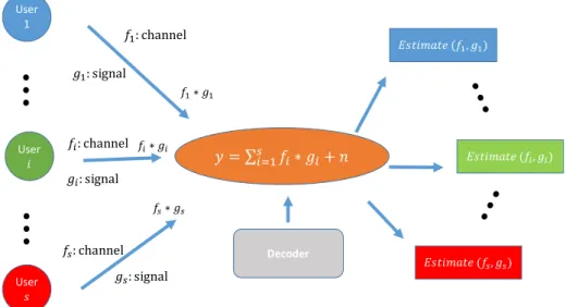
Focusing on the underlying mathematical challenges, we consider a multi-user
communica-tionscenario where many different users/devices communicate with a common base station, as
illustrated in Figure 1. Suppose we have susers and each of them sends a signal gi through an
unknown channel (which differs from user to user) to a common base station,. We assume that
∗
The authors acknowledge support from the NSF via grants DTRA-DMS 1322393 and DMS 1620455.
†
Courant Institute of Mathematical Sciences, New York University (Email: [email protected]).
‡
thei-th channel, represented by its impulse response fi, does not change during the
transmis-sion of the signalgi. Therefore fi acts as convolution operator, i.e., the signal transmitted by
thei-th user arriving at the base station becomes fi∗gi, where “∗” denotes convolution. The
User 1 User 𝑖 User 𝑠 𝑔$: signal
⋮
⋮
𝑦 = ∑5 𝑓1∗ 𝑔1+ 𝑛 16$ 𝑔1: signal 𝑔5: signal 𝑓1: channel 𝑓$: channel 𝑓5: channel 𝐸𝑠𝑡𝑖𝑚𝑎𝑡𝑒 (𝑓$, 𝑔$) 𝐸𝑠𝑡𝑖𝑚𝑎𝑡𝑒 (𝑓1, 𝑔1) 𝐸𝑠𝑡𝑖𝑚𝑎𝑡𝑒 (𝑓5, 𝑔5) Decoder 𝑓1∗ 𝑔1 𝑓$∗ 𝑔$ 𝑓5∗ 𝑔5Figure 1: Single-antenna multi-user communication scenario without explicit channel estima-tion: Each of thesusers sends a signalgi through an unknown channelfito a common base
sta-tion. The base station measures the superposition of all those signals, namely,y=Ps
i=1fi∗gi
(plus noise). The goal is to extract all pairs of {(fi,gi)}si=1 simultaneously from y.
antenna at the base station, instead of receiving each individual componentfi∗gi, is only able
to record the superposition of all those signals, namely,
y=
s
X
i=1
fi∗gi+n, (1.1)
wherenrepresents noise. We aim to develop a fast algorithm to simultaneously extract all pairs {(fi,gi)}is=1fromy(i.e., estimating the channel/impulse responsesfi and the signalsgi jointly)
in a numerically efficient and robust way, while keeping the number of required measurements as small as possible.
1.1 State of the art and contributions of this paper
A thorough theoretical analysis concerning the solvability of demixing problems via convex optimization can be found in [26]. There, the authors derive explicit sharp bounds and phase transitions regarding the number of measurements required to successfully demix structured signals (such as sparse signals or low-rank matrices) from a single measurement vector. In principle we could recast the blind deconvolution/demixing problem as the demixing of a sum of rank-one matrices, see (2.3). As such, it seems to fit into the framework analyzed by McCoy and Tropp. However, the setup in [26] differs from ours in a crucial manner. McCoy and Tropp consider as measurement matrices (see the matricesAiin (2.3)) full-rank random matrices, while
in our setting the measurement matrices are rank-one. This difference fundamentally changes the theoretical analysis. The findings in [26] are therefore not applicable to the problem of joint blind deconvolution/demixing. The compressive principal component analysis in [42] is also a form of demixing problem, but its setting is only vaguely related to ours. There is a large amount of literature on demixing problems, but the vast majority does not have a “blind deconvolution component”, therefore this body of work is only marginally related to the topic of our paper.
Blind deconvolution/demixing problems also appear in convolutional dictionary learning, see e.g. [2]. There, the aim is to factorize an ensemble of input vectors into a linear combination of overcomplete basis elements which are modeled as shift-invariant—the latter property is why the factorization turns into a convolution. The setup is similar to (1.1), but with an additional penalty term to enforce sparsity of the convolving filters. The existing literature on convolutional dictionary learning is mainly focused on empirical results, therefore there is little overlap with our work. But it is an interesting challenge for future research to see whether the approach in this paper can be modified to provide a fast and theoretically sound solver for the sparse convolutional coding problem.
There are numerous papers concerned with blind deconvolution/demixing problems in the area of wireless communications [31, 37, 20]. But the majority of these papers assumes the availability of multiple measurement vectors, which makes the problem significantly easier. Those methods however cannot be applied to the case of a single measurement vector, which is the focus of this paper. Thus there is essentially no overlap of those papers with our work.
Our previous paper [23] solves (1.1) under subspace conditions, i.e., assuming that both fi
and gi belong to known linear subspaces. This contributes to generalizing the pioneering work
by Ahmed, Recht, and Romberg [1] from the “single-user” scenario to the “multi-user” scenario. Both [1] and [23] employ a two-step convex approach: first “lifting” [9] is used and then the lifted version of the original bilinear inverse problems is relaxed into a semi-definite program. An improvement of the theoretical bounds in [23] was announced in [29].
While the convex approach is certainly effective and elegant, it can hardly handle large-scale problems. This motivates us to apply a nonconvex optimization approach [8, 21] to this blind-deconvolution-blind-demixing problem. The mathematical challenge, when using non-convex methods, is to derive a rigorous convergence framework with conditions that are competitive with those in a convex framework.
In the last few years several excellent articles have appeared on provably convergent noncon-vex optimization applied to various problems in signal processing and machine learning, e.g., matrix completion [17, 16, 34], phase retrieval [8, 11, 33, 3], blind deconvolution [19, 4, 21], dictionary learning [32], super-resolution [12] and low-rank matrix recovery [35, 41]. In this paper we derive the first nonconvex optimization algorithm to solve (1.1) fast and with rigorous theoretical guarantees concerning exact recovery, convergence rates, as well as robustness for
noisy data. Our work can be viewed as a generalization of blind deconvolution [21] (s= 1) to
the multi-user scenario (s >1).
The idea behind our approach is strongly motivated by the nonconvex optimization algo-rithm for phase retrieval proposed in [8]. In this foundational paper, the authors use a two-step approach: (i) Construct a good initial guess with a numerically efficient algorithm; (ii) Starting with this initial guess, prove that simple gradient descent will converge to the true solution. Our paper follows a similar two-step scheme. However, the techniques used here are quite different from [8]. Like the matrix completion problem [7], the performance of the algorithm relies heavily and inherently on how much the ground truth signals are aligned with the design matrix. Due to this so-called “incoherence” issue, we need to impose extra constraints, which results in a dif-ferent construction of the so-calledbasin of attraction. Therefore, influenced by [17, 34, 21], we add penalty terms to control the incoherence and this leads to the regularized gradient descent method, which forms the core of our proposed algorithm.
To the best of our knowledge, our algorithm is the first algorithm for the blind deconvolu-tion/blind demixing problem that is numerically efficient, robust against noise, and comes with rigorous recovery guarantees.
1.2 Notation
For a matrix Z, kZk denotes its operator norm and kZkF is its the Frobenius norm. For a
vectorz,kzk is its Euclidean norm andkzk∞ is the `∞-norm. For both matrices and vectors,
Z∗ and z∗ denote their complex conjugate transpose. ¯z is the complex conjugate of z. We
given vector z, diag(z) represents the diagonal matrix whose diagonal entries are z. For any
z∈R, let z+ = z+2|z|.
2
Preliminaries
Obviously, without any further assumption, it is impossible to solve (1.1). Therefore, we impose the following subspace assumptions throughout our discussion [1, 23].
• Channel subspace assumption: Each finite impulse response fi ∈ CL is assumed to have maximum delay spreadK, i.e.,
fi= hi 0 .
Here hi∈CK is the nonzero part of fi and fi(n) = 0 for n > K.
• Signal subspace assumption: Let gi := Cix¯i be the outcome of the signal ¯xi ∈ CN
encoded by a matrix Ci ∈ CL×N with L > N, where the encoding matrix Ci is known
and assumed to have full rank1.
Remark 2.1. Both subspace assumptions are common in various applications. For instance in wireless communications, the channel impulse response can always be modeled to have finite support (or maximum delay spread, as it is called in engineering jargon) due to the physical properties of wave propagation [14]; and the signal subspace assumption is a standard feature
found in many current communication systems [14], including CDMA where Ci is known as
spreading matrix and OFDM where Ci is known as precoding matrix.
The specific choice of the encoding matrices Ci depends on a variety of conditions. In this
paper, we derive our theory by assuming that Ci is a complex Gaussian random matrix, i.e.,
each entry in Ci is i.i.d. CN(0,1). This assumption, while sometimes imposed in the wireless
communications literature, is somewhat unrealistic in practice, due to the lack of a fast algorithm
to apply Ci and due to storage requirements. In practice one would rather choose Ci to be
something like the product of a Hadamard matrix and a diagonal matrix with random binary entries. We hope to address such more structured encoding matrices in our future research. Our numerical simulations (see Section 4) show no difference in the performance of our algorithm for either choice.
Under the two assumptions above, the model actually has a simpler form in the frequency
domain. We assume throughout the paper that the convolution of finite sequences is circular
convolution2. By applying the Discrete Fourier Transform DFT) to (1.1) along with the two
assumptions, we have 1 √ LF y= s X i=1 diag(F hi)(F Cix¯i) + 1 √ LF n
where F is the L×L normalized unitary DFT matrix with F∗F = F F∗ = IL. The noise
is assumed to be additive white complex Gaussian noise with n∼ CN(0, σ2d20IL) where d0 =
pPs
i=1khi0k2kxi0k2, and {(hi0,xi0)}si=1 is the ground truth. We define di0 =khi0x
∗
i0kF and assume without loss of generality that khi0k and kxi0k are of the same norm, i.e., khi0k =
kxi0k=
√
di0, which is due to the scaling ambiguity3. In that way, σ12 actually is a measure of SNR (signal to noise ratio).
1
Here we use the conjugate ¯xi instead ofxi because it will simplify our notation in later derivations.
2This circular convolution assumption can often be reinforced directly (for example in wireless communications
the use of a cyclic prefix in OFDM renders the convolution circular) or indirectly (e.g. via zero-padding). In the first case replacing regular convolution by circular convolution does not introduce any errors at all. In the latter case one introduces an additional approximation error in the inversion which is negligible, since it decays exponentially for impulse responses of finite length [30].
3
Let hi ∈CK be the first K nonzero entries of fi and B ∈ CL×K be a low-frequency DFT
matrix (the first K columns of anL×L unitary DFT matrix). Then a simple relation holds,
F fi =Bhi, B∗B=IK.
We also denoteAi:=F Ci ande:= √1LF n. Due to the Gaussianity,Ai also possesses complex
Gaussian distribution and so does e. From now on, instead of focusing on the original model,
we consider (with a slight abuse of notation) the following equivalent formulation throughout our discussion: y= s X i=1 diag(Bhi)Aixi+e, (2.1) where e∼ CN(0,σ2d20
L IL). Our goal here is to estimate all {hi,xi} s
i=1 from y,B and {Ai}si=1. Obviously, this is a bilinear inverse problem, i.e., if all {hi}si=1 are given, it is a linear inverse problem (the ordinary demixing problem) to recover all{xi}si=1, and vice versa. We note that there is a scaling ambiguity in all blind deconvolution problems that cannot be resolved by any reconstruction method without further information. Therefore, when we talk about exact recovery in the following, then this is understood modulo such a trivial scaling ambiguity.
Before proceeding to our proposed algorithm we introduce some notation to facilitate a more convenient presentation of our approach. Let bl be the l-th column of B∗ and ail be the l-th
column of A∗i. Based on our assumptions the following properties hold:
L X l=1 blb∗l =IK, kblk2= K L, ail ∼ CN(0,IN).
Moreover, inspired by the well-knownlifting idea [9, 1, 6, 22], we define the useful matrix-valued linear operatorAi:CK×N →CL and its adjointA∗i :CL→CK×N by
Ai(Z) :={b∗lZail}Ll=1, A∗i(z) := L
X
l=1
zlbla∗il=B∗diag(z)Ai (2.2)
for each 1 ≤i≤s under canonical inner product over CK×N. Therefore, (2.1) can be written in the following equivalent form
y=
s
X
i=1
Ai(hix∗i) +e. (2.3)
Hence, we can think of y as the observation vector obtained from taking linear measurements
with respect to a set of rank-1 matrices {hix∗i}si=1. In fact, with a bit of linear algebra (and ignoring the noise term for the moment), the l-th entry of y in (2.3) equals the inner product of two block-diagonal matrices:
yl= * h1,0x∗1,0 0 · · · 0 0 h2,0x∗2,0 · · · 0 .. . ... . .. ... 0 0 · · · hs0x∗s0 | {z } defined asX0 , bla∗1l 0 · · · 0 0 bla∗2l · · · 0 .. . ... . .. ... 0 0 · · · bla∗sl + +el, (2.4) where yl=Psi=1b∗lhi0x ∗
i0ail+el,1≤l≤L and X0 is defined as the ground truth matrix. In
other words, we aim to recover such a block-diagonal matrix X0 from L linear measurements
with block structure if e=0.
By stacking all {hi}si=1 (and{xi}si=1,{hi0}si=1,{xi0}si=1) into a long column, we let
h:= h1 .. . hs , h0:= h1,0 .. . hs0 ∈C Ks, x:= x1 .. . xs , x0 := x1,0 .. . xs0 ∈C N s. (2.5)
We defineHas a bilinear operator which maps a pair (h,x)∈CKs×
CN s into a block diagonal matrix inCKs×N s, i.e., H(h,x) := h1x∗1 0 · · · 0 0 h2x∗2 · · · 0 .. . ... . .. ... 0 0 · · · hsx∗s ∈CKs×N s. (2.6)
Let X := H(h,x) and X0 := H(h0,x0) where X0 is the ground truth as illustrated in (2.4). Define A(Z) :CKs×N s →CL as A(Z) := s X i=1 Ai(Zi), (2.7)
where Z = blkdiag(Z1,· · · ,Zs) and blkdiag is the standard MATLAB function to construct
block diagonal matrix. Therefore, A(H(h,x)) = Ps
i=1Ai(hix∗i) and y = A(H(h0,x0)) +e. The adjoint operatorA∗ is defined naturally as
A∗(z) := A∗1(z) 0 · · · 0 0 A∗2(z) · · · 0 .. . ... . .. ... 0 0 · · · A∗s(z) ∈CKs×N s, (2.8)
which is a linear map fromCLtoCKs×N s.To measure the approximation error ofX0 given by X, we defineδ(h,x) as the global relative error:
δ(h,x) := kX−X0kF kX0kF = q Ps i=1khix ∗ i −hi0x ∗ i0k2F d0 = s Ps i=1δ2id2i0 Ps i=1d2i0 , (2.9)
whereδi:=δi(hi,xi) is the relative error within each component:
δi(hi,xi) :=
khix∗i −hi0x∗i0kF
di0
.
Note that δ and δi are functions of (h,x) and (hi,xi) respectively and in most cases, we just
simply use δ and δi if no possibility of confusion exists.
2.1 Convex versus nonconvex approaches
As indicated in (2.4), joint blind deconvolution-demixing can be recast as the task to recover
a rank-sblock-diagonal matrix from linear measurements. In general, such a low-rank matrix
recovery problem is NP-hard. In order to take advantage of the low-rank property of the
ground truth, it is natural to adopt convex relaxation by solving a convenient nuclear norm minimization program, i.e.,
min s X i=1 kZik∗, s.t. s X i=1 Ai(Zi) =y. (2.10)
The question of when the solution of (2.10) yields exact recovery is first answered in our
previous work [23]. Late, [29, 15] have improved this result to the near-optimal bound L ≥
C0s(K+N) up to some log-factors where the main theoretical result is informally summarized in the following theorem.
Theorem 2.2 (Theorem I.1 in [15]). Suppose that Ai are L×N i.i.d. complex Gaussian
matrices and B is an L×K partial DFT matrix with B∗B = IK. Then solving (2.10) gives
exact recovery if the number of measurements L yields
L≥Cγs(K+N) log3L
with probability at least 1−L−γ where C
While the SDP relaxation is definitely effective and has theoretic performance guarantees, the computational costs for solving an SDP already become too expensive for moderate size problems, let alone for large scale problems. Therefore, we try to look for a more efficient nonconvex approach such as gradient descent, which hopefully is also reinforced by theory. It
seems quite natural to achieve the goal by minimizing the following nonlinear least squares
objective function with respect to (h,x)
F(h,x) :=kA(H(h,x))−yk2= s X i=1 Ai(hix∗i)−y 2 . (2.11) In particular, if e=0,we write F0(h,x) := s X i=1 Ai(hix∗i −hi0x∗i0) 2 . (2.12)
As also pointed out in [21], this is a highly nonconvex optimization problem. Many of the commonly used algorithms, such as gradient descent or alternating minimization, may not necessarily yield convergence to the global minimum, so that we cannot always hope to obtain the desired solution. Often, those simple algorithms might get stuck in local minima.
2.2 The basin of attraction
Motivated by several excellent recent papers of nonconvex optimization on various signal pro-cessing and machine learning problem, we propose our two-step algorithm: (i) Compute an initial guess carefully; (ii) Apply gradient descent to the objective function, starting with the carefully chosen initial guess. One difficulty of understanding nonconvex optimization consists in how to construct the so-called basin of attraction, i.e., if the starting point is inside this basin of attraction, the iterates will always stay inside the region and converge to the global minimum. The construction of the basin of attraction varies for different problems [8, 3, 34]. For this problem, similar to [21], the construction follows from the following three observations.
Each of these observations suggests the definition of a certain neighborhood and the basin of
attraction is then defined as the intersection of these three neighborhood sets Nd∩ Nµ∩ N.
1. Ambiguity of solution: in fact, we can only recover (hi,xi) up to a scalar since (αhi, α−1xi)
and (hi,xi) are both solutions for α 6= 0. From a numerical perspective, we want to avoid
the scenario when khik →0 and kxik → ∞while khikkxikis fixed, which potentially leads
to numerical instability. To balance both the norm of khik and kxik for all 1 ≤ i≤ s, we
define Nd:={{(hi,xi)}si=1:khik ≤2 p di0,kxik ≤2 p di0,1≤i≤s}, which is a convex set.
2. Incoherence: the performance depends on how large/small the incoherenceµ2h is, whereµ2h
is defined by µ2h := max 1≤i≤s LkBhi0k2∞ khi0k2 .
The idea is that: the smaller the µ2h is, the better the performance is. Let us consider an extreme case: ifBhi0is highly sparse or spiky, we lose much information on those zero/small entries and cannot hope to get satisfactory recovered signals. In other words, we need the ground truthhi0has “spectral flatness” andhi0is not highly localized on the Fourier domain. A similar quantity is also introduced in the matrix completion problem [7, 34]. The largerµ2h
is, the morehi0 is aligned with one particular row of B.To control the incoherence between bl andhi, we define the second neighborhood,
Nµ:={{hi}si=1:
√
LkBhik∞≤4 p
di0µ,1≤i≤s}, (2.13)
3. Close to the ground truth: we also want to construct an initial guess such that it is close to the ground truth, i.e.,
N := {(hi,xi)}si=1 :δi = khix∗i −hi0x∗i0kF di0 ≤ε,1≤i≤s (2.14) whereεis a predetermined parameter in (0,151].
Remark 2.3. To ensure δi ≤ε, it suffices to ensure δ ≤ √εsκ where κ := maxminddi0i0 ≥1. This is
because 1 sκ2 s X i=1 δi2 ≤δ2 ≤ ε 2 sκ2
which implies max1≤i≤sδi≤ε.
Remark 2.4. When we say (h,x) ∈ Nd,Nµ or N, it means for all i = 1, . . . , s we have
(hi,xi) ∈ Nd, Nµ or N respectively. In particular,(h0,x0)∈ Nd∩ Nµ∩ N where h0 and x0 are defined in (2.5).
2.3 Objective function and Wirtinger derivative
To implement the first two observations, we introduce the regularizer G(h,x), defined as the
sum ofscomponents G(h,x) := s X i=1 Gi(hi,xi). (2.15)
For each component Gi(hi,xi), we let ρ ≥d2+ 2kek2, 0.9d0 ≤d≤1.1d0, 0.9di0 ≤di ≤1.1di0 for all 1≤i≤sand
Gi:=ρ h G0 k hik2 2di +G0 k xik2 2di | {z } Nd + L X l=1 G0 L|b∗lhi|2 8diµ2 | {z } Nµ i , (2.16)
whereG0(z) = max{z−1,0}2. Here bothdand{di}si=1are data-driven and well approximated by our spectral initialization procedure; andµ2 is a tuning parameter which could be estimated if we assume a specific statistical model for the channel (for example, in the widely used Rayleigh fading model, the channel coefficients are assumed to be complex Gaussian). The idea behind
Gi is quite straightforward though the formulation is complicated. For each Gi in (2.16), the
first two terms try to force the iterates to lie in Nd and the third term tries to encourage the iterates to lie in Nµ. What about the neighborhood N? A proper choice of the initialization followed by gradient descent which keeps the objective function decreasing will ensure that the iterates stay inN.
Finally, we consider the objective function as the sum of nonlinear least squares objective functionF(h,x) in (2.11) and the regularizerG(h,x),
e
F(h,x) :=F(h,x) +G(h,x). (2.17)
Note that the input of the function Fe(h,x) consists of complex variables but the output is
real-valued. As a result, the following simple relations hold
∂Fe ∂h¯i = ∂Fe ∂hi , ∂Fe ∂x¯i = ∂Fe ∂xi .
Therefore, to minimize this function, it suffices to consider only the gradient of Fe with
respect to ¯hi and ¯xi, which is also called Wirtinger derivative [8]. The Wirtinger derivatives of
F(h,x) and G(h,x) w.r.t. ¯hi and ¯xi can be easily computed as follows
∇Fhi =A ∗ i (A(X)−y)xi =A∗i (A(X−X0)−e)xi, (2.18) ∇Fxi = (A ∗ i (A(X)−y)) ∗ hi = (A∗i(A(X −X0)−e))∗hi, (2.19) ∇Ghi = ρ 2di h G00 k hik2 2di hi+ L 4µ2 L X l=1 G00 L|b∗lhi|2 8diµ2 blb∗lhi i , (2.20) ∇Gxi = ρ 2di G00 k xik2 2di xi, (2.21) whereA(X) =Ps
i=1Ai(hix∗i) and A∗ is defined in (2.8). In short, we denote
∇Feh:=∇Fh+∇Gh, ∇Fh:= ∇Fh1 .. . ∇Fhs , ∇Gh:= ∇Gh1 .. . ∇Ghs . (2.22)
Similar definitions hold for ∇Fex,∇Fx and Gx. It is easy to see that ∇Fh= A∗(A(X)−y)x
and ∇Fx = (A∗(A(X)−y))∗h.
3
Algorithm and Theory
3.1 Two-step algorithm
As mentioned before, the first step is to find a good initial guess (u(0),v(0))∈CKs×CN s such that it is inside the basin of attraction. The initialization follows from this key fact:
E(A∗i(y)) =E A ∗ i s X j=1 Aj(hj0x∗j0) +e =hi0x∗i0, where we use B∗B=PL l=1blb ∗ l =IK,E(aila ∗ il) =IN and E(A∗iAi(hi0x∗i0)) = L X l=1 blb∗lhi0x∗i0E(aila∗il) =hi0x∗i0, E(A∗jAi(hi0x∗i0)) = L X l=1 blb∗lhi0x∗i0E(aila∗jl) =0, ∀j 6=i.
Therefore, it is natural to extract the leading singular value and associated left and right singular vectors from each A∗i(y) and use them as (a hopefully good) approximation to (di0,hi0,xi0). This idea leads to Algorithm 1, the theoretic guarantees of which are given in Section 6.5. The second step of the algorithm is just to apply gradient descent to Fe with the initial guess
{(u(0)i ,vi(0), di)}si=1 or (u(0),v(0),{di}si=1), where u(0) stems from stacking allu(0)i into one long
vector4.
Remark 3.1. For Algorithm 2, we can rewrite each iteration into
u(t) =u(t−1)−η∇Feh(u(t−1),v(t−1)), v(t)=v(t−1)−η∇Fex(u(t−1),v(t−1)),
where ∇Feh and ∇Fex are in (2.22), and
u(t) := u(1t) .. . u(st) , v (t):= v1(t) .. . vs(t) . 4
It is clear that instead of gradient descent one could also use a second-order method to achieve faster convergence at the tradeoff of increased computational cost per iteration. The theoretical convergence analysis for a second-order method will require a very different approach from the one developed in this paper.
Algorithm 1 Initialization via spectral method and projection 1: for i= 1,2, . . . , sdo
2: Compute A∗i(y).
3: Find the leading singular value, left and right singular vectors of A∗i(y), denoted by (di,hˆi0,xˆi0).
4: Solve the following optimization problem for 1≤i≤s:
u(0)i := argminz∈ CKkz− p dihˆi0k2 s.t. √ LkBzk∞≤2 p diµ. 5: Set v(0)i =√dixˆi0. 6: end for 7: Output: {(u(0)i ,v(0)i , di)}is=1 or (u(0),v(0),{di}si=1).
Algorithm 2 Wirtinger gradient descent with constant stepsizeη
1: Initialization: obtain (u(0),v(0),{di}si=1) via Algorithm 1.
2: for t= 1,2, . . . ,do 3: for i= 1,2, . . . , s do 4: u(it)=ui(t−1)−η∇Fehi(u (t−1) i ,v (t−1) i ), 5: vi(t) =vi(t−1)−η∇Fexi(u (t−1) i ,v (t−1) i ), 6: end for 7: end for 3.2 Main results
Our main findings are summarized as follows: Theorem 3.2 shows that the initial guess given
by Algorithm 1 indeed belongs to the basin of attraction. Moreover, di also serves as a good
approximation of di0 for each i. Theorem 3.3 demonstrates that the regularized Wirtinger
gradient descent will guarantee the linear convergence of the iterates and the recovery is exact in the noisefree case and stable in the presence of noise.
Theorem 3.2. The initialization obtained via Algorithm 1 satisfies (u(0),v(0))∈ √1 3Nd \ 1 √ 3Nµ \ N 2ε 5√sκ (3.1) and 0.9di0 ≤di ≤1.1di0, 0.9d0 ≤d≤1.1d0, (3.2)
holds with probability at least 1−L−γ+1 if the number of measurements satisfies
L≥Cγ+log(s)(µ2h+σ2)s2κ4max{K, N}log2L/ε2. (3.3)
Here ε is any predetermined constant in (0,151], and Cγ is a constant only linearly depending
onγ withγ ≥1.
Theorem 3.3. Starting with the initial valuez(0):= (u(0),v(0))satisfying (3.1),the Algorithm 2 creates a sequence of iterates (u(t),v(t)) which converges to the global minimum linearly,
kH(u(t),v(t))− H(h0,x0)kF ≤ εd0 √ 2sκ2(1−ηω) t/2+ 60√skA∗ (e)k (3.4)
with probability at least 1−L−γ+1 where ηω=O((sκd0(K+N) log2L)−1) and
kA∗(e)k ≤C0σd0
s
γs(K+N)(log2L)
L
if the number of measurements L satisfies
Remark 3.4. Our previous work [23] shows that the convex approach via semidefinite program-ming (see (2.10)) requires L ≥ C0s2(K+µ2hN) log3(L) to ensure exact recovery. Later, [15]
improves this result to the near-optimal bound L≥C0s(K+µ2hN) up to some log-factors. The difference between nonconvex and convex methods lies in the appearance of the condition number
κ in (3.5). This is not just an artifact of the proof—empirically we also observe that the value of κ affects the convergence rate of our nonconvex algorithm, see Figure 5.
Remark 3.5. Our theory suggests s2-dependence for the number of measurements L, although numericallyLin fact depends onslinearly, as shown in Section 4. The reason fors2-dependence will be addressed in details in Section 5.2.
Remark 3.6. In the theoretical analysis, we assume thatAi (or equivalentlyCi) is a Gaussian
random matrix. Numerical simulations suggest that this assumption is clearly not necessary. For example, Ci may be chosen to be a Hadamard-type matrix which is more appropriate and
favorable for communications.
Remark 3.7. If e =0, (3.4) shows that (u(t),v(t)) converges to the ground truth at a linear rate. On the other hand, if noise exists, (u(t),v(t))is guaranteed to converge to a point within a small neighborhood of(h0,x0).More importantly, if the number of measurementsL gets larger,
kA∗(e)k decays at the rate of O(L−1/2).
4
Numerical simulations
In this section we present a range of numerical simulations to illustrate and complement different aspects of our theoretical framework. We will empirically analyze the number of measurements needed for perfect joint deconvolution/demixing to see how this compares to our theoretical bounds. We will also study the robustness for noisy data. In our simulations we use Gaussian encoding matrices, as in our theorems. But we also try more realistic structured encoding matrices, that are more reminiscent of what one might come across in wireless communications.
While Theorem 3.3 says that the number of measurements L dependsquadratically on the
number of sourcess, numerical simulations suggest near-optimal performance. Figure 2
demon-strates that L actually depends linearly on s, i.e., the boundary between success (white) and
failure (black) is approximately a linear function of s. In the experiment, K = N = 50 are
fixed, all Ai are complex Gaussians and all (hi,xi) are standard complex Gaussian vectors.
For each pair of (L, s), 25 experiments are performed and we treat the recovery as a success
if kXˆ−X0kF
kX0kF ≤10
−3.For our algorithm, we use backtracking to determine the stepsize and the iteration stops either if kA(H(h(t+1),x(t+1))− H(h(t),x(t)))k < 10−6kyk or if the number of iterations reaches 500. The backtracking is based on the Armijo-Goldstein condition [25]. The initial stepsize is chosen to be η= K+1N. IfFe(z(t)−η∇Fe(z(t)))>Fe(z(t)), we just divideη by
two and use a smaller stepsize.
We see from Figure 2 that the number of measurements for the proposed algorithm to succeed not only seems to depend linearly on the number of sensors, but it is actually rather close to the information-theoretic limit s(K+N). Indeed, the green dashed line in Figure 2, which represents the empirical boundary for the phase transition between success and failure corresponds to a line with slope about 32s(K+N). It is interesting to compare this empirical performance to the sharp theoretical phase transition bounds one would obtain via convex optimization [10, 26]. Considering the convex approach based on lifting in [23], we can adapt the theoretical framework in [10] to the blind deconvolution/demixing setting, but with one modification. The bounds in [10] rely on Gaussian widths of tangent cones related to the
measurement matrices Ai. Since simply analytic formulas for these expressions seem to be
out of reach for the structured rank-one measurement matrices used in our paper, we instead compute the bounds for full-rank Gaussian random matrices, which yields a sharp bound of
about 3s(K +N) (the corresponding bounds for rank-one sensing matrices will likely have a
the empirical behavior of convex methods. Thus our empirical bound for using a non-convex methods compares rather favorably with that of the convex approach.
s: 1 to 8
Number of measurements: L, from 100 to 1250
L vs. s, K = N = 50, Regularized GD, Gaussian 1 2 3 4 5 6 7 8 250 500 750 1000 1250 0 0.1 0.2 0.3 0.4 0.5 0.6 0.7 0.8 0.9 1
Figure 2: Phase transition plot for empirical recovery performance under different choices of (L, s) where K =N = 50 are fixed. Black region: failure; white region: success. The red solid line depicts the number of degrees of freedom and the green dashed line shows the empirical phase transition bound for Algorithm 2.
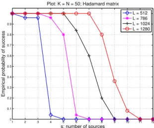
Similar conclusions can be drawn from Figure 3; there allAi are in the form ofAi =F DiH
whereF is the unitaryL×LDFT matrix, allDi are independent diagonal binary±1 matrices
andH is anL×N fixed partial deterministic Hadamard matrix. The purpose of usingDi is to
enhance the incoherence between each channel so that our algorithm is able to tell apart each individual signal and channel. As before we assume Gaussian channels, i.e., hi ∼ CN(0,IK)
Therefore, our approach does not only work for Gaussian encoding matrices Ai but also for
the matrices that are interesting to real-world applications, although no satisfactory theory has
been derived yet for that case. Moreover, due to the structure of Ai and B, fast transform
algorithms are available, potentially allowing for real-time deployment.
1 2 3 4 5 6 7 8 9 10 11 12 0 0.1 0.2 0.3 0.4 0.5 0.6 0.7 0.8 0.9 1 s: number of sources
Empirical probability of success
Plot: K = N = 50; Hadamard matrix
L = 512 L = 786 L = 1024 L = 1280
Figure 3: Empirical probability of successful recovery for different pairs of (L, s) when K =
N = 50 are fixed.
Figure 4 shows the robustness of our algorithm under different levels of noise. We also run
25 samples for each level of SNR and different Land then compute the average relative error.
It is easily seen that the relative error scales linearly with the SNR and one unit of increase in SNR (in dB) results in one unit of decrease in the relative error.
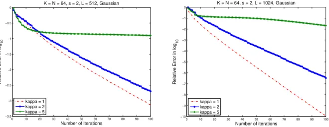
Theorem 3.3 suggests that the performance and convergence rate actually depend on the condition number of X0 = H(h0,x0), i.e., on κ = maxminddi0i0 where di0 = khi0kkxi0k. Next we
0 5 10 15 20 25 30 35 40 45 50 −60 −50 −40 −30 −20 −10 0 10 SNR(dB)
Average Relative Error of 10 Samples(dB)
K = N = 64, s = 6, Gaussian L = 2s(K+N) L = 4s(K+N) 0 5 10 15 20 25 30 35 40 45 50 −60 −50 −40 −30 −20 −10 0 10 SNR(dB)
Average Relative Error of 10 Samples(dB)
K = N = 64, s = 6, Hadamard
L = 2s(K+N) L = 4s(K+N)
Figure 4: Relative error vs. SNR (dB): SNR = 20 log10kkyekk.
demonstrate that this dependence on the condition number is not an artifact of the proof, but is indeed also observed empirically. In this experiment, we lets= 2 and set for the first component
d1,0 = 1 and for the second one d2,0 =κ for κ∈ {1,2,5}. Here, κ= 1 means that the received signals of both sensors have equal power, whereasκ= 5 means that the signal received from the second sensor is considerably stronger. The initial stepsize is chosen asη = 1, followed by the backtracking scheme. Figure 5 shows how the relative error decays with respect to the number of iterationst under different condition numberκ and L.
The largerκ is, the slower the convergence rate is, as we see from Figure 5. This may result from two reasons: our spectral initialization may not be able to give a good initial guess for those weak components; moreover, during the gradient descent procedure, the gradient directions for the weak components could be totally dominated/polluted by the strong components. Currently, we still have no effective way of how to deal with this issue of slow convergence whenκ is not small. We have to leave this topic for future investigations.
0 10 20 30 40 50 60 70 80 90 100 −3.5 −3 −2.5 −2 −1.5 −1 −0.5 0 Number of iterations
Relative Error in log
10 K = N = 64, s = 2, L = 512, Gaussian kappa = 1 kappa = 2 kappa = 5 0 10 20 30 40 50 60 70 80 90 100 −10 −9 −8 −7 −6 −5 −4 −3 −2 −1 0 Number of iterations
Relative Error in log
10
K = N = 64, s = 2, L = 1024, Gaussian
kappa = 1 kappa = 2 kappa = 5
Figure 5: Relative error vs. number of iterations t.
5
Convergence analysis
Our convergence analysis relies on the following four conditions where the first three of them are local properties. We will also briefly discuss how they contribute to the proof of our main theorem. Note that our previous work [21] on blind deconvolution is actually a special case (s= 1) of (2.1). The proof of Theorem 3.3 follows in part the main ideas in [21]. The readers may find the technical parts of [21] and this manuscript share many similarities. However,
there are also important differences. After all, we are now dealing with a more complicated
problem where the ground truth matrixX0 and measurement matrices are both rank-s
block-diagonal matrices, as shown in (2.4), instead of rank-1 matrices in [21]. The key is to understand the properties of the linear operator A applying to different types of block-diagonal matrices. Therefore, many technical details are much more involved while on the other hand, some of results in [21] can be used directly. During the presentation, we will clearly point out both the similarities to and differences from [21].
5.1 Four key conditions
Condition 5.1. Local regularity condition: Let z := (h,x) ∈ Cs(K+N) and ∇Fe(z) := " ∇Feh(z) ∇Fex(z) # ∈Cs(K+N), then k∇Fe(z)k2 ≥ω[Fe(z)−c]+ (5.1) for z∈ Nd∩ Nµ∩ N where ω= d0 7000 andc=kek 2+ 2000skA∗(e)k2.
We will prove Condition 5.1 in Section 6.3. Condition 5.1 states thatFe(z) = 0 ifk∇Fe(z)k=
0 ande= 0, i.e., all the stationary points inside the basin of attraction are global minima.
Condition 5.2. Local smoothness condition: Let z = (h,x) and w = (u,v) and there holds
kFe(z+w)−Fe(z)k ≤CLkwk (5.2)
forz+wandz insideNd∩ Nµ∩ N whereCL≈ O(d0sκ(1 +σ2)(K+N) log2L)is the Lipschitz constant ofFe over Nd∩ Nµ∩ N. The convergence rate is governed by CL.
The proof of Condition 5.2 can be found in Section 6.4.
Condition 5.3. Local restricted isometry property: Denote X = H(h,x) and X0 =
H(h0,x0). There holds 2 3kX −X0k 2 F ≤ kA(X−X0)k2≤ 3 2kX−X0k 2 F (5.3)
uniformly all for (h,x)∈ Nd∩ Nµ∩ N.
Condition 5.3 will be proven in Section 6.2. It says that the convergence of the objective function implies the convergence of the iterates.
Remark 5.4 (Necessity of inter-user incoherence). Although Condition 5.3 is seemingly the same as the one in our previous work [21], it is indeed very different. Recall that A is a linear operator acting on block-diagonal matrices and its output is the sum of s different components involvingAi. Therefore, the proof of Condition 5.3 heavily depends on the inter-user incoherence whereas this notion of incoherence is not needed at all for the single-user scenario. At the beginning of Section 2, we discuss the choice of Ci (or Ai). In order to distinguish
one user from another, it is essential to use sufficiently different5 encoding matrices Ci (or
Ai). Here the independence and Gaussianity of all Ci (or Ai) guarantee that kPTiA
∗
iAjPTjk is sufficiently small for all i6=j where Ti is defined in (6.1). It is a key element to ensure the
validity of Condition 5.3 which is also an important component to prove Condition 5.1. On the other hand, due to the recent progress on this joint deconvolution and demixing problem, one is also able to prove a local restricted isometry property with tools such as bounding the suprema of chaos processes [15] by assuming{Ai}si=1 as Gaussian matrices.
Condition 5.5. Robustness condition: Let ε≤ 1
15 be a predetermined constant. We have
kA∗(e)k= max 1≤i≤skA ∗ i(e)k ≤ εd0 10√2sκ, (5.4) where e∼ CN(0,σ2d20 L ) if L≥Cγκ 2s2(K+N)/ε2. 5
Suppose allCiare the same, there is no hope to recover all pairs of{(hi,xi)}s
We will prove Condition 5.5 in Section 6.5. We now extract one useful result based on Conditions 5.3 and 5.5. From these two conditions, we are able to produce a good approximation of F(h,x) for all (h,x)∈ Nd∩ Nµ∩ N in terms ofδ in (2.9). For (h,x)∈ Nd∩ Nµ∩ N, the
following inequality holds 2 3δ 2d2 0− εδd20 5√sκ+kek 2 ≤F(h,x)≤ 3 2δ 2d2 0+ εδd20 5√sκ +kek 2. (5.5)
Note that (5.5) simply follows from
F(h,x) =kA(X−X0)k2F −2 Re(hX−X0,A∗(e)i) +kek2. Note that (5.3) implies 23δ2d20 ≤ kA(X −X0)k2F ≤ 32δ
2d2
0. Thus it suffices to estimate the cross-term, |Re(hX −X0,A∗(e)i)| ≤ kA∗(e)kkX −X0k∗ =kA∗(e)k s X i=1 khix∗i −hi0x∗i0k∗ ≤√2kA∗(e)k s X i=1 khix∗i −hi0x∗i0kF ≤√2skA∗(e)kkX−X0kF ≤ εδd20 10√sκ (5.6)
wherek · k∗ and k · k are a pair of dual norms andkA∗(e)k comes from (5.4).
5.2 Outline of the convergence analysis
For the ease of proof, we introduce another neighborhood: N e F = (h,x) :Fe(h,x)≤ ε2d20 3sκ2 +kek 2 .
Moreover, another reason to considerN
e
F is based on the fact that gradient descentonly allows
one to make the objective function decrease if the step size is chosen appropriately. In other words, all the iterates z(t) generated by gradient descent are insideN
e
F as long asz
(0) ∈ N
e
F.
On the other hand, it is crucial to note that the decrease of the objective function does not necessarily imply the decrease of the relative error of the iterates. Therefore, we want to construct an initial guess in N∩ N
e
F so that z
(0) is sufficiently close to the ground truth and then analyze the behavior of z(t).
In the rest of this section, we basically try to prove the following relation: 1 √ 3Nd∩ 1 √ 3Nµ∩ N5√2εsκ | {z } Initial guess ⊂ N∩ NFe | {z } {z(t)} t≥0 inN∩N e F ⊂ Nd∩ Nµ∩ N | {z }
Key conditions hold overNd∩Nµ∩N
.
Now we give a more detailed explanation of the relation above, which constitutes the main structure of the proof:
1. We will show √1 3Nd∩ 1 √ 3Nµ∩ N5√2εsκ ⊂ N∩ N e
F in the proof of Theorem 3.3 in Section 5.3,
which is quite straightforward.
2. Lemma 5.6 explains why it holds thatN∩NFe ⊂ Nd∩Nµ∩Nand where thes2-bottleneck
comes from.
3. Lemma 5.8 implicitly shows that the iterates z(t) will remain in N ∩ NFe if the initial
guessz(0) is insideN∩N
e
F andFe(z(t)) is monotonically decreasing (simply by induction).
Lemma 5.9 makes this observation explicit by showing thatz(t)∈ N∩NFeimpliesz
(t+1) :=
z(t) −η∇Fe(z(t)) ∈ N ∩ N
e
F if the stepsize η obeys η ≤
1
CL. Moreover, Lemma 5.9
guarantees sufficient decrease of Fe(z(t)) in each iteration, which paves the road towards
Remember thatNdandNµare both convex sets, and the purpose of introducing regularizers
Gi(hi,xi) is to approximately project the iterates onto Nd∩ Nµ.Moreover, we hope that once
the iterates are insideN and inside a sublevel subsetNFe, they will never escape fromNFe∩ N.
Those ideas are fully reflected in the following lemma.
Lemma 5.6. Assume 0.9di0≤di ≤1.1di0 and0.9d0≤d≤1.1d0. There holds NFe ⊂ Nd∩ Nµ;
moreover, under Conditions 5.3 and 5.5, we haveN
e
F ∩ N⊂ Nd∩ Nµ∩ N109.
Proof: If (h,x) ∈ N/ d∩ Nµ, by the definition of G in (2.15), at least one component in G
exceeds ρG0 2di0 di . We have e F(h,x) ≥ ρG0 2di0 di ≥(d2+ 2kek2) 2di0 di −1 2 ≥ (2/1.1−1)2(d2+ 2kek2) ≥ 1 2d 2 0+kek2> ε2d20 3sκ2 +kek 2, where ρ ≥ d2+ 2kek2, 0.9d
0 ≤ d≤ 1.1d0 and 0.9di0 ≤di ≤1.1di0. This implies (h,x) ∈ N/ Fe
and henceN
e
F ⊂ Nd∩ Nµ.
Note that (h,x)∈ Nd∩ Nµ∩ N if (h,x)∈ NFe∩ N. Applying (5.5) gives
2 3δ 2d2 0− εδd20 5√sκ +kek 2≤F(h,x)≤ e F(h,x)≤ ε 2d2 0 3sκ2 +kek 2
which implies that δ≤ 9
10
ε
√
sκ.By definition ofδ in (2.9), there holds
81ε2 100sκ2 ≥δ 2= Ps i=1δi2d2i0 Ps i=1d2i0 ≥ Ps i=1δ2i sκ2 ≥ 1 sκ2 1max≤i≤sδ 2 i, (5.7)
which gives δi ≤ 109εand (h,x)∈ N9 10ε.
Remark 5.7. The s2-bottleneck comes from (5.7). If δ≤ε is small, we cannot guarantee that each δi is also smaller than ε. Just consider the simplest case when all di0 are the same: then
d20=Ps
i=1d2i0=sd2i0 and there holds
ε2 ≥δ2 = 1 s s X i=1 δi2.
Obviously, we cannot conclude that maxδi ≤ ε but only say that δi ≤
√
sε. This is why we require δ=O(√ε
s) to ensure δi ≤ε, which gives s
2-dependence in L.
Lemma 5.8. Denote z1 = (h1,x1) and z2= (h2,x2). Letz(λ) := (1−λ)z1+λz2. Ifz1∈ N
and z(λ)∈ N
e
F for allλ∈[0,1], we have z2 ∈ N.
Proof: Note that for z1 ∈ N ∩ NFe, we have z1 ∈ Nd ∩ Nµ ∩ N
9
10ε which follows from
the second part of Lemma 5.6. Now we prove z2 ∈ N by contradiction. Let us suppose
that z2 ∈ N/ and z1 ∈ N. There exists z(λ0) := (h(λ0),x(λ0)) ∈ N for some λ0 ∈ [0,1] such that max1≤i≤s
khix∗i−hi0x∗i0kF
di0 = . Therefore, z(λ0) ∈ NFe∩ N and Lemma 5.6 implies
max1≤i≤s
khix∗i−hi0x∗i0kF
di0 ≤ 9
10, which contradicts max1≤i≤s
khix∗i−hi0x∗i0kF
di0 =. Lemma 5.9. Let the stepsize η ≤ 1
CL, z
(t) := (u(t),v(t)) ∈
Cs(K+N) and CL be the Lipschitz
constant of ∇Fe(z) over Nd∩ Nµ∩ N in (5.2). If z(t) ∈ N∩ N e F, we have z (t+1) ∈ N ∩ NFe and e F(z(t+1))≤Fe(z(t))−ηk∇Fe(z(t))k2 (5.8) where z(t+1)=z(t)−η∇ e F(z(t)).
Remark 5.10. This lemma tells us that once z(t)∈ N∩ N
e
F, the next iterate z
(t+1) =z(t)−
η∇Fe(z(t)) is also inside N∩ N
e
F as long as the stepsize η ≤
1
CL. In other words, N ∩ NFe
is in fact a stronger version of the basin of attraction. Moreover, the objective function will decay sufficiently in each step as long as we can control the lower bound of the ∇Fe, which is
guaranteed by the Local Regularity Condition 5.3.
Proof: Let φ(τ) :=Fe(z(t)−τ∇Fe(z(t))),φ(0) =Fe(z(t)) and consider the following quantity:
τmax:= max{µ:φ(τ)≤Fe(z(t)),0≤τ ≤µ},
whereτmax is the largest stepsize such that the objective functionFe(z) evaluated at any point
over the whole line segment {z(t)−τFe(z(t)),0 ≤τ ≤τmax} is not greater than Fe(z(t)). Now
we will show τmax≥ C1L. Obviously, if k∇Fe(z(t))k= 0, it holds automatically.
Consider k∇Fe(z(t))k 6= 0 and assumeτmax< C1
L. First note that, d
dτφ(τ)<0 =⇒τmax>0.
By the definition of τmax, there holdsφ(τmax) =φ(0) since φ(τ) is a continuous function w.r.t.
τ. Lemma 5.8 implies
{z(t)−τ∇Fe(z(t)),0≤τ ≤τmax} ⊆ N∩ N
e
F.
Now we apply Lemma 6.20, the modified descent lemma, and obtain
e
F(z(t)−τmax∇Fe(z(t)))≤Fe(z(t))−(2τmax−CLτmax2 )kFe(z(t))k2 ≤Fe(z(t))−τmaxkFe(z(t))k2
whereCLτmax≤1.In other words,φ(τmax)≤Fe(z(t)−τmax∇Fe(z(t)))<Fe(z(t)) =φ(0)
contra-dictsφ(τmax) =φ(0).
Therefore, we conclude that τmax≥ C1
L. For anyη ≤ 1 CL, Lemma 5.8 implies {z(t)−τ∇Fe(z(t)),0≤τ ≤η} ⊆ N∩ N e F
and applying Lemma 6.20 gives
e
F(z(t)−η∇Fe(z(t)))≤Fe(z(t))−(2η−CLη2)kFe(z(t))k2≤Fe(z(t))−ηkFe(z(t))k2.
5.3 Proof of Theorem 3.3
Combining all the considerations above, we now prove Theorem 3.3 to conclude this section.
Proof: The proof consists of three parts:
Part I: Proof of z(0):= (u(0),v(0))∈ N∩ NFe. From the assumption of Theorem 3.3,
z(0) ∈ √1 3Nd \ 1 √ 3Nµ∩ N5√2εsκ .
First we show G(u(0),v(0)) = 0: for 0≤i≤sand the definition ofN
dand Nµ, ku(0)i k2 2di ≤ 2di0 3di <1, L|b ∗ lu (0) i |2 8diµ2 ≤ L 8diµ2 ·16di0µ 2 3L ≤ 2di0 3di <1, whereku(0)i k ≤ 2 √ di0 √ 3 , √ LkBu(0)i k∞≤ 4 √ di0µ √ 3 and 9 10di0≤di ≤ 11 10di0.Therefore G0 ku(0)i k2 2di ! =G0 kvi(0)k2 2di ! =G0 L|b∗lu(0)i |2 8diµ2 ! = 0
for all 1≤l≤Land G(u(0),v(0)) = 0. Forz(0)= (u(0),v(0))∈ N 2ε 5√sκ, we haveδ(z (0)) := √ Ps i=1δi2d2i0 d0 ≤ 2ε 5√sκ.By (5.5), there holds δ(z(0))≤ 2ε 5√sκ and G(u (0),v(0)) = 0, e F(u(0),v(0)) =F(u(0),v(0))≤ kek2+3 2δ 2(z(0))d2 0+ εδ(z(0))d20 5√sκ ≤ kek 2+ ε2d20 3sκ2 and hencez(0) = (u(0),v(0))∈ NTN e F.
Part II: The linear convergence of the objective function Fe(z(t)). Denote z(t) :=
(u(t),v(t)). Note that z(0) ∈ N ∩ NFe, Lemma 5.9 implies z
(t) ∈ N
∩ NFe for all t ≥ 0 by
induction if η≤ C1
L. Moreover, combining Condition 5.1 with Lemma 5.9 leads to
e F(z(t))≤Fe(z(t−1))−ηω h e F(z(t−1))−ci +, t≥1
withc=kek2+akA∗(e)k2 and a= 2000s. Therefore, by induction, we have
h e F(z(t))−c i +≤(1−ηω) h e F(z(t−1))−c i + ≤(1−ηω) th e F(z(0))−c i +≤ ε2d20 3sκ2(1−ηω) t where Fe(z(0)) ≤ ε2d2 0 3sκ2 +kek2 and h e F(z(0))−ci + ≤ 1 3sκ2ε2d20−akA∗(e)k2 + ≤ ε2d2 0 3sκ2. Now we conclude that hFe(z(t))−c i + converges to 0 linearly.
Part III: The linear convergence of the iterates (u(t),v(t)). Denote
δ(z(t)) := kH(u
(t),v(t))− H(h
0,x0)kF
d0
.
Note thatz(t)∈ N∩NFe⊆ Nd∩Nµ∩Nand overNd∩Nµ∩N, there holdsF0(z(t))≥ 23δ2(z(t))d20 which follows from Local RIP Condition in (5.3) andF0(z(t)) defined in (2.12). Moreover
e F(z(t))− kek2 ≥ F 0(z(t))−2 Re hA∗(e),H(u(0),v(0))− H(h0,x0)i ≥ 2 3δ 2(z(t))d2 0−2 √ 2skA∗(e)kδ(z(t))d0
whereG(z(t))≥0 and the second inequality follows from (5.6). There holds 2 3δ 2(z(t))d2 0−2 √ 2skA∗(e)kδ(z(t))d0−akA∗(e)k2≤ h e F(z(t))−c i + ≤ ε2d20 3sκ2(1−ηω) t and equivalently, δ(z(t))d0− 3√2 2 kA ∗(e)k 2 ≤ ε 2d2 0 2sκ2(1−ηω) t+ 3 2a+ 9 2 kA∗(e)k2.
Solving the inequality above forδ(z(t)), we have
δ(z(t))d0 ≤ εd0 √ 2sκ2(1−ηω) t/2+ 3 √ 2 2 + r 3 2a+ 9 2 ! kA∗(e)k ≤ √εd0 2sκ2(1−ηω) t/2+ 60√skA∗(e)k (5.9) wherea= 2000s.Letd(t) := q Ps i=1ku (t) i k2kv (t)
i k2 fort∈Z≥0.By (5.9) and triangle inequality, we immediately obtain|d(t)−d0| ≤ √εd2sκ02(1−ηω)
6
Proof of the four conditions
This section is devoted to proving the four key conditions introduced in Section 5. The local
smoothness condition and therobustness condition are relatively less challenging to deal with. The more difficult part is to show thelocal regularity condition and thelocal isometry property.
The key to solve those problems is to understand how the vector-valued linear operator A
in (2.7) behaves on block-diagonal matrices, such asH(h,x),H(h0,x0) andH(h,x)−H(h0,x0).
In particular, when s = 1, all those matrices become rank-1 matrices, which have been well
discussed in our previous work [21].
First of all, we define the linear subspaceTi⊂CK×N along with its orthogonal complement for 1≤i≤sas Ti :={Zi ∈CK×N :Zi =hi0v∗i +uix∗i0, ui∈CK,vi ∈CN}, Ti⊥:= IK− hi0h∗i0 di0 Zi IN− xi0x∗i0 di0 :Zi ∈CK×N (6.1) wherekhi0k=kxi0k= √
di0.In particular,hi0xi∗0∈Ti for all 1≤i≤s.
The proof also requires us to consider block-diagonal matrices whose i-th block belongs to
Ti (orTi⊥). LetZ = blkdiag(Z1,· · ·,Zs)∈CKs×N s be a block-diagonal matrix and sayZ ∈T if
T :={blkdiag({Zi}is=1)|Zi ∈Ti}
and Z∈T⊥ if
T⊥:={blkdiag({Zi}is=1)|Zi ∈Ti⊥}
where both T and T⊥ are subsets inCKs×N s andH(h0,x0)∈T.
Now we take a closer look at a special case of block-diagonal matrices, i.e., H(h,x) and calculate its projection onto T and T⊥ respectively and it suffices to consider PTi(hix
∗
i) and
PT⊥
i (hix
∗
i). For each blockhix∗i and 1≤i≤s, there are unique orthogonal decompositions
hi :=αi1hi0+ ˜hi, x:=αi2xi0+ ˜xi, (6.2)
where hi0 ⊥h˜i and xi0 ⊥x˜i. It is important to note that αi1 =αi1(hi) =
hhi0,hii
di0 and αi2 =
αi2(xi) =
hxi0,xii
di0 and thusαi1 andαi2 are functions ofhi andxi respectively. Immediately, we have the following matrix orthogonal decomposition forhix∗i onto Ti and Ti⊥,
hix∗i −hi0x∗i0 = (αi1αi2−1)hi0x∗i0+αi2h˜ixi∗0+αi1hi0x˜∗i | {z } belong toTi + h˜ix˜∗i | {z } belongs toT⊥ i (6.3)
where the first three components are in Ti while ˜hix˜∗i ∈Ti⊥.
6.1 Key lemmata
From the decomposition in (6.2) and (6.3), we want to analyze how k˜hik, kx˜ik, αi1 and αi2 depend onδi=
khix∗i−hi0x∗i0kF
di0 ifδi<1. The following lemma answers this question, which can
be viewed as an application of singular value/vector perturbation theory [40] applied to rank-1 matrices. From the lemma below, we can see that ifhix∗i is close to hi0x∗i0, thenPT⊥
i (hix
∗
i) is
in fact very small (of orderO(δi2di0)).
Lemma 6.1. (Lemma 5.9 in [21])Recall thatkhi0k=kxi0k=
√
di0. Ifδi :=
khix∗i−hi0x∗i0kF
di0 < 1, we have the following useful bounds
|αi1| ≤
khik
khi0k
and kh˜ik ≤ δi 1−δi khik, kx˜ik ≤ δi 1−δi kxik, kh˜ikkx˜ik ≤ δ2i 2(1−δi) di0. Moreover, ifkhik ≤2 √ di0and √ LkBhik∞≤4µ √ di0, i.e.,hi∈ NdTNµ, we have √ LkBi˜hik∞≤ 6µ√di0.
Now we start to focus on several results related to the linear operator A.
Lemma 6.2. (Operator norm of A). For A defined in (2.7), there holds
kAk ≤ps(Nlog(N L/2) + (γ+ logs) logL) (6.4)
with probability at least 1−L−γ.
Proof: Note thatAi(Zi) :={b∗lZiail}Ll=1 in (2.2). Lemma 1 in [1] implies
kAik ≤
p
Nlog(N L/2) +γ0logL
with probability at least 1−L−γ0.By taking the union bound over 1≤i≤s, maxkAik ≤
p
Nlog(N L/2) + (γ+ logs) logL
with probability at least 1−sL−γ−logs≥1−L−γ.
For Adefined in (2.7), applying the triangle inequality gives
kA(Z)k= s X i=1 Ai(Zi) ≤ s X i=1 kAikkZikF ≤ max 1≤i≤skAik v u u ts s X i=1 kZik2F = √ smax 1≤i≤skAikkZkF
whereZ = blkdiag(Z1,· · ·,Zs)∈CKs×N s.Therefore,
kAk ≤√smax
1≤i≤skAik ≤
p
s(Nlog(N L/2) + (γ+ logs) logL)
with probability at least 1−L−γ.
Lemma 6.3. (Restricted isometry property forAonT). The linear operatorArestricted onT is well-conditioned, i.e.,
kPTA∗APT − PTk ≤
1
10 (6.5)
where PT is the projection operator from CKs×N s onto T, given L≥Cγs2max{K, µ2hN}log2L
with probability at least 1−L−γ.
Remark 6.4. Here APT andPTA∗ are defined as
APT(Z) = s X i=1 Ai(PTi(Zi)), PTA ∗(z) = blkdiag(P T1(A ∗ 1(z)),· · ·,PTs(A ∗ s(z)))
respectively where Z is a block-diagonal matrix and z∈CL.
As shown in the remark above, the proof of Lemma 6.3 depends on the properties of both PTiA∗
iAiPTi and PTiA
∗
iAjPTj for i 6= j. Fortunately, we have already proven related results in [23] which are written as follows:
Lemma 6.5 (Inter-user incoherence, Corollary 5.3 and 5.8 in [23]). There hold
kPTiA ∗ iAjPTjk ≤ 1 10s, ∀i6=j; kPTiA ∗ iAiPTi− PTik ≤ 1 10s, ∀1≤i≤s (6.6)
with probability at least 1−L−γ+1 ifL≥C
Note that kPTiA∗
iAjPTjk ≤ 1
10s holds because of independence between each individual
random Gaussian matrixAi. In particular, ifs= 1, the inter-user incoherencekPTiA
∗
iAjPTjk ≤ 1
10s is not needed at all. With (6.6), it is easy to prove Lemma 6.3.
Proof of Lemma 6.3. For any block diagonal matrix Z = blkdiag(Z1,· · · ,Zs) ∈ CKs×N s and Zi ∈CK×N, hZ,PTA∗APT(Z)− PT(Z)i= X 1≤i,j≤s hAiPTi(Zi),AjPTj(Zj)i − kPT(Z)k 2 F = s X i=1 hZi,PTiA ∗ iAiPTi(Zi)− PTi(Zi)i+ X i6=j hAiPTi(Zi),AjPTj(Zj)i. (6.7) Using (6.6), the following two inequalities hold,
|hZi,PTiA ∗ iAiPTi(Zi)− PTi(Zi)i| ≤ kPTiA ∗ iAiPTi− PTikkZik 2 F ≤ kZik2F 10s , |hAiPTi(Zi),AjPTj(Zj)i| ≤ kPTiA ∗ iAjPTjkkZikFkZjkF ≤ kZikFkZjkF 10s .
After substituting both estimates into (6.7), we have
|hZ,PTA∗APT(Z)− PT(Z)i| ≤ X 1≤i,j≤s kZikFkZjkF 10s ≤ 1 10s s X i=1 kZikF !2 ≤ kZk 2 F 10 .
Finally, we show how Abehaves when applied to block-diagonal matrices X =H(h,x). In
particular, the calculations will be much simplified for the case s= 1.
Lemma 6.6. (A restricted on block-diagonal matrices with rank-1 blocks).
Consider X =H(h,x) and σmax2 (h,x) := max 1≤l≤L s X i=1 |b∗lhi|2kxik2. (6.8) Conditioned on (6.4), we have kA(X)k2 ≤ 4 3kXk 2 F+ 2 q 2skXk2
Fσ2max(h,x)(K+N) logL+ 8sσmax2 (h,x)(K+N) logL, (6.9)
uniformly for any h ∈ CKs and x ∈
CN s with probability at least 1− 1γexp(−s(K+N)) if
L≥Cγs(K+N) logL. HerekXk2F =kH(h,x)k2F =
Ps
i=1khik2kxik2.
Remark 6.7. Here are a few more explanations and facts aboutσ2max(h,x). Note thatkA(X)k2 is the sum of L sub-exponential6 random variables, i.e.,
kA(X)k2 = L X l=1 s X i=1 b∗lhix∗iail 2 . (6.10)
Here σmax2 (h,x) corresponds to the largest expectation of all those components in kA(X)k2. Forσmax2 (h,x), without loss of generality, we assumekxik= 1for1≤i≤sand leth∈CKs be a unit vector, i.e.,khk2=Ps
i=1khik2 = 1. The bound 1 L ≤σ 2 max(h,x)≤ K L (6.11) 6
For the definition and properties of sub-exponential random variables, the readers can find all relevant information in [38].
follows from Lσ2max(h,x)≥PL
l=1
Ps
i=1|b∗lhi|2 =khk2= 1.
Moreover, σ2
max(h,x) andσmax(h,x) are both Lipschitz functions w.r.t. h.Now we want to determine their Lipschitz constants. First note that for kxik= 1, σmax(h,x) equals
σmax(h,x) = max
1≤l≤Lk(Is⊗b
∗
l)hk
where ⊗ denotes Kronecker product. Let u∈CKs be another unit vector and we have
|σmax(h,x)−σmax(u,x)|= max 1≤l≤Lk(Is⊗b ∗ l)h−1max≤l≤Lk(Is⊗b∗l)uk = max 1≤l≤L|k(Is⊗b ∗ l)hk − k(Is⊗b∗l)uk| ≤ max 1≤l≤Lk(Is⊗b ∗ l)(h−u)k ≤ kh−uk (6.12) where kIs⊗b∗lk=kblk q K L <1.For σ 2 max(h,x),
|σmax2 (h,x)−σmax2 (u,x)| ≤(σmax(h,x) +σmax(u,x))· |σmax(h,x)−σmax(u,x)|
≤ 2K
L kh−uk ≤2kh−uk. (6.13)
Proof of Lemma 6.6. Without loss of generality, letkxik= 1 andPsi=1khik2 = 1. It suffices
to provef(h,x)≤ 4
3 for all (h,x)∈C
Ks×
CN s in (2.5) wheref(h,x) is defined as
f(h,x) :=kA(X)k2−2p2sσ2
max(h,x)(K+N) logL−8sσ2max(h,x)(K+N) logL.
Part I: Bounds of kA(X)k2 for any fixed (h,x). From (6.10), we already know thatY =
kA(X)k2
F =
P2L
i=1ciξi2 where{ξi} are i.i.d. χ21 random variables andc = (c1,· · ·, c2L)T ∈R2L. More precisely, we can determine {ci}2i=1L as
s X i=1 b∗lhix∗ail 2 =c2l−1ξ22l−1+c2lξ22l, c2l−1 =c2l= 1 2 s X i=1 |b∗lhi|2 because Ps i=1b∗lhix∗iail∼ CN 0,Psi=1|b∗lhi|2 . By the Bernstein inequality, there holds
P(Y −E(Y)≥t)≤exp − t 2 8kck2 ∨exp − t 8kck∞ (6.14) whereE(Y) =kXk2F = 1.In order to apply the Bernstein inequality, we need to estimatekck2 and kck∞as follows, kck∞= 1 21max≤l≤L s X i=1 |b∗lhi|2= 1 2σ 2 max(h,x), kck2 2= 1 2 L X l=1 s X i=1 |b∗lhi|2 2 ≤ 1 2 s X i=1 L X l=1 |b∗lhi|2 ! max 1≤l≤L s X i=1 |b∗lhi|2≤ 1 2σ 2 max(h,x). Applying (6.14) gives P(kA(X)k2≥1 +t)≤exp − t 2 4σ2 max(h,x) ∨exp − t 4σ2 max(h,x) . In particular, by setting t=g(h,x) := 2p2sσ2
max(h,x)(K+N) logL+ 8sσ2max(h,x)(K+N) logL, we have
P kA(X)k2 ≥1 +g(h,x)≤e−2s(K+N)(logL).
So far, we have shown that f(h,x)≤1 with probability at least 1−e−2s(K+N)(logL) for a fixed pair of (h,x).
Part II: Covering argument. Now we will use a covering argument to extend this result for all (h,x) and thus prove thatf(h,x)≤ 4
3 uniformly for all (h,x).
We start with defining K and Ni as 0-nets of SKs−1 and SN−1 for h and xi,1 ≤ i ≤ s,
respectively. The bounds |K| ≤ (1 + 2
0)
2sK and |N
i| ≤ (1 + 20)2N follow from the covering
numbers of the sphere (Lemma 5.2 in [38]). Here we let N := N1 × · · · × Ns. By taking the
union bound overK × N,we have thatf(h,x)≤1 holds uniformly for all (h,x)∈ K × N with probability at least
1−(1 + 2/0)2s(K+N)e−2s(K+N) logL= 1−e−2s(K+N)(logL−log(1+2/ε0)). For any (h,x) ∈ SKs−1× SN−1× · · · × SN−1
| {z }
stimes
, we can find a point (u,v) ∈ K × N satisfying
kh−uk ≤ε0 and kxi−vik ≤ε0 for all 1≤i≤s. Conditioned on (6.4), we know that
kAk2≤s(Nlog(N L/2) + (γ+ logs) logL)≤s(N +γ+ logs) logL.
Now we aim to evaluate |f(h,x)−f(u,v)|. First we consider |f(u,x)−f(u,v)|. Since
σmax2 (u,x) =σ2max(u,v) if kxik=kvik=kuk= 1 for 1≤i≤s, we have
|f(u,x)−f(u,v)| = kA(H(u,x))k 2 F − kA(H(u,v))k 2 F ≤ kA(H(u,x−v))k · kA(H(u,x+v))k ≤ kAk2 v u u t s X i=1 kuik2kxi−vik2 v u u t s X i=1 kuik2kxi+vik2
≤ 2kAk2ε0≤2s(N+γ+ logs)(logL)ε0
where the first inequality is due to ||z1|2− |z2|2| ≤ |z1−z2||z1+z2|for any z1, z2 ∈C. We proceed to estimate |f(h,x)−f(u,x)|by using (6.13) and (6.12),
|f(h,x)−f(u,x)| ≤ J1+J2+J3
≤ (2kAk2+ 2p2s(K+N) logL+ 16s(K+N) logL)ε0
≤ 25s(K+N+γ+ logs)(logL)ε0
where (6.13) and (6.12) give
J1 = kA(H(h,x))kF2 − kA(H(u,x))k2F ≤ kA(H(h−u,x))k kA(H(h+u,x))k ≤2kAk2ε0, J2 = 2 p
2s(K+N) logL· |σmax(h,x)−σmax(u,x)| ≤2
p
2s(K+N) logLε0,
J3 = 8s(K+N)(logL)· |σ2max(h,x)−σmax2 (u,x)| ≤16s(K+N)(logL)ε0.
Therefore, if 0= 81s(N+K+γ1+logs) logL, there holds
f(h,x)≤f(u,v) +|f(u,x)−f(u,v)|+|f(h,x)−f(u,x)|
| {z }
≤27s(K+N+γ+logs)(logL)ε0≤13
≤ 4
3
for all (h,x) uniformly with probability at least 1−e−2s(K+N)(logL−log(1+2/ε0)). By letting
L ≥ Cγs(K+N) logL with Cγ reasonably large and γ ≥ 1, we have logL−log (1 + 2/ε0) ≥ 1
2(1 + log(γ)) and with probability at least 1− 1
γexp(−s(K+N)).
6.2 Proof of the local restricted isometry property
Lemma 6.8. Conditioned on (6.5)and (6.9), the following RIP type of property holds: 2 3kX −X0k 2 F ≤ kA(X−X0)k2≤ 3 2kX−X0k 2 F
uniformly for all (h,x) ∈ Nd∩ Nµ∩ N with µ≥µh and ≤ 151 if L≥Cγµ2s(K+N) log2L
Proof: The main idea of the proof follows two steps: decompose X −X0 onto T and T⊥, then apply (6.5) and (6.9) to PT(X −X0) andPT⊥(X −X0) respectively.
For anyX =H(h,x)∈ N withδi ≤ε≤ 151, we can decompose X−X0 as the sum of two block diagonal matricesU = blkdiag(Ui,1≤i≤s) andV = blkdiag(Vi,1≤i≤s) where each
pair of (Ui,Vi) corresponds to the orthogonal decomposition ofhix∗i −hi0x∗i0, hix∗i −hi0x∗i0 := (αi1αi2−1)hi0x∗i0+αi2h˜ixi∗0+αi1hi0x˜∗i | {z } Ui∈Ti + ˜hix˜∗i | {z } Vi∈Ti⊥ (6.15)
which has been briefly discussed in (6.2) and (6.3). Note that A(X −X0) =A(U +V) and
kA(U)k − kA(V)k ≤ kA(U+V)k ≤ kA(U)k+kA(V)k.
Therefore, it suffices to have a two-side bound for kA(U)k and an upper bound for kA(V)k
whereU ∈T andV ∈T⊥ in order to establish the local isometry property.
Estimation of kA(U)k: ForkA(U)k, we know from Lemma 6.3 that
r 9 10kUkF ≤ kA(U)k ≤ r 11 10kUkF (6.16)
and hence we only need to compute kUkF.By Lemma 6.1, there also hold kVikF ≤ δ
2 i 2(1−δi)di0 and δi− kVikF ≤ kUikF ≤δi+kVikF, i.e., δi− δi2 2(1−δi) di0 ≤ kUikF ≤ δi+ δ2i 2(1−δi) di0, 1≤i≤s. With kUk2 F = Ps i=1kUik2F, it is easy to get δd0 1− ε 2(1−ε) ≤ kUkF ≤ δd0 1 +2(1ε−ε). Combined with (6.16), we get
r 9 10 1− ε 2(1−ε) δd0≤ kA(U)k ≤ r 11 10 1 + ε 2(1−ε) δd0. (6.17)
Estimation of kA(V)k: Note that V is a block-diagonal matrix with rank-1 block. So applying Lemma 6.6 gives us
kA(V)k2≤ 4 3kVk 2 F + 2 q 2skVk2
Fσmax2 (˜h,x˜)(K+N) logL+ 8sσmax2 (˜h,x˜)(K+N) logL (6.18) whereV =H(˜h,x˜) and ˜h= ˜ h1 .. . ˜ hs
.It suffices to get an estimation of kVkF and σ
2
max(˜h,x˜) to
boundkA(V)kin (6.18).
Lemma 6.1 says that k˜hikkx˜ik ≤ δ
2 i 2(1−δi)di0 ≤ ε 2(1−ε)δidi0 ifε <1. Moreover, kx˜ik ≤ δi 1−δi kxik ≤ 2δi 1−δi p di0, √ LkBh˜ik∞≤6µ p di0, 1≤i≤s (6.19) if (h,x) belongs to Nd∩ Nµ∩ N.ForkVkF, kVkF = v u u t s X i=1 kVik2F = v u u t s X i=1 kh˜ik2kx˜ik2 ≤ εδd0 2(1−ε).