Classification of Laser and Visual Sensors Using Associative
Markov Networks
Jos´e Angelo Gurzoni Jr, Fabiano R. Correa, Fabio Gagliardi Cozman
1Escola Polit´ecnica da Universidade de S˜ao Paulo
S˜ao Paulo, SP – Brazil
{jgurzoni,fgcozman}@usp.br, [email protected]
Abstract. This work presents our initial investigation toward the semantic clas-sification of objects based on sensory data acquired from 3D laser range and cameras mounted on a mobile robot. The Markov Random Field framework is a popular model for such a task, as it uses contextual information to improve over locally independent classifiers. We have employed a variant of this framework for which efficient inference can be performed via graph-cut algorithms and dy-namic programming techniques, the Associative Markov Networks (AMNs). We report in this paper the basic concepts of the AMN, its learning and inference algorithms, as well as the feature classifiers that serve to extract meaningful properties from sensory data. The experiments performed with a publicly avail-able dataset indicate the value of the framework and give insights about the next steps toward the goal of empowering a mobile robot to contextually reason about its environment.
1. Introduction
Perception is very important for autonomous robots operating in unstructured environ-ments. These robots have to rely on their perception capabilities not only for self lo-calization and mapping of potentially unknown and changing environments, but also for reasoning about the state of the tasks. Autonomous robots are also often used in oper-ations requiring real-time processing capabilities, what further constrain the solutions to the perception problem, due to the trade-off between processing time and quality of the reasoning.
In this work, we classify data collected by laser and camera sensors into object labels that can be used in semantic reasoning systems. A common classification approach for this classification problem is to learn a feature classifier that assigns a label to each point, independently of the assignment of its neighbors. However, noisy readings cause the labels to lose local consistency. Also, as adjacent points in the scans tend to have similar labels (if the data is used jointly), higher classification accuracy can be achieved [Munoz et al. 2009b] [Triebel et al. 2006] [Anguelov et al. 2005].
These facts suggest that the classifier to be used must be able to perform joint classification, and besides to be able to efficiently perform inference. Markov Random Fields offer such a framework. In this paper, we employ Associative Markov Networks [Taskar et al. 2004].
This paper is organized as follows: Sec. 2 describes related work. Sec. 3 intro-duces Associative Markov Networks, while Sec 4 describes the specifics of the developed
laser and image classifier, followed by the experimental results in Sec. 5. Finally, Sec. 6 presents conclusions gathered on this first stage of development and future directions. The data used on the experiments section is from the M´alaga Dataset [Blanco et al. 2009].
2. Related Work
Object recognition from 3D data on robotic applications is an open problem that has attracted attention of the scientific community, with many different, and often comple-mentary, approaches. For example, [Newman et al. 2006] used 3D laser scanner and loop closure detection based on photometric information to perform self-localization and au-tomatic mapping (SLAM). Several efforts have focused on feature extraction, such as [Johnson and Hebert 1999], that introduced spin images as rotation invariant features, and [Vandapel et al. 2004], that applied the expectation-maximization algorithm (EM) to learn a Gaussian Mixture classifier based on the analysis of saliency features.
[Rottmann et al. 2005] used a boosting algorithm on the vision and laser range classifier, with a Hidden Markov Model to increase the robustness of the final classifica-tion, while [Douillard et al. 2008] built maps of objects in which accurate classification is achieved by exploiting the ability of Conditional Random Fields (CRFs) to represent spatial correlations and to model the structural information contained in clusters of laser scans. In [Douillard et al. 2011], the same CRF approach used in their previous work is applied on a combination of vision and laser data sensors, with interesting results.
[Anguelov et al. 2005] used Markov Random Fields (MRFs) to incorporate knowledge of neighboring data points. The authors also applied the maximum margin approach [Taskar et al. 2004] as an alternative to the traditional maximum a posteriori (MAP) estimation used to learn the Markov network model. The maximum margin al-gorithm consists of maximizing the margin of confidence in the true label assignment of predicted classes. It provides improvements in accuracy and allows high-dimensional feature spaces to be utilized by using the kernel trick, as in support vector machines.
Markov Random Fields are indeed a popular choice for approaching the joint clas-sification problem. [Triebel et al. 2006] used the same technique as Anguelov et al.’s work, extending it to adaptively sample points from the training data, thus reducing the training times and dataset sizes. In [Munoz et al. 2009b], the authors develop algorithms to deal with Markov Random Fields consisting of high-order cliques in an efficient man-ner. [Micusik et al. 2012] also employ MRFs for learning and inference but, unlike the other cited works, their mechanism start by detecting parts of the objects for which they already have semantically annotations and then compute the likelihood of these parts forming a given object.
3. Associative Markov Networks
Associative Markov Networks (AMNs) [Taskar et al. 2004] form a sub-class of Markov Random Fields (MRFs) that can model relational dependencies between classes and for which efficient inference is possible.
Aregular MRF over discrete variables is an undirected graph(V,E)defining the joint distribution of the variables over its possible values{1, ..., K}, where the nodesV
classification task of this work, let the set of aforementioned variables be separated in two categories:Y, the vector of data labels we want to estimate, andX, the vector of features retrieved from the data. Then, a conditional MRF can have its distribution expressed as follows: P(y|x) = Q c∈Cφc(xc, yc) P y0 Q c∈Cφc(xc, yc0) , (1)
whereCis the set of cliques of the graph,φcare the clique potentials,xcare the features andyc the labels of the clique c. The clique potentials are mappings from features and labels of the clique to a non negative value expressing how well these variables fit together. Consider now apairwiseversion of the Markov Random Field, that is, a network where all cliques involve only single nodes or a pair of nodes, with edgesE ={(ij)|(i < j)}. In thispairwiseMRF, only nodes and edges are associated with potentialsϕandψ, respectively. Eq. (1) then can be arranged as in Eq. (2), whereZ is thepartitionfunction, the sum over all possible labellingsy, and a computational problem on the learning task which will need to be dealt with.
P(y|x) = 1 Z N Y i=1 ϕ(xi, yi) Y (ij)∈E ψ(xij, yi, yj), (2) whereZ =P y0 QN i=1ϕ(xi, yi0) QN (ij)∈Eψ(xij, yi0, yj0).
The maximum a posteriori (MAP) inference problem in a Markov Random Field is to findarg maxyP(y|x).
From the pairwise MRF shown in Eq. (2), it is possible to define an Associative Markov Network with the addition of restrictions encoding the situations where variables may have the same value. In this work, restrictions are applied only on the edge potential ψ, as they are meant to act on relations between nodes, penalizing assignments where ad-jacent nodes have different labels (as in [Triebel et al. 2006] and [Anguelov et al. 2005]). To achieve that, the constraintswk,l
e = 0 fork 6= l andwk,ke ≥ 0are added, resulting in ψ(xij, k, l) = 1fork6=landψ(xij, k, k) = λkij, withλkij ≥1.
The simplest model to define theϕandψpotentials is thelog-linearmodel, where weight vectorswkandwk,lare added to the potentials, which, using the same notation of [Triebel et al. 2006], becomes
logϕ(xi, yi) = K X k=1 (wkn·xi)yki, (3) logψ(xij, yi, yj) = K X k=1 (wk,le ·xij)ykiy l j, (4) where the indicator variableyk
i is1when pointpihas labelkand0otherwise. Then, using the log-linear model and substituting (3) and (4) in (2) results in
logPw(y|x) = N X i=1 K X k=1 (wkn·xi)yki + K X (ij)∈E K X k=1 (wek,l·xij)yiky l j −logZw(x). (5)
To learn the weightsw, one can maximize logPw(ˆy|x). However, as the parti-tion funcparti-tion Z depends on the weightsw, the operation would involve performing the intractable calculation of Z for each w. However, if the maximization is performed on the margin between the optimal labeling yˆ and any other labeling y, defined by
logPw(ˆy|x)−logPw(y|x), the term Zw(x)on (5) can be canceled, because it does not depend on the labelsy, and the computation will be efficient. This method is referred to as maximum margin optimization.
The maximum margin problem can be reduced to a quadratic program (QP), as algebraically described on [Taskar et al. 2004]. Here, for simplicity, we only mention that this quadratic program has the form:
min1 2kwk 2 +ξ (6) s.t. wXyˆ−N +ξ≥ N X i=1 αi; we≥0; αi− X ij,ji∈E αkij ≥wkn·xi−yˆik, ∀i, k; αkij +αkji≥wke ·xij, αkij, α k ji ≥0 ∀ij ∈E, k;
whereξ is a slack variable representing the total energy difference between the optimal and achieved solutions. The α are regularization terms. For K = 2, the binary clas-sifier, there is an exact solution capable of producing the optimalsolution, whereas for K >2, an approximate solution is available, as detailed in [Taskar et al. 2004]. We also recommend the reading of [Anguelov et al. 2005] for this purpose.
The next section will present the implemented solution, with feature classifiers connected to the described AMN model.
4. Feature Extraction and Object Detection
Before the Associative Markov Network can detect objects from sensors, it is desirable to perform dimensionality reduction on the several thousands of data points, and a common approach to this goal is to add preprocessing and feature extraction stages to the process. The data preprocessing normally consists of merging the different sensors’ data (an op-eration calledregistration), aligning them according to a common reference frame and properly accounting for the movement of the robot between readings. Once the data is properly preprocessed, features are extracted by a set of classifiers constructed to detect discriminative aspects of the data. It should be noted that the classifiers used in this work for feature extraction were, to a good extent, taken from [Douillard et al. 2011].
Preprocessing of multi-sensor data is not a trivial task, as sensors operate asyn-chronously and are mounted at different positions. Also, different sensors often have
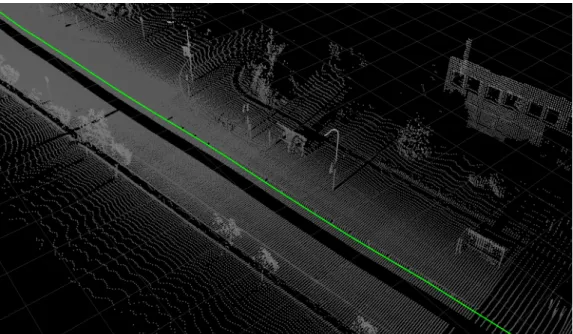
Figure 1. Sample 3D point cloud resulting from the registration of the two vertical SICK laser scanners mounted on the vehicle used in [Blanco et al. 2009]. The solid green line shows the traveled path.
different data rates, as is the case between laser scanners and cameras. When merging the information, both spatial and temporal alignment need to be performed. In this work, the use of the M´alaga Dataset [Blanco et al. 2009] (sample shown in Fig. 1) alleviated the computation of registration tasks, as the authors of the dataset provide ground truth, sensor calibration information and already registered versions of laser scanner data. What remained to be done was to project the camera images onto the 3D laser scan data, an op-eration also described in [Blanco et al. 2009], but that, in this work, was performed only in regions of interest and in a later stage to avoid processing of useless data.
Once data is preprocessed, the feature extraction phase starts. Similarly to [Douillard et al. 2011], the initial operation consists of generating the elevation map, us-ing the frame coordinates present in the laser scan data, and classifyus-ing what parts repre-sent the ground of the terrain, an information that can be used to reference thez axis of the potential objects.
The ground classifier employed is rather straightforward: a grid map with cells of a fixed size of 2 x 2 m is set (the size was chosen empirically), and the height values of all cells are computed as the difference between the maximum and minimum height values of the laser scan points that belong to the same cell. If the cell has an object on it, it must present this difference larger than a certain value, indicating the height of the object. In this work, the empirical fixed value of 30 cm was used as the threshold. A difference larger than the threshold causes the cell to be marked as having a potential object, otherwise it is marked as empty.
After the ground classifier execution, a clustering algorithm merges the neighbor cells marked as being potential objects, resulting in an object candidate list. This algo-rithm also averages the height on all the ground cells surrounding the object clusters listed and marks the computed value as thez axis reference of that object candidate. As of now,
this algorithm performs a full scan on the grid, and has not been optimized in any form. A more efficient implementation is certainly needed.
At this stage, the result is data grouped in two broad classes, ground and object candidates. The remaining classifiers operate on the object candidate class. As this work is a preliminary investigation, the attempt was to use only some classifiers, cited in the literature as being significantly discriminative, to better understand them. The normal practice in the robotics community is to employ several classifiers, some of them very specific to the problem in question. The use of large number of classifiers is justified by the need to reach very high classification results, sometimes above90%.
4.1. Feature Extractors
For the joint classification of laser scanner and image features, a set of classifiers, called of feature extractors, evaluate geometric as well as visual information present on the data. These classifiers are listed and briefly described ahead, followed by the description of the AMN learning and inference methods that use the extracted features.
• Histograms of Oriented Gradients
The HOG descriptor [Dalal and Triggs 2005] is reported to be useful in detecting pedestrians. It is a shape-based detector that represents the orientation histogram of the image contained in the data point. It relies on the idea that object appearance and shape can often be characterized by the distribution of local intensity gradients or edge directions. Its implementation is based on the creation of cell regions and creating the histograms of gradient directions or edge orientations within the cell. In the implemented version of the algorithm, the histogram values are output to eight angular bins, representing the normalized orientation distribution.
• HSV Color Histogram
This descriptor extracts HSV color information from the data point image projec-tion, filling eight bins. Therefore, these bins describe the intensity levels of 8 color tones on the data point.
• Ki Descriptor
The Ki Descriptor, developed by [Douillard 2009], captures the distinctive vertical profile of the objects. Using the ground level information added during the ground removal preprocessing as reference, the z axis is discretized into parts of 5 cm height. Then, horizontal rectangles are fitted to the points which fall into each level and the length of rectangles’ edges are measured and their values stored.
• Directional Features
Based on the implementation by [Munoz et al. 2009b], this extractor obtains ge-ometry features present on the laser range data. It estimates the local tangent vt and normalvnvectors for each point through the principal and smallest eigenvec-tors of M, respectively, and then computes the sine and cosine of the directions of vtandvnin relation to thexandzplanes, resulting in four values. At last, the con-fidence level of the features is estimated with the normalization of the values based on the strength of the extracted directions:{vt, vn}by{σl, σs}/max(σl, σp, σs). 4.2. Pairwise AMN Applied to Object Detection
The core of the implemented object detection algorithm is the pairwise AMN model. As described in Sec. 3, the model contains two potential functions, the ϕpotential in Eq.
(3) for the nodes and theψ potential in Eq. (4) for the edges of the graph. These poten-tial functions are formed by the feature vectorsxi andxij, which represent the features describing node iand edge (i, j), respectively, multiplied by the node and edge weight vectorswnandwe, formed by the concatenation of the different weights associated with features extracted from data.
For the particular task of object detection on laser range and image data, nodes of the AMN represent data points and edges represent the similarity relations between nodes, in this work given by their spatial proximity. Adata pointis defined as a set of 3D laser scan points and their associated image projection contained in a cube of 0.4 m3 (We note here that the simple cubic segmentation employed on this early stage investigation is inefficient and must be replaced).
The purpose of the AMN in the system is to label data points into the classescar, tree,pedestrianorbackground, where background represents everything not in the other classes. The task is formulated as a supervised learning task: given manually annotated training sets, the system learns the weight vectors, which are later used to classify new and unlabeled data points. The learning phase consists of solving the QP program in (6), a computationally intensive process that took hours on a computer with the Intel i7 processor executing the IBM ILOG CPLEX Studio QP solver.
After the weights are learned, inference on unlabeled data can be performed. This phase highlights an advantage of the max-margin solution for AMNs. As max-margin learning does not require computation of marginals, inference can be performed in real-time, either with a linear program or with a graph-cut algorithm. The implemented system uses a graph-cut solution proposed by [Boykov and Kolmogorov 2004], the min-cut aug-mented with iterative alpha-expansion. (from the implementation on the M3N library by
[Munoz et al. 2009a]). This version of the min-cut is guaranteed to find the optimal so-lution for binary classifiers (K = 2) and also guarantees a factor 2 approximation for K ≥2.
5. Experiments
The dataset used for the experiments of this paper is the M´alaga dataset [Blanco et al. 2009], collected at the Teatinos Campus of the University of M´alaga (Spain), however it is worth to mention the MRPT project 1 and the Robotic 3D Scan Repository of Osnabruck and Jacobs universities2, which contain other useful datasets.
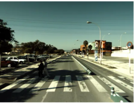
The car used was equipped with 3 SICK and 2 Hokuyo laser scanners, 2 Firewire color cameras mounted as a stereo camera, and precise navigation systems such as three RTK GPS receivers, used to generate the ground truth. Fig. 2 has a sample image from the dataset.
In this dataset, there are two data captures, collected while driving an electric golf car for distances of over 1.5 km on the streets of the university campus, at different dates. For the experiments, the trajectories of the two data captures were divided in 16 pieces of equal duration, then 4 pieces were selected as training data and labels were manually annotated. The annotation procedure consisted of drawing cubic bounding boxes marking
1http://www.mrpt.org/
Figure 2. Sample image of the camera mounted on the car - from the Malaga dataset.
the start and end frames where the labeling should occur, using the log player visualization screen. Between the start and end frames, a linear interpolation of the bounding box position accounted for the object’s movement. As this sort of interpolation inevitably introduces noise, the solution was to perform new markings every few dozens of frames. Nevertheless, this procedure was of significant help on the task of annotating the large amount of data.
Having the training set, the learning phase was performed, as described in Sec. 4.2. Using IBM CPLEX solver on a computer with an Intel i7 quad processor and 8GB RAM memory, the process took something between 2.5 and 3 hours.
With the weight vectors adjusted on the learning phase, we proceeded to the core of the experiment, the inference of the unlabeled data in the remaining 12 pieces of the datasets. Each of the dataset pieces was played, and data points of 0.4 m3 cubic size
were retrieved from it, using a simple 3D grid algorithm. As mentioned earlier, should be noted that the grid algorithm is inefficient, taking almost 1 second for each laser scan to be processed. As existing literature has several examples of algorithms suited for real-time, for now we disregarded the performance bottleneck caused by this algorithm. We plan to replace it, though, in future work.
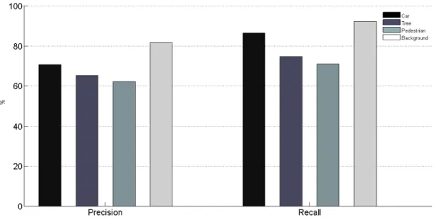
With the data points extracted, the min-cut with alpha expansion algorithm was performed, using 3-fold cross validation. Fig. 3 shows precision and recall values result-ing from the experiment. The lower detection rate for the class pedestrian is believed to be caused by the small number of training examples found, as the datasets do not contain many instances of pedestrians captured.
Overall, the results are positive for an initial investigation, although state-of-the art research indicates detection rates bordering 90%. Some reasons for the lower performance are the set of feature extractor classifiers used, selected from intuition, and the small number of feature extractors when compared to other existing works.
Figure 3. Precision and Recall results of the classification. 3-fold cross-validation, averaged results.
6. Conclusions and Future Works
This initial investigation indicated that applications of Markov Random Fields to detection and segmentation of complex objects present a number of attractive theoretical and prac-tical properties, encouraging the continuation of the research toward the goal of reasoning on meaningful information taken from sensors of a mobile robot. The investigation also suggests that diverse, uncorrelated, classifiers tend to complement each other, achieving good results when applied together.
The results obtained with the simple set of feature extractors utilized show good results, what serves as motivation to investigate the accuracy of the classifiers found in the literature. Better understanding of the capabilities and complementarity between clas-sifiers should allow us to reach higher performance levels, closer to the state-of-the-art.
During this work, it became clear that the object detection problem on mo-bile robotic platforms is still open and has many ramifications to be explored as future work. For instance, on the algorithmic efficiency/tractability issue, [Munoz et al. 2009a] present important improvements on the learning and inference algorithms, including ef-ficient solution for networks with high-order cliques. On another avenue of research, [Teichman et al. 2011] innovate by tracking objects and exploring the additional tempo-ral information rather than working on snapshots of data.
Finally, very interesting publicly available datasets were recently released. Among them, the MIT DARPA Urban Challenge dataset [Huang et al. 2010] and the Stanford Track Collection [Teichman et al. 2011]. In future work we intend to explore the high quality data these datasets provide.
Acknowledgements
The second author is partially supported by CNPq. The work reported here has received substantial support through FAPESP grant 2008/03995-5.
The authors would like to thank all the developers of the open-source projects Robot Operating System (ROS) and Point Cloud Library (PCL), whose work has been essential for the development of this work. Thanks also to the owners of the publicly available datasets used in this work.
References
[Anguelov et al. 2005] Anguelov, D., Taskar, B., Chatalbashev, V., Koller, D., Gupta, D., Heitz, G., and Ng, A. (2005). Discriminative learning of markov random fields for segmentation of 3d range data. InConference on Computer Vision and Pattern Recog-nition (CVPR).
[Blanco et al. 2009] Blanco, J.-L., Moreno, F.-A., and Gonzalez, J. (2009). A collection of outdoor robotic datasets with centimeter-accuracy ground truth. Autonomous Robots, 27(4):327–351.
[Boykov and Kolmogorov 2004] Boykov, Y. and Kolmogorov, V. (2004). An experimental comparison of mincut/max-flow algorithms for energy minimization in vision. PAMI. [Dalal and Triggs 2005] Dalal, N. and Triggs, B. (2005). Histograms of oriented
gradi-ents for human detection. InConference on Computer Vision and Pattern Recognition (CVPR).
[Douillard 2009] Douillard, B. (2009). Laser and Vision Based Classification in Urban Environments. PhD thesis, School of Aerospace, Mechanical and Mechatronic Engi-neering of The University of Sydney.
[Douillard et al. 2008] Douillard, B., Fox, D., and Ramos, F. (2008). Laser and vision based outdoor object mapping. InProc. of Robotics: Science and Systems.
[Douillard et al. 2011] Douillard, B., Fox, D., Ramos, F. T., and Durrant-Whyte, H. F. (2011). Classification and semantic mapping of urban environments. International Journal of Robotic Research (IJRR), 30(1):5–32.
[Huang et al. 2010] Huang, A. S., Antone, M., Olson, E., Moore, D., Fletcher, L., Teller, S., and Leonard, J. (2010). A high-rate, heterogeneous data set from the DARPA urban challenge. International Journal of Robotics Research (IJRR), 29(13).
[Johnson and Hebert 1999] Johnson, A. and Hebert, M. (1999). Using spin images for effi-cient object recognition in cluttered 3d scenes. IEEE Transactions on Pattern Analysis and Machine Intelligence, 21(5):433–449.
[Micusik et al. 2012] Micusik, B., Koseck´a, J., and Singh, G. (2012). Semantic parsing of street scenes from video. International Journal of Robotics Research, 31(4):484–497. [Munoz et al. 2009a] Munoz, D., Bagnell, J. A., Vandapel, N., and Hebert, M. (2009a).
Contextual classification with functional max-margin markov networks. InIEEE Con-ference on Computer Vision and Pattern Recognition (CVPR).
[Munoz et al. 2009b] Munoz, D., Vandapel, N., and Hebert, M. (2009b). Onboard contex-tual classification of 3-d point clouds with learned high-order markov random fields. InProc. of the IEEE International Conference on Robotics and Automation (ICRA).
[Newman et al. 2006] Newman, P., Cole, D., and Ho, K. (2006). Outdoor SLAM using visual appearance and laser ranging. InProc. of the IEEE International Conference on Robotics and Automation (ICRA).
[Rottmann et al. 2005] Rottmann, A., Mart´ınez Mozos, O., Stachniss, C., and Burgard, W. (2005). Place classification of indoor environments with mobile robots using boosting. InProceedings of the AAAI Conference on Artificial Intelligence.
[Taskar et al. 2004] Taskar, B., Chatalbashev, V., and Koller, D. (2004). Learning associa-tive Markov networks. InTwenty First International Conference on Machine Learning. [Teichman et al. 2011] Teichman, A., Levinson, J., and Thrun, S. (2011). Towards 3d object recognition via classification of arbitrary object tracks. InInternational Conference on Robotics and Automation (ICRA).
[Triebel et al. 2006] Triebel, R., Kersting, K., and Burgard, W. (2006). Robust 3d scan point classification using associative Markov networks. In Proc. of the IEEE International Conference on Robotics and Automation (ICRA).
[Vandapel et al. 2004] Vandapel, N., Huber, D., Kapuria, A., and Hebert, M. (2004). Nat-ural terrain classification using 3-d lidar data. In IEEE International Conference on Robotics and Automation (ICRA).