Three Essays on Migration Economics

(1)

University of Essex

Doctoral Thesis

Three Essays on Migration Economics

Author:

Juli´anCostas-Fern´andez

Supervisor:

Dr. Ben Etheridge Prof. Matthias Parey

A thesis submitted in fulfilment of the requirements for the degree of Doctor of Philosophy

in the

Department of Economics University of Essex

(2)

(3)

iii

Declaration of Authorship

I, Juli´an Costas-Fern´andez, declare that this thesis titled, “Three Essays on

Mi-gration Economics” and the work presented in it are my own. I confirm that: • This work was done wholly or mainly while in candidature for a research degree

at this University.

• Where any part of this thesis has previously been submitted for a degree or any other qualification at this University or any other institution, this has been clearly stated.

• Where I have consulted the published work of others, this is always clearly attributed.

• Where I have quoted from the work of others, the source is always given. With the exception of such quotations, this thesis is entirely my own work.

• I have acknowledged all main sources of help.

• Where the thesis is based on work done by myself jointly with others, I have made clear exactly what was done by others and what I have contributed myself.

(4)

(5)

v

Abstract

This thesis examines the selection of immigrants and their impact on the receiving economy.

After an introductory first chapter, I present an analysis of Borjas model of se-lection extended to multiple locations. In this extension, sese-lection is determined by earnings’ dispersion alone only for the most and least disperse locations. Therefore, it highlights that, what determines selection, is the ranking of locations rather than the relative dispersion of earnings between home and destination. Using interstate US migration, I provide stochastic dominance relations on pre-migration earnings that support the implications of the model. These give a stronger test for selection than selection on means.

The third chapter presents evidence on the effect of immigrants on aggregate labour productivity in the UK. I exploit variation on past settlement of natives across industries and regions to estimate the effect of immigrants on labour productivity. My estimates show that increasing the relative supply of immigrant labour has a positive effect on labour productivity. I show that part of this effect works through accumu-lation of capital stocks and provide evidence suggesting that immigrants trigger the development of technologies that complement them. Thus, I show that altering the labour mix produces effects that go beyond simple differences in marginal products and affects the accumulation of other inputs and technologies.

In the fourth chapter, Greta Morando and I exploit cross-cohort variation within majors and universities to estimate the effect of foreign peers on native students. We show that increasing the share of EU students lowers the probability of entering a university major. But, conditional on university and major, foreign peer effects on educational and early labour market outcomes are mild. Therefore, our research shows that there are no large foreign peer effects in higher education. However, it also suggests that there is scope for foreign students affecting natives’ outcomes by shaping the universities and majors natives attend.

(6)

(7)

vii

Acknowledgements

To my parents and siblings.

I would like to thank my supervisors Ben Etheridge and Matthias Parey for their continuous support and advice. Without them the research contained in this the-sis wouldn’t have been possible. I would also like to express my deep gratitude to Myra Mohnen, Michel Serafinelli, Tim Hatton, Giovanni Mastrobuoni and Gordon Kemp. Throughout my Ph.D they were always up for a chat and my work has greatly improved thanks to them.

I have been fortunate to share my Ph.D experience with wonderful friends. I would like to thank Patri Abal-Pino, Andrea Albertazzi, Alex Alonso-Campo, Patryk Bronka, Emil Kostadinov, Simon Lodato, Greta Morando, Ipek Mumcu and Federico Vaccari. A very special thanks goes to Cristina Corredor-Bejar for her continuous support while navigating through my studies.

The research here included has been funded by the ESRC. Moreover, a substantial part of the research contained in the second chapter of this thesis was carried while working as a Ph.D intern at the Migration Advisory Committee. As such, I am deeply grateful to the MAC. Particularly, I would like to thank Alan Manning and Maria del Castillo from whom my work has greatly benefited. Finally, the research contained in the fourth chapter of this thesis is the result of my collaboration with Greta Morando. Each of us has contributed a 50% to this project.

(8)

(9)

ix

List of Figures

2.1 One-year interstate migration rate . . . 18

2.2 Moving Reason Age Profile . . . 20

2.3 Ranking of Locations . . . 24

2.4 Pre-Migration Earnings CDF . . . 27

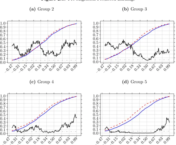
2.5 Pre-Migration Predicted Earnings . . . 30

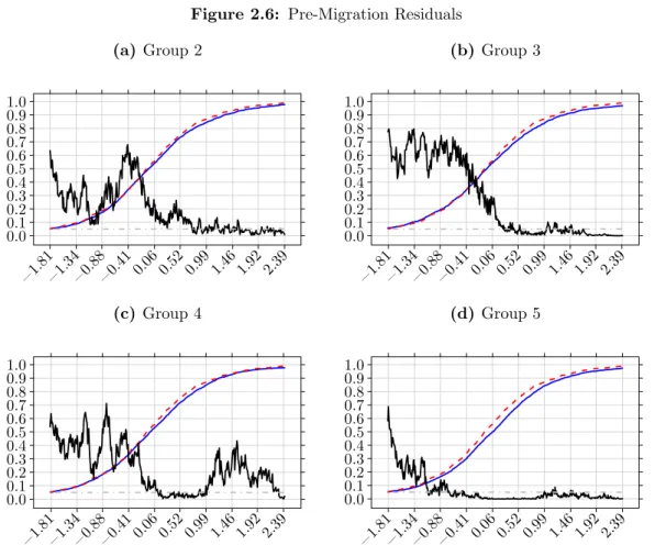
2.6 Pre-Migration Residuals . . . 31

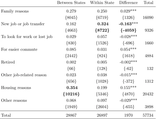
2.7 Pre-Migration Earnings CDF 25-55 Year Old . . . 40

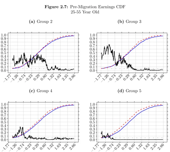
2.8 Pre-Migration Earnings CDF Males . . . 41

2.9 Pre-Migration Earnings CDF Females . . . 42

2.10 Pre-Migration Predicted Earnings 25-55 Year Old . . . 43

2.11 Pre-Migration Predicted Earnings Males . . . 44

2.12 Pre-Migration Predicted Earnings Females . . . 45

2.13 Pre-Migration Residuals 25-55 Year Old . . . 46

2.14 Pre-Migration Residuals Males . . . 47

2.15 Pre-Migration Residuals Females . . . 48

3.1 Regional Differences and Evolution . . . 58

3.2 Immigrant-Technology Regression Coefficient (atφ= 2.84) . . . 70

3.3 Relative Supply Immigrant Labour Marginal Product (atφ= 1) . . . 74

3.4 Output per Worker Evolution Regions . . . 80

3.5 Workforce Jobs and LFS: Measures of Employment . . . 81

3.6 Immigrant Stock Evolution . . . 81

3.7 Immigrant-Native Ratios (Comparison of Measures) . . . 82

3.8 Difference in Immigrant Labour Marginal Product (atφ= 1) . . . 82

4.1 Simulated International Peer Effect On Effort Provision . . . 99

4.2 Balance Test Socio-economic Background . . . 109

4.3 A10 Students Evolution . . . 132

4.4 A10 Students Evolution Between Cohorts Changes . . . 133

4.6 Sex, Age and School . . . 157

4.5 Simulated Ability Distribution . . . 158

4.7 Ethnicity . . . 159

4.8 Disability . . . 159

4.9 Share of international students by major, 2001/2010 . . . 160

(12)

4.11 Share of Foreign students by type of HEI . . . 161 4.12 Ability Density Enrolled Students . . . 162 4.13 Evolution of Foreign Students Inflows . . . 162

(13)

1

Chapter 1

Introduction

An increasingly large number of individuals live and work outside their country of birth. This has led, over the last twenty years, to the immigrant population share in developed countries doubling and reaching 14% of the total population by 2019.1 Unsurprisingly, immigration and its consequences have become a central issue for academics, policymakers and the general public.2

The economic literature has recognised the importance of migration, at least, as early as Ravenstein (1885). In the modern literature, one of the most influential papers on migration economics is Borjas (1987) work on selection of migrants. Borjas uses the occupational framework introduced by Roy (1951) and models migration decisions as an earnings maximization problem. The main implication of his model is that earnings dispersion alone determines the direction of selection. High-skilled workers move to disperse locations that give them a better chance to increase their earnings and low-skilled workers choose more equal locations to insure themselves against extreme bad earnings draws (Parey et al. 2017).

Since Borjas (1987), immigrant self-selection has received widespread attention. For example, migrant selection from Mexico to the US has been the subject of intense debate (Ambrosini and Peri 2012; Chiquiar and Hanson 2005; Fernandez-Huertas Moraga 2011; Kaestner and Malamud 2014; Orrenius and Zavodny 2005). A com-mon element to most of the migrant selection literature that followed Borjas (1987), is that it uses a two-location model. This is true even when studying migration phe-nomena where workers face multiple destinations (e.g. Belot and Hatton 2012; Borjas, Kauppinen, et al. 2018; Feliciano 2005; Fernandez-Huertas Moraga 2013; Parey et al. 2017). Borjas, Bronars, et al. (1992) is, to the best of my knowledge, the only ex-ception. In their study of interstate migration, Borjas, Bronars, et al. (1992) present a Roy model of selection with perfect transferability of skills. This perfect transfer-ability of skills simplifies the model, but it is a restriction regarding Borjas original

1

According to United Nations data.

2_{As a public issue, immigration has gained salience across the political spectrum (Dancygier and} Margalit 2019) and this, ultimately, translates into public policy (Facchini et al. 2016). For example, in the UK, immigration has played a key role in one of the UK biggest policy changes, leaving the European Union (Goodwin and Milazzo 2017). This growing interest in immigration gives a compelling argument to study its causes and consequences.

(14)

model that one may not want to impose. Particularly when studying international migration.3

In the second chapter of this thesis, I present an analysis of Borjas’ model extended to multiple locations and general transferability of skills. I show that this extension of the model predicts positive (negative) selection to the most (least) disperse loca-tion. This highlights something that gets overlooked in the two-location model, what matters for selection is the ranking of locations in terms of earnings dispersion. This is in contrast with the most common interpretation in the literature that interprets the selection mechanism as given by relative earnings dispersion between home and destination. As a result, this interpretation of the selection mechanism guides, in some way, most of the analysis framed within the Borjas model. For example, Belot and Hatton (2012) regress measures of worker quality on differences in returns to education at home and destination. And Abramitzky and Boustan (2017), in their review of immigrant selection, note that some literature (Feliciano 2005; Grogger and Hanson 2011; Jasso et al. 2004; Kennedy et al. 2015) finds positive immigrant selection to the US independently of differences between home and destination.

That the home location plays no role in selection through differences in dispersion has the following intuition. In most models of migration (e.g. Dahl 2002; Kennan and Walker 2011) the home location is defined as a preference, or location amenity, shifter. This is, the home location does not enter the earnings equation or, in any case, only displaces the location of the net earnings distribution. This is also true in Borjas’ model. Then, given that selection is driven by relative returns to skill and these are not affected by the home location, the home location must play no role in selection.

Although home location plays no special role on whether there is positive or negative selection, it affects the intensity of selection. However, this is intuitive and results from using earnings obtained at home to measure skill. To see the intuition, let me give an extreme example. Imagine that all workers are ex-ante equal, then the dispersion of earnings in the home location is zero, everyone earns the same wage, and there can be no-selection.4 If workers have heterogeneous skills, then there can be selection and the dispersion of earnings at home will be non-zero. In addition, the more heterogeneous the skills of workers are, the greater the degree of selection can be. Moreover, in the model, if one substitutes earnings at home for some other measure of skill, the effect of earnings dispersion at home on the intensity of selection disappears. This shows that the effect of home location earnings dispersion is given by how one measures skill, not the mechanism of selection.

When exploring the implications of my multiple locations Borjas’ model, I fol-low Borjas, Kauppinen, et al. (2018) and study stochastic dominance relations be-tween earnings distributions. This has two advantages when compared with selection

3

See the extensive literature on immigrant downgrading following Chiswick (1978). See also the review by Dustmann and G¨orlach (2015).

4

This is inside the one price Roy model. In other set-ups it is possible to generate wage dispersion with ex-ante identical workers (e.g. Postel-Vinay and Robin 2002).

(15)

Chapter 1. Introduction 3

on mean earnings. First, stochastic dominance relations produce simpler expres-sions when dealing with multiple locations. Second, stochastic dominance produces a stronger test for the implications of the model. This is because, first order, stochastic dominance implies ordering of means. However, the opposite is generally not true.

To test the implications of the model, I use US interstate migration. This mi-gration phenomenon gives me the best testing laboratory possible. This is because, when moving across states, workers do not face policy constraints. This is in contrast with most international migration where skill-based admission may contaminate the underlying pattern of selection.5 Moreover, interstate migrants stay within the scope of the Survey of Income and Program Participation, from where I get the data for my analysis. This avoids, or at least limits, representativeness concerns that are, otherwise, an issue on international migration (Ibarraran and Lubotsky 2007) and al-lows me to observe characteristics and earnings of movers before they move. Finally, earnings differentials across states are significant and long-lasting (Dahl 2002). Thus, there is scope for the selection mechanism described by Borjas’ model taking place.

Using the Survey of Income and Program Participation and the Current Popula-tion Survey I classify states according to their earnings dispersion and characterize immigrant selection using pre-migration earnings. The empirical evidence I provide matches quite well the selection pattern described by the model. Selection increases with earnings dispersion at the destination location. Furthermore, the earnings dis-tribution of those moving to the least disperse location never dominates the earnings distribution of other migrants and the earnings distribution of those moving to the most disperse locations is never dominated. This pattern holds for observed, predicted and residual pre-migration earnings across sex and age groups.

Alongside migrant selection, a large branch within migration economics asks what are the consequences of immigration for receiving economies.6 Earlier literature fo-cused on the effects in the receiving labour market (e.g. Borjas and Tienda 1987; Card 1990; Grossman 1982; Hunt 1992; Johnson 1980; LaLonde and Topel 1991).7 Specifi-cally, the earlier literature focused on the effect of immigrants on natives’ wages (see also Altonji and Card 1991; Borjas, Freeman, et al. 1992; Butcher and Card 1991).

Since the early 1990s, the literature has spread in terms of outcomes studied. For example, there are recent studies on the effect of immigrants on crime (Bell et al. 2013; Mastrobuoni and Pinotti 2015), attitudes towards migration (Dustmann and Preston 2007; Viskanic 2017), public services (Preston 2014; Wadsworth 2013), real-estate (S´a 2014) and education (Hunt 2017; Machin and Murphy 2017). Nonetheless, the effects of immigration on the receiving labour market are, still, the central issue (e.g. Dustmann, Fabbri, et al. 2005; Dustmann, Frattini, et al. 2013; Dustmann,

5_{There is some evidence that immigration policy has been shifting towards promoting high-skilled} immigration (see Boucher and Cerna 2014, and other papers in the same special issue.).

6_{Spengler (1958) may be one of the earliest examples of this literature.} 7

An, earlier, exception is Reder (1963). He discusses the effects of post-war immigration on investment, output per capita, labour supply and income distribution.

(16)

Sch¨onberg, et al. 2017; Hatton and Tani 2005; Manacorda et al. 2012; Ottaviano and Peri 2012).8

In the third and fourth chapters of this thesis, I contribute to this literature by estimating the effect of immigrants in two, relatively, unexplored outcomes. In my third chapter, I investigate the effect of immigrants on labour productivity in the UK. Immigration and productivity are growing concerns for British policymakers (see ministerial white papers BEIS 2017; Home Office 2018). However, there is little evidence of the effect of immigration on productivity. Aleksynska and Tritah (2009), Boubtane et al. (2016), and Ortega and Peri (2014) provide cross-country evidence showing that immigration has a positive effect on labour productivity. A similar conclusion is reached by Peri (2012) using data from the US and by Ottaviano, Peri, and Wright (2018) using service sector data for the UK. However, Paserman (2013) finds negative effects on Israeli manufacturing firms and Kangasniemi et al. (2012) provide mixed evidence for Spain and the UK.

My third chapter contributes to the literature by estimating the average effect of immigrants on labour productivity in the UK. Using variation on past-settlement of immigrants (Altonji and Card 1991; Card 2001) across regions and industries, I estimate the effect of altering the relative supply of immigrant labour on labour productivity. My estimates show that increasing the relative supply of immigrant labour by ten percentage points rises output per worker by 6.7%. Evaluated at the average, this is a£5,610 increase in annual output per worker.

To better understand the reduced-form estimate, I introduce a Constant Elastic-ity of Substitution production function which I use to decompose the reduced form estimate. I show that the reduced-form effect is composed of differences in marginal returns between immigrant and native labour and the changes immigrants induce on other inputs. Thus, a key insight from my decomposition is that reduced-form estimates of the effect of immigration on output and labour productivity depends on the mix of inputs. Therefore, it warns against extrapolating estimates across time, country, sectors or levels of aggregation as the input mix varies across these dimensions.9

To gauge the importance of effects on other inputs on the reduced form effect, I estimate the effect of immigration on capital stocks, native labour, and native skill mix. My estimates show that immigrants have a positive effect on capital stocks, native labour and native skill mix. However, the positive effect of immigration on labour productivity goes beyond effects on these inputs. Controlling for capital and native skill mix, I estimate that immigrants have a positive and significant effect on labour productivity. Increasing the relative supply of immigrant labour by ten percentage points increases labour productivity by 5%.

Given the persistence of the positive effect of immigration on labour productivity,

8

See also chapters 3 to 6 in Borjas (2014) and the review by Card and Peri (2016). 9_{See figure 3.1, table 3.1 and evidence provided by Dustmann, Sch¨}_{onberg, et al. (2016).}

(17)

I explore whether it works through differences on relative marginal returns or if im-migrants may trigger the development of technologies that complement them. Using my decomposition of the reduced form effect I show that, for a wide range of pa-rameter values, the evidence I provide is consistent with immigrants encouraging the development of technologies that complement them. This positive effect is consistent with Acemoglu (1998, 2002) model of endogenous technical change. In Acemoglu’s model, as long as immigrant and native labour are gross substitutes, increasing the relative supply of immigrant labour increases the supply of technologies that com-plement immigrants. To provide further evidence about whether this mechanism is at place, I compare estimates from two production function estimators with the reduced form effect controlling for other inputs. Assuming that factor augmenting technologies are constant, my production function estimate produces an immigrant marginal effect that is only positive when I allow for effects through capital stocks. This is in contradiction with the reduced form effect and further suggest that im-migrants have an effect on technologies that complement them. Moreover, when I compare this production function estimate with a polynomial approximation, that is consistent with endogenous technical change, I find that the approximation produces a larger and positive marginal effect. This suggests, again, that immigrants trigger the development of migrant labour augmenting technologies.

My work on the effect of immigration on labour productivity, therefore, shows that changing the labour mix produces effects that go beyond differences in marginal products and into effects through other inputs and, possibly, technologies. This fits well within the existing literature. Clemens et al. (2018) produce suggestive evidence pointing to endogenous technological change as a result of immigrant restrictions. Hornbeck and Naidu (2014) show that reductions in the availability of cheap labour lead to the introduction of technology to substitute it. Moreover, Hornung (2014) and Hunt and Gauthier-Loiselle (2010) show that immigrants can boost the diffusion and development of innovations. Finally, Hunt (2017), Llull (2017), and Ransom and Winters (2016) show that immigrants shape natives’ educational decisions.

The fourth chapter of this thesis goes, precisely, into that last effect. Do im-migrants change educational outcomes of natives? However, differently from Hunt (2017), Llull (2017), and Ransom and Winters (2016) that study the effect of changes on the aggregate stock of immigrants; Greta Morando and I ask what is the effect of sharing university and major with foreign peers on educational and early labour market outcomes of native students. Our research is motivated by an ever-growing number of international students in higher education that makes the effects of in-ternational students in the receiving country and, particularly, on native students key for policy (see MAC 2018). This is because higher education is a key stage for the future labour market performance of workers. At this stage, the universities and colleges that individuals attend (Arcidiacono 2004; Belfield et al. 2018; Walker and Zhu 2008, 2018) and the educational outcomes they achieve (Feng and Graetz 2017; Jaeger and Page 1996; Jones and Jackson 1990) have an impact on future labour

(18)

market outcomes.

There is substantial literature on the effect of peers on individuals’ outcomes.10 However, the literature on foreign peer effects is still small and has focused on lower levels of education. Ballatore et al. (2018) find negative foreign peer effects on lan-guage and math performance of second graders.11 _{In contrast with this, Geay et al.} (2013) show that, in England, the negative effect of foreign peers on natives is be-cause of selection and that foreign peers produce a zero effect. Moreover, in their study of foreign peers on Israeli natives, Gould et al. (2009) find an overall no effect that, however, hides a negative effect for disadvantaged students. Finally, Ohinata and Van Ours (2013) study the effect of foreign peers on Dutch students finding only mild effects.

At higher education, Anelli, Shih, et al. (2017) study the effect of foreign peers on the probability of graduating in a science, technology, engineering and mathematics (STEM) major at a university in California. Their evidence shows that foreign peers have a negative effect on the probability of graduating in a STEM major. However, this has no negative effect on natives’ earnings as immigrant peers displace native students into high earning social science majors. Also in the US, but using aggregate data, Orrenius and Zavodny (2015) provide evidence showing that increasing the share of immigrants in a cohort has a negative effect on the probability of STEM graduation for women. Finally, Chevalier et al. (2019) study the impact of linguistic diversity at a British university finding no effects on English-speaking students.

We add to the literature by estimating foreign peer effects in higher education on native educational and labour market outcomes for the whole of England. The main identification problem that we face is that certain institutions may attract particular native students and also attract foreign students (Ohinata and Van Ours 2013). We deal with self-selection into university and majors by using variation across cohorts within university and major. However, we show that this variation alone is not good enough to estimate the effect of foreign peers. This is because universities have ex-ante information about the quality of prospective students. Then, under capacity constraints, an increase in the number of prospective students, as given by a larger number of foreigners, increases the average ability of accepted students. We show that this is the case for EU students who share with natives the same cap on the number of subsidized students allowed to be enrolled by each university.12 This produces that rising the share of EU students increases average ability of enrolled natives. However, non-EU students have no significant effects on average native ability. The same asymmetry holds for group size. Increasing the share of EU students does not produce any change in the size of the group, but increasing the share of non-EU increases group size.

10

See Sacerdote (2011) review of the literature on education peer effects.

11_{Brunello and Rocco (2013) also provide evidence of negative effects but at the aggregate level.} 12

This was imposed by the Higher Education Funding Council for England (HEFCE) (see Machin and Murphy 2017).

(19)

Thanks to the quality of our data we can overcome this initial selection problem. This is because we observe a measure of natives’ ability, their Universities and Colleges Admissions Service (UCAS) score. We show that, after conditioning on ability and group size, variation across cohorts within university and major is uncorrelated with a large set of pre-determined individual characteristics that are likely predictors of educational achievement.

The evidence we provide shows that there are only mild foreign peer effects and that these are heterogeneous across the ability distribution. The strongest foreign peer effects that we find are on the distribution of grades, in particular, on the probability of graduating with an upper- or lower-second for top ability students. We show that these effects on grades are not consistent with a grading-on-a-curve mechanism where foreign peers mechanically displace native students. Foreign peers, therefore, modify the human capital accumulation of native students. However, these effects are very mild. For example, the largest effect we find shows that a one percentage point increase on the foreign peer share reduces the probability of graduating with an upper second for top ability natives by .30 percentage points.

In terms of early labour market outcomes, we also find mild and typically sta-tistically non-significant foreign peer effects. If anything, foreign peers increase the probability of natives working after graduation by reducing the probability of them going into further education; increase the probability of working in professional oc-cupations and have a positive impact on wages of top ability natives.

Our research, therefore, is consistent with existing evidence providing mild foreign peer effects (Anelli, Shih, et al. 2017; Chevalier et al. 2019). However, it also suggests that foreign students may have an effect on the universities and majors that natives end up attending. This can, potentially, have a greater impact than foreign peer effects.

(20)

(21)

9

Chapter 2

Selection by Destination:

Revisiting Stochastic Dominance

in the Borjas Model

(22)

(23)

11

Abstract

Since Borjas (1987) seminal paper, the Roy model has been widely used to study immigrant self-selection. Particularly, the baseline two-location model has been a popular frame for self-selection research, even in situations where immigrants may face a larger choice set. I present an analysis of Borjas’ model of selection extended to multiple locations. This extension shows that earnings dispersion alone determines selection only for the most and least disperse locations. Therefore, it highlights that, what determines selection, is the ranking of locations rather than the relative dispersion of earnings between home and destination. Using US internal migration, I provide evidence supporting the implications of the model.

(24)

2.1 Introduction

A long-standing empirical observation is that migrants are not randomly drawn from their population, they are selected in terms of their skills.

Seminal work in Borjas (1987) uses Roy (1951) occupational choice framework to explore this phenomenon. In the baseline model, individuals choose between two locations and decide where to work based on the returns to their skills and moving costs creating a selection mechanism that is entirely characterized by relative earnings dispersion or skill premium. Higher (lower) earnings dispersion at destination leads to positive (negative) selection. Thus, the selection mechanism behind this pattern can be thought of as low skilled individuals taking insurance from the more com-pressed distribution at the destination and high skilled taking advantage of improved opportunities in a more disperse location (Parey et al. 2017).

Recently, migrant selection has received renewed interest and several papers, most notably on Mexico-US migration, have tested the implications of the Borjas (1987) framework. Chiquiar and Hanson (2005) find medium to positive selection of Mexican migrants to the US, what is evidence against Borjas selection model as Mexico is a more unequal country than the US. However, later revision (Ambrosini and Peri 2012; Fernandez-Huertas Moraga 2011, 2013; Ibarraran and Lubotsky 2007; Kaestner and Malamud 2014) provide evidence supporting the implications of Borjas’ model. Outside Mexico-US, Parey et al. (2017) use data on German graduates and provide evidence supporting the implications of the model. Borjas, Kauppinen, et al. (2018) provide further evidence in support of the Borjas using Danish data.

Several papers in the literature (e.g. Belot and Hatton 2012; Feliciano 2005; Fernandez-Huertas Moraga 2013; Parey et al. 2017) use the two-location model when studying selectivity of immigrants across multiple locations. A common interpreta-tion of the main implicainterpreta-tion of the Roy model is that”if the home country’s income distribution is more unequal than in the ...[destination], immigrants will be negatively selected...” (Feliciano 2005, p. 133). This interpretation guides, in some way, most of the analysis framed within the Borjas model. For example, Belot and Hatton (2012) regress measures of educational selectivity on differences in relative returns to edu-cation between home and destination loedu-cation. My extension of the Borjas model including more than two locations highlights that selection is not driven by relative earnings dispersion between home and destination but by the ranking, in terms of earnings dispersion, of locations within the choice set. With more than two locations and unrestricted transferability of skills, my extension of the Borjas model predicts positive (negative) immigrant selection into the most (least) disperse location.

In the two-location model, the ranking and home-destination relative dispersion are equivalent and leads to the interpretation given in the literature. However, analy-sis of selection within the Borjas model looking at home-destination relative dispersion implicitly assumes that immigrants only consider these two locations. Although that could be the case in some migration phenomena, for example, Mexico-US, it can be

(25)

2.2. Theoretical Framework 13

restrictive for other where individuals are likely to decide among a wider range of alternatives. For example, US interstate migration (Kennan and Walker 2011) or emigration across European countries (Rojas-Romagosa and Bollen 2018).

Using US inter-state migration, I test whether migrant selection follows the pat-tern implied by my extension of the Borjas model. This migration phenomenon gives a perfect scenario to test the implications of the Borjas model as there are no border constraints that could contaminate the pattern of selection and individuals can be tracked even if they switch locations. This reduces measurement error, for exam-ple, due to illegal migration (Ibarraran and Lubotsky 2007), and allows observation of pre-migration characteristics. Furthermore, when engaging on internal migration, US workers face a large choice set, as highlighted by Kennan and Walker (2011), that matches well the set-up of my extension of the Borjas model. Finally, US local labour markets exhibit heterogeneity in their earnings distribution and such differences are long-lasting (Dahl 2002). Therefore, the selection drive presented in Borjas (1987) is at place.

For testing, I use data from the Survey of Income and Program Participation and Current Population Survey covering the period 1984 to 2013. Following Borjas, Kauppinen, et al. (2018), I cast the implications of the model in terms of stochastic dominance, which provides a stronger test than selection on means. In line with the model’s predictions, I show that immigrants moving to the most (least) disperse location are positively (negatively) selected in terms of pre-migration earnings and immigrants to other locations show, somehow, intermediate selection. I show, also in line with the model, that the degree of selection increases with dispersion at the home location. Thus, I contribute to the literature by showing that a multiple location Roy model without imposing perfect transferability of skills (see Borjas, Bronars, et al. 1992) holds meaningful implications, at least for the least and most disperse locations, and that the implied pattern of selection is observed in the data.

2.2 Theoretical Framework

Seminal work in Borjas (1987) departs from the framework introduced in Roy (1951) and develops a two location model where individuals chose freely to migrate depend-ing on earndepend-ings at origin and destination. The central implication of the baseline Borjas model is that, given appropriate assumptions about the relationship between migration costs and skill, selection is completely characterized by the relative disper-sion of earnings.1 With sufficient skill transferability, higher earnings dispersion at destination leads to positive selection and the opposite to negative.

1

The baseline Borjas model assumes that migration cost and earnings are orthogonal so costs don’t determine selection. Kaestner and Malamud (2014) provide some empirical evidence on migra-tion costs and selecmigra-tion. Borjas (1991) and Chiquiar and Hanson (2005) introduce extensions with non-constant costs. In equation (2.1), one can let the amenity value be a random variable, if it is independent of skill then it won’t change the implications of the model. Allowing for dependence between skill and amenities, one can produce arbitrary patterns of selection.

(26)

Recent work in Borjas, Kauppinen, et al. (2018) shows that the baseline Borjas model has not only implications for selection on mean skill but also for stochastic dominance. However, they keep the choice set constrained to two locations, origin and destination. Although this can be an adequate reduction for some migration events, e.g. Mexico-US, it seems too constrictive for settings with multiple competing destinations. Here, I explore the model when one allows for an arbitrary number of locations and provide conditions under which there is stochastic dominance.

To present the model, assume that individuals’ utility from working in locationl depends on local amenitiesµl and wages wl

Uil =µl+wil (2.1)

where for simplicity I assume that local amenities are deterministic and, critically, I impose a multivariate normal distribution on the vector of wagesw≡[wl].

Individuals are utility maximizers and choose to locate in the labour market hold-ing the highest utility, leadhold-ing to the followhold-ing policy rule for locationl

Mil≡1[Uil−Uik >0 ∀k6=l] (2.2) To characterize selection, let zbe a measure of worker skill in the sense that the covariance vector Cov(w, z) has all strictly positive elements.2 As in Borjas, Kaup-pinen, et al. (2018), I am interested in the implications of the model for stochastic dominance of migrants’ skill. Thus, I want to derive under which conditions

F(z|Ml= 1)≤F(z) ∀ z with

F(z|Ml= 1)< F(z) for some z

(2.3)

Thistle (1993) shows that a necessary and sufficient condition for stochastic dom-inance is that the negative moments are strictly ordered. Therefore, the stochastic dominance relation stated in (2.3) will hold if

m_z|Ml=1(−t)< mz(−t) ∀t >0 (2.4)

wherem(.) is the moment generating function. Let me define two new vectors, one holding standardized wage differences

w−l= wl−w1 V ar(wl−w1) , . . . , wl−wl−1 V ar(wl−wl−1) , wl−wl+1 V ar(wl−wl+1) , . . . , wl−wL V ar(wl−wL)

and the other holding amenity differentials standardized with the variance of the wage differences

2_{In the literature, there are multiple examples of skill measures. For example, Fernandez-Huertas} Moraga (2011) uses pre-migration earnings, Parey et al. (2017) use predicted earnings and Belot and Hatton (2012) use education.

(27)

2.2. Theoretical Framework 15 ∆µ−l= µl−µ1 V ar(wl−w1) , . . . , µl−µl−1 V ar(wl−wl−1) , µl−µl+1 V ar(wl−wl+1) , . . . , µl−µL V ar(wl−wL)

Then, an individual is observed in locationlif theL−1 inequalities,w−l>∆µ−l, are satisfied. This implies that one is interested in the distribution of (z,w−l_{) when} w−l is truncated from below. Given normality of the random variable (z,w−l), the moment generating function of the marginal truncated distribution can be readily obtained from results in Tallis (1961)3

m_z|Ml=1(t) =e

αt+σ2_t2_/₂Φ_L−1(∆µ−l−ρ−lt) ΦL−1(∆µ−l)

(2.5) Where ΦL−1 is the mass under the right hand tail of aL−1 dimensional normal density,αandσ2 are the mean and variance ofzandρ−l is the vector of correlations between z and w−l_{. When these correlations are all zero the moment generating} function in (2.5) reduces to that of a standard normal and with two locations it is the moment generating function provided in Arnold et al. (1993) and used in Borjas, Kauppinen, et al. (2018). It follows from (2.4) and (2.5) that the truncated distribution dominates the population if

ΦL−1(∆µ−l+ρ−lt)<ΦL−1(∆µ−l) (2.6) Thus, when all elements of ρ−l are positive (negative) the truncated distribution dominates (is dominated) by the population independently of differences in local amenities. In turn, the sign of these correlations is determined by the covariance vector of the skill measure and wages that haskth element

Cov(z, wl−wk) =σρzkσk ρzlσl ρzkσk −1 (2.7) Where ρzl is the correlation between the skill measure and wages in location l andσl is the standard deviation of wages in locationl.4 When skill transferability is homogeneous across locations (ρzl =ρ ∀l) the sign of the correlations inρ−lis deter-mined by pair-wise comparison of skill prices across locations. Under these conditions, equations (2.6) and (2.7) imply that the skill distribution of those choosing the most (least) disperse location dominates (is dominated by) the population skill distribu-tion. Thus, the implications for selection are analogous to Borjas (1987) canonical with a two location set-up, where the Borjas model implies positive selection into the market with the largest wage dispersion. However, working with more than two locations highlights one insight: it is not the ratio between the returns at destination with respect to home what determine selection, but the ranking of the destination

3

Tallis (1961) provides the moment generating function of anL-dimensional normal, one needs to allow one of the truncation points go to minus infinite to get (2.5).

4

Differences on wages standard deviations can also be interpreted as differences on skill prices for some unit variance normally distributed skill.

(28)

within the choice set. To see this, let the skill measure be the wage obtained at the home location,z=wh. Then

Cov(wh, wl−wk) =σhρhkσk ρhlσl ρhkσk −1 (2.8) It follows from (2.8), that the home location plays a role on the direction of selection if there is heterogeneous transferability of skill across locations but not through differences in dispersion or returns to skill, i.e. throughσh. Suppose that all locations are equally disperse, then thekth element of the covariance vector is

Cov(wh, wl−wk) =σ2ρhk ρhl ρhk −1 (2.9) and all L−1 covariances in ρ−l will be positive (negative) if the chosen location l is the one with the highest (lowest) transferability of skills. This is intuitive. If a worker has a good initial wage draw, she has an incentive to move to the location that preserves it. On the other hand, if a worker has a first wage that is low, she has an incentive to move into a location where the previous wage does not strongly determine the current one, so she can get a fresh start.5

If skill transferability is assumed to be homogeneous across locations (e.g. Borjas, Bronars, et al. 1992), then wage dispersion at the home location plays no special role in determining the direction of selection. Under homogeneous skill transferability the kth element of the covariance vector is

Cov(wh, wl−wk) =σhρσk σl σk −1 (2.10) Now theL−1 covariances are all positive (negative) if the chosen location,l, is the one with the highest (lowest) wage dispersion. It is clear from equation (2.10) that wage dispersion at the home location, σh, plays no special role in determining the direction of selection. Nonetheless, a higher wage dispersion at the home location will increase the degree of selection as it enlarges the elements ofρ−l. However, this effect of home earnings dispersion is given by me measuring skills with earnings at the home location. If instead I use an homoscedastic measure of skill, as in (2.7), the effect of home earnings dispersion disappears. In equation (2.11) what increases the degree of selection is the dispersion of the skill measure. This is intuitive. If all workers are the same, i.e. σ = 0, there can be no-selection. Moreover, the most heterogeneous workers are, i.e. the larger σ is, the most intensive selection can be. Thus the effect of home earnings dispersion in (2.10) is just an artefact of how I measure selection and not a result of the selection mechanism.

Cov(z, wl−wk) =σρσk σl σk −1 (2.11)

5_{In this discussion I rule out strange cases where}_ρ

(29)

2.3. Data 17

2.3 Data

To test the implications of the theory, I use data from the Survey of Income and Program participation (SIPP)and IPUMS-CPS (Flood et al. 2015) covering the period 1984-2013.6 The SIPP is a sample of partially overlapping panels, all of them designed to be representative of the whole US. The duration of these panels goes from two to four years, although some panels were discontinued before reaching the two year mark. In my analysis, the main advantage of using the SIPP is that it keeps internal movers within scope, allowing me to observe people moving and record characteristics of movers before they move. This is critical for me as I use pre-migration measures to test migrant selection. In addition, the SIPP covers multiple cohorts and a long window of time, therefore, I also add to previous results in the literature (Borjas, Bronars, et al. 1992) using a particular cohort by showing whether the implications of the theory hold across multiple cohorts and periods of time.

Although there is a panel for each year between 1984-2013, I do not use data from panels 1984 and 1989. This is because I select observations into my estimation data conditioning on being US-born and not being enrolled in education. In panel 1989, there is no available information about migration history including state or country of birth and panel 1984 does not provide information about current school enrolment.7 From the original sample, I select observations for individuals who gave a valid interview, proxy included, are 18 to 64 years old, not self-employed, not enrolled in full-time education, have never been in the army and were born in the US. When I observe an individual enrolled in further education, I keep later observations if she leaves further education. I also eliminate from my estimation sample individuals that are living, at some point, in a non-individually identifiable state. These are Alaska, Idaho, Iowa, Maine, Montana, North Dakota, South Dakota, Vermont, and Wyoming.8 Although I take these states into account when ranking locations. This is possible because I use CPS to produce location-specific earnings dispersion estimates. When I merge individual characteristics with their migration histories, some ob-servations are not matched.9 These unmatched observations are due to individuals that were not present at the designated sample wave when migration histories were recorded. This can be because they left the survey, did not enter it yet or could not be contacted at that particular wave.10 I disregard all observations without matched migration histories as these provide information about birth place.11

The resulting sample contains 264,813 individuals with an average of 29 obser-vations per individual and a total of 13,339 interstate mobility events from which I

6

I have used SIPP core and topical files, extraction programs and data dictionaries from NBER http://www.nber.org/data/survey-of-income-and-program-participation-sipp-data.html

7

Panel 1989 was discontinued after three waves and topical modules were never released. 8

I display state groups in table 2.6.

9_{For all panels but 1985 migration history questions were carried at wave 2. For panel 1985 this} information was gathered at wave 4.

10_{For further information see Westat and Mathematica Policy Research (2001) chapter 13.} 11

How birthplace information is recorded varies across waves, see appendix 2.6.2. And the same is true for other variables, see appendix 2.6.2 for the homogenization I use.

(30)

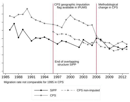
eliminate 1,732 of them because I do not observe any pre-migration earnings and 2,390 that correspond to individuals moving to the State where they were born. To check the representativeness of the SIPP data, in figure 2.1, I display one-year migration rates drawn from SIPP and CPS.12 Interstate migration rates have been decreasing for the last 30 years and this is apparent in both SIPP and CPS. However, the CPS data displays a sharp drop in year 2006 when imputed observations are not disre-garded. Kaplan and Schulhofer-Wohl (2012) investigate the causes of such a drop and conclude that it can be mostly attributed to a methodological change on the missing value imputation procedure. When I drop imputed values, the data displays a much smooth decreasing behaviour, comparable with the one observed in SIPP.13

Figure 2.1: One-year interstate migration rate

CPS geographic imputation flag available in IPUMS

Methodological change in CPS End of overlapping structure SIPP 0 .005 .01 .015 .02 .025 .03 .035 .04

Proportion of interstate moves

1985 1988 1991 1994 1997 2000 2003 2006 2009 2012

SIPP CPS non-imputed CPS

Migration rate not comparable for 1995 in CPS

2.3.1 Migrant Definition

I define as a mover those individuals for whom current state of residence differs from the previous one. The use of States to define alternatives in internal US migration is not new to the literature (e.g. Borjas, Bronars, et al. 1992; Dahl 2002; Kennan and Walker 2011) and it gives me an exhaustive and mutually exclusive division of mainland US that is stable across time. Furthermore, states are typically large enough that local labour markets do not cross state borders and the data shows that is across

12

Construction of moving rates from SIPP require some work. See appendix 2.6.1 for an explana-tion of the procedure.

13

IPUMS provides with an imputation flag from 1995 onwards. Before 1996 imputation rates were marginal (Kaplan and Schulhofer-Wohl 2017).

(31)

2.3. Data 19

states and not at lower levels where labour motives dominate migration events (table 2.10).14 Importantly, the use of States to delimit mobility events makes my results comparable with previous previous work on internal US migration selection (Borjas, Bronars, et al. 1992) and allows for easier replication as different datasets provide publicly available state identifiers but no smaller geographical areas (see Molloy et al. 2011).15

Within those that move across states, there is a marked age profile in terms of mobility motives (figure 2.2). Those movers that are 25-55 years old tend to report moving across states due to new job or job transfer. For older movers the dominant reason is housing reasons, or family reasons if above 60, and for younger movers the dominant motive is family reasons with a clear decreasing profile between age 16 and 25. In the analysis, I take this into account and produce estimates with all 16-65 working individuals and 25-55 only.

That few individuals declare having moved to look for work or due to job lost suggest that a large proportion of those who move due to job related reasons have engaged on non-local job search and, therefore, it is feasible to obtain ex-ante wage information at other locations. This is supporting evidence for a minimal condition for selection in the Borjas model: movers must know the distribution of wages at other locations.

14_{Nonetheless, states may cover multiple labour markets and some interstate migration events} may not involve labour market changes (Kaplan and Schulhofer-Wohl 2017; Molloy et al. 2011).

15_{Other definitions of locations in the US migration literature include Standard Metropolitan} Statistical Area (e.g. Bishop 2012; Gabriel and Schmitz 1995) and distance based measures (Ham et al. 2011).

(32)

Figure 2.2: Moving Reason Age Profile 0.00 0.25 0.50 0.75 1.00 20 30 40 50 60 Age Family reasons New job or job transfer

To look for work or lost job For easier commute

Retired

Other job−related reason

Housing reasons Other reasons

Note: Pooled 1984-2013 CPS data, excluding 1995. In CPS an individual is defined as a migrant if one year ago she was living in a different state, with the exception of year 1995 where the time interval refers to five years prior to the interview (see Faber 2000). Those that move across states

only.

Finally, what is more convoluted to define is the population against which one will compare the characteristics of movers. The usual procedure in the literature (e.g. Borjas, Bronars, et al. 1992; Fernandez-Huertas Moraga 2011; Parey et al. 2017; Spitzer and Zimran 2018) is to take a window of time, often times defined by the sample window, on which if an individual is observed moving she is classified as a migrant and otherwise as a stayer. Although, this is an undeniably interesting exer-cise, it does not quite match the layout of the model. Those that are not observed moving do not represent the population form which migrants are drawn and can be potentially much different if selection is strong. Actually, recovering the distribution of skills in the population can be a daunting challenge when there are many possible destinations, even with a highly parametrized framework as the Borjas model.16 In-stead of trying to recover the population distribution or using the population at risk of migration (as referred by Spitzer and Zimran 2018), I compare skill distributions of movers across destinations. This has the advantage of distributions been directly recoverable from the data and matches perfectly the layout of the model. In section 2.2, I show that the distribution of skills for movers to the least disperse location is dominated by the population while the distribution of those moving to the most disperse location dominates the population. Then, to test the implications of the

16_{Dahl (2002) provides a semi-parametric estimator to recover the population first moments that} he uses to estimate differences in returns to education across US states in a multiple market Roy model.

(33)

2.3. Data 21

model, I can just compare the distribution of skills for those moving to the least dis-perse location with the distribution of those moving to more disdis-perse locations and, if the model gives a sufficiently good description of the selection mechanism, I should observe that selection turns positive as I increase dispersion at destination.

2.3.2 Measuring Skill and Dispersion

I follow Fernandez-Huertas Moraga (2011) and use pre-migration earnings measured at the last observation before migration as my measure of migrant skill. From pre-migration earnings I derive three measures of skill: predicted earnings, pre-pre-migration standardized residuals and the aggregation of the two. To compute predicted earnings and residuals, similarly to Borjas, Bronars, et al. (1992), I use the following wage equation

witj =βxit+γt+ωj+itj (2.12) Where x contains a constant, a quadratic on age and dummies for sex, race, highest education level attained, industry, and occupation. δ and γ are year and state dummies. I control for occupation and industry because individuals specialize within these, as one can observe in tables 2.1 and 2.11 where movers tend to find a job within the same industry or occupation as their last pre-migration job.

Table 2.1: Occupation Transitions of Movers (Row Proportions)

Current Occupation

Previous Occupation Manager High/Medium Skilled Low Skilled Farmer

Manager 0.914 0.069 0.016 0.000

High/Medium Skilled 0.044 0.921 0.033 0.002

Low Skilled 0.028 0.089 0.876 0.007

Farmer 0.050 0.067 0.117 0.767

A possible concern is that the OLS estimates of returns to characteristics from an equation like (2.12) may be biased due to immigrant selection. However, estimators in the literature correcting for migrant selection (Dahl 2002; Parey et al. 2017) return estimates that are close to OLS. Thus I use OLS estimates from specification (2.12) to obtain a measure of predicted,βx, and residual,, pre-migration earnings. In the case of residual earnings, I follow Borjas, Bronars, et al. (1992) and divide them by the earnings variance of the state where the earnings were generated to account for differences in variance that are given by differences in unobservable skill pay-off across locations. Then, using the standardized measure of residual earnings (∗), I construct standardized pre-migration earnings as w∗ = βx+∗, this is my third measure of skill.

(34)

Another concern when using earnings to measure selection is whether they may be modified by or in anticipation of migration (Fernandez-Huertas Moraga 2011; Spitzer and Zimran 2018). Fernandez-Huertas Moraga (2011) and McKenzie et al. (2010) test whether there are earnings drops right before migration, similar to those in the program participation literature (Ashenfelter 1978), without finding any significant changes. In unreported results, I tested whether the difference between the earliest observation of earnings and the last observation before migration are significant. I find non statistically significant differences after controlling for experience and calendar year effects.

To rank locations I follow the model tightly and use earnings dispersion. I pro-duce dispersion estimates using data from IPUMS-CPS because in the CPS all states are individually identified, while in the SIPP some states are grouped together. This implies that only with CPS data I can effectively rank all states according to their earnings dispersion. From the CPS I compute within year and state earnings dis-persion and residual-earnings disdis-persion from a wage equation controlling for sex, ethnicity and education. Whether I choose to use earnings or residual-earnings to measure dispersion does not make much difference in terms of empirical results. This is expected given the strong correlation between the two measures. Nonetheless, what makes a difference is the temporal aggregation. Taking the average of the yearly earn-ings dispersion estimates for each state and regressing raw pre-migration wages on the dispersion ranking produces a strong positive estimate. Moving up one position in the ranking of the destination location correlates with a .4% increase on pre-migration earnings. However, the effect reduces to .1% if I rank locations according to yearly dispersion estimates instead of averages of yearly estimates (table 2.2). Measurement error may explain why I see smaller estimates when I rank location by year dispersion instead by decade or whole sample averages. This is because averaging observations across time may reduce the extend of measurement error and, therefore, the impact of attenuation bias.

The selection effect on wages is robust to controls for sex, ethnic group and age. Although it reduces to .2% when I introduce controls for whether the individual has no education, has completed up to 4th grade, has a high school diploma or is a degree graduate. Additionally, controlling for industry and occupation reduces the selection effect further but only when ranking locations according to yearly dispersion or decade averages.

(35)

2.3. Data 23

Table 2.2: Rank of Destination and Pre-Migration Earnings

(1) (2) (3) (4) (5) (6) Rank (fixed) .004∗∗∗ .004∗∗∗ .004∗∗∗ .004∗∗∗ .002∗∗∗ .002∗∗∗ (.001) (.001) (.001) (.001) (.001) (.001) Rank (decade) .003∗∗∗ .003∗∗∗ .003∗∗∗ .003∗∗∗ .002∗∗∗ .001∗∗ (.001) (.001) (.001) (.001) (.001) (.001) Rank (year) .001∗ .001∗∗ .001∗∗ .001∗∗ .0001 −.0001 (.001) (.001) (.001) (.001) (.001) (.001) Observations 9,217 9,217 9,217 9,217 9,217 9,217 Controls Sex N Y Y Y Y Y Ethnicity N N Y Y Y Y Age N N N Y Y Y Education N N N N Y Y Industry N N N N N Y Occupation N N N N N Y

Note: Each estimate in the table comes from an independent regression. Clustered standard errors by previous state in paranthesis. All columns include fixed effects for state of origin and year. Characteristics and earnings measured at last observation before migration. p< .1 .

, p< .05 *, p< .01 **, p< .001 ***

Changes in the magnitude of selection effects estimates from column (4) to (5) in table 2.2 suggest that selection on observables might be stronger in terms of education, with mild or no selection in terms of sex, age and ethnicity. That is exactly what I observe when looking at those characteristics across location groups delimited by earnings dispersion (table 2.12). Individuals with a degree are over-represented among those moving to the most disperse group of locations (G5) as compared with those moving to the least disperse location group (G1, the baseline in table 2.12). The same is true for those in managerial occupations moving into the most disperse group of locations. In terms of sex and ethnicity I do not find statistically significant selection. Throughout my analysis of stochastic dominance in section 2.4 I aggregate loca-tions into groups according to earnings dispersion. I do this because otherwise sample sizes become too narrow as to be able to draw any meaningful inference. In particu-lar, I aggregate locations into groups using earnings dispersion according to table 2.3. Reducing the number of possible destinations from 51 to 5 gives me sufficient sample size to test the implications of the model in terms of stochastic dominance.

(36)

Table 2.3: Dispersion groups

Group Definition

G1 if dispersion is below 20th percentile G2 if dispersion between 20th-40th percentile G3 if dispersion between 40th-60th percentile G4 if dispersion between 60th-80th percentile G5 if dispersion above 80th _percentile

Within dispersion groups as defined in table 2.3, locations are not clustered ge-ographical or in terms of average earnings (figure 2.3). In the most disperse group (G5) there are states from the west coast (California), south (New Mexico, Texas and Louisiana), the east coast (Virginia, New Jersey, New York, Connecticut and Massachusetts) and northern states (Michigan). Some of these states, those in the east coast, are also at the top in terms of average earnings, while others, the south, are at the bottom. This within group variation in terms of geographical location and average earnings helps on making sure that the selection patterns observed in the data are not driven by state characteristics other than earnings dispersion.

Figure 2.3: Ranking of Locations

(a)Dispersion Groups

G1 G2 G3 G4 G5

(b) Average Earnings

E1 E2 E3 E4 E5

Before going into testing stochastic dominance relations, I test whether the selec-tion patter that emerged in terms of average earnings in table 2.2 is still present when I aggregate locations into groups. In table 2.13, I regress pre-migration earnings on a set of dummies for each of the dispersion groups. As when using rankings, I observe that as the dispersion of the destination location increases average earnings mono-tonically increase. Also, as in table 2.2, introducing controls for education reduces the extend of selection and this gets further reduced when I control for occupation and industry. Thus the selection profile implied by the model is still there in terms of average earnings when testing it across earnings dispersion groups.

Finally, an implication from the theory that gets overseen is that earnings dis-persion of the location where skills are measured, in this case the previous location,

(37)

2.4. Stochastic Dominance 25

do not play a role in determining the direction of selection, but it does affect the intensity of selection. Higher dispersion at the previous location creates a stronger degree of selection, see (2.8). In table 2.4, I regress pre-migration earnings on the rank of the destination conditioning on dispersion of the home location. What I ob-serve is precisely the pattern implied by the theory. Positive selection increases as the earnings dispersion increases and the magnitude of the selection effect increases with dispersion of the previous location. For example, for those that were in a location in the least disperse group (G1), a one position increase in the ranking of the destination location increases wages by .1%. The same increase in the ranking of the destination location produces a selection effect of .5% for those moving from a location in the most disperse group (G5).

Table 2.4: Selection Interacted with Location Group of Origin

Home Location Dispersion Group

G1 G2 G3 G4 G5

Rank .001 .002 .003∗ .004∗∗∗ .005∗∗∗ (.002) (.002) (.002) (.001) (.001) Observations 639 1,394 1,606 2,257 3,321

Note: Each estimate in the table comes from an independent regression. Clustered standard errors by previous state in paranthesis. All columns include fixed effects for year. Characteristics and earnings measured at last observation before migration. p< .1._{, p}_{< .}_{05 *, p}_{< .}_{01 **, p}_{< .}_{001 ***}

2.4 Stochastic Dominance

To provide a formal test of the model implications I use Davidson and Duclos (2013) restricted stochastic dominance test. Davidson and Duclos (2013) test departs from most of the previous literature on testing for stochastic dominance as it posts a null of non-dominance. Aside from its simplicity, testing a null of non-dominance effectively ranks the distributions under study. However, for continuous distributions the null of non-dominance can never be rejected at the tails of the distribution. This leads to a test of restricted stochastic dominance over an interval [z−, z+]. In my application, I set z− to be the 5% quantile and z+ the 99% and test whether I can reject the null of non-dominance when comparing the distribution of pre-migration earnings of migrants moving to the least disperse location group against each other location group. This is

F(z|j∈G1)≤F(z|j∈Gk) (2.13) against the alternative hypothesis

(38)

F(z|j∈G1)> F(z|j∈Gk)

at various z in the interval [z−, z+] for each location group (k) other than the least disperse one. In what follows, I present figures comparing the distribution of skill measures of those moving to the least disperse group and all other groups, jointly with bootstrap p-values for Davidson and Duclos (2013) restricted dominance test.

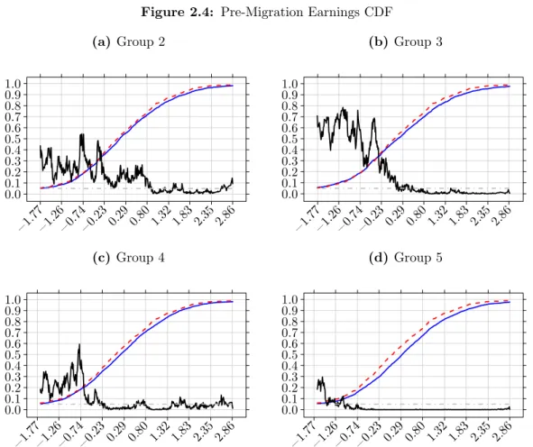
In figure 2.4, I present evidence of selection in terms of pre-migration standardized earnings. In all sub-figures, I present the distribution of pre-migration standardized earnings for those moving into the least disperse location in a dashed red line and the distribution of those moving into the location group that I am comparing in solid blue. Jointly with these two distributions, I provide bootstrap p-values for the point-by-point null in (2.13) constructed with 500 replication samples for each point. The bootstrap samples are drawn using empirical likelihood probabilities constrained under the null as described in Davidson and Duclos (2013).

When I compare the distribution of pre-migration earnings of those moving to the least and second least disperse location (figure 2.4a) the null of non-dominance can only be rejected at small and discontinuous points of the distribution. This means that there is no evidence of dominance between these two distributions. However, as I increase the dispersion of the destination location the dominance relations implied by the model become apparent. The earnings distribution of those moving into the third least disperse location group dominates the distribution of those moving to the least disperse location from the 70% quantile and up. This threshold decreases to around the 20% quantile when looking at those that move into the second most disperse group and close to the 10% quantile when comparing movers to the least disperse group with movers to the most disperse group. The data, therefore, displays the selection pattern predicted by the model: the earnings of those moving to the most disperse location dominates the earnings of those moving to the least disperse and for those locations in the middle there is somehow intermediate selection. As noted by Borjas, Kauppinen, et al. (2018), selection in terms of stochastic dominance provides stronger evidence for the implications of the model than selection in terms of average wages. This is because stochastic dominance implies ordering of the first moments but not the opposite.

(39)

2.4. Stochastic Dominance 27

Figure 2.4: Pre-Migration Earnings CDF

(a)Group 2 0.0 0.1 0.2 0.3 0.4 0.5 0.6 0.7 0.8 0.9 1.0 −1.77−1.26−0.74−0.23 0.29 0.80 1.32 1.83 2.35 2.86 (b) Group 3 0.0 0.1 0.2 0.3 0.4 0.5 0.6 0.7 0.8 0.9 1.0 −1.77−1.26−0.74−0.23 0.29 0.80 1.32 1.83 2.35 2.86 (c) Group 4 0.0 0.1 0.2 0.3 0.4 0.5 0.6 0.7 0.8 0.9 1.0 −1.77−1.26−0.74−0.23 0.29 0.80 1.32 1.83 2.35 2.86 (d) Group 5 0.0 0.1 0.2 0.3 0.4 0.5 0.6 0.7 0.8 0.9 1.0 −1.77−1.26−0.74−0.23 0.29 0.80 1.32 1.83 2.35 2.86

Notes: Red dashed line is the CDF of pre-migration earnings of those moving into the least dis-perse locations. The black line is the point-by-point bootstrap, 500 replications per point, p-value of Davidson and Duclos (2013) stochastic dominance test. Dashed grey line at .05

The same selection pattern on pre-migration earnings is displayed by the data if I select those that are 25-55 years old, figure 2.7. Individuals in this age range, as I show in table 2.2, are the ones most likely to be moving due to labour market motives. Furthermore, selection is driven by both male, figure 2.8, and female, 2.9, movers. For females positive selection at the top of the pre-migration earnings distribution is only found for those moving to the most disperse location group. Females moving to the third least disperse exhibit positive selection but only, roughly, between the 50-90% quantiles and for females moving to the second most disperse group selection happens, roughly, between the 70-90% quantile. For male movers, I observe the same pattern as with the whole population, although p-values are more volatile.

Another possible way on which one could use Davidson and Duclos (2013) re-stricted dominance test, is to search for the longest interval, [z−, z+], on which one can reject the null of non-dominance at a given significance level. This is interesting because it implies that the closer the bonds of the rejection interval are to the bottom and top of the joint support the more power the test has (Davidson and Duclos 2013). When carrying this test the null is over the maximum statistic in the interval [z−, z+]

(40)

max

z∈[z−_,z+_](F(z|G5)−F(z|G1))≥0

In table 2.5, I present p-values for this null for various intervals. Comparing the distribution of earnings of movers to the least (G1) and second least disperse (G2) location groups shows that there is no clear ordering of the two distributions. There is no interval on which the null of non-dominance can be rejected. A similar conclusion is true for comparison of the least disperse group with the third least disperse group (G3). Although, in that case, the null of non-dominance can be rejected to the right of the median. For the most (G5) and second most disperse (G4) groups, the null of non-dominance can be rejected from the median to the 99% quantile. To the left of the median the null of non-dominance can be rejected at the 90% confidence level over the interval [.3, .5] for the second most disperse group and over the interval [.2,.5] for the most disperse group. Thus the nested test confirms what was already found with the point by point test: the distribution of earnings for movers follows the selection pattern implied by the theory.