MSI Working Paper

(1)

MSI_1508

The sensitivity of R&D investments to cash flows:

Comparing young and old EU and US

leading innovators

(2)

1

The sensitivity of R&D investments to cash flows: Comparing young

and old EU and US leading innovators

Michele Cincera (ULB), Julien Ravet (ULB), Reinhilde Veugelers (KULeuven & Bruegel)

This version: 20/4/2015 Abstract

Using firm level information on the world leading R&D investors and employing a system GMM estimation, this paper investigates how sensitive R&D investments are to cash flow movements, which would be suggestive of financial constraints. The analysis confirms that over the last decade the R&D investments of younger aged leading innovators appear to be more sensitive to cash flows compared to their older counterparts and that this holds particularly for EU younger aged leading innovators compared to their US counterparts, particularly in medium and high tech sectors.

Keywords: EU-US R&D gap, younger aged leading innovators, cash-flow sensitivity, R&D investments JEL codes: C23, E22, O31, O33

1. INTRODUCTION

The EU innovation environment remains to date weak, especially R&D investment by the business sector. Furthermore, not much progress can be observed. US companies continue to perform better than their EU counterparts.1

The persistent deficiency of private R&D spending in Europe is a symptom rather than a cause, with the cause rooted in the structure and dynamics of European industry and enterprise. Cincera and Veugelers (2013a) show that the European Union’s business research and development deficit relative to the United States can be almost entirely accounted for by the EU having fewer younger aged firms among its leading innovators (or “yollies”) of the likes of Google, Amazon, Amgen,… and even more importantly having yollies that are less R&D intensive: having fewer yollies accounts for 34% of the EU-US business R&D gap, while having less R&D intensive yollies accounts for 55% of the EU-US business R&D gap. The lower R&D intensity of older aged EU leading innovators accounts for merely 11% of the EU-US business R&D gap.

What explains why Europe has less younger aged leading innovators, but particularly why they invest relatively less in R&D compared to their US counterpart? Cincera and Veugelers (2013b) investigate whether the lower R&D investment rates in the EU can be associated with lower rates of return to R&D. Their econometric analysis indeed finds evidence confirming lower rates of return to R&D investments for European yollies compared to their US counterparts.

Such lower rates of return to R&D may not only impede European yollies to engage in R&D investments. This lower rate of return may also kill the appetite for financiers to fund their projects.

1 _{In 2012, R&D by US private companies represented nearly 2% of the US GDP while business R&D in Europe} only accounted for 1.22% of EU GDP. Source: Eurostat, OECD.

(3)

2

Access to external finance is indeed an important barrier for innovating firms. Cincera and Ravet (2010) analyse the existence and importance of financing constraints for R&D investments for large EU and US manufacturing companies. Using the sensitivity of R&D investments to cash flow variations as a signal of financial constraints, they show a higher sensitivity for European firms compared to their US counterparts. But this analysis does not look at the differences between younger and older innovators. Younger aged innovators, particularly when they have more risky innovative projects, are typically expected to be more affected by financial barriers as compared to older aged innovators (Brown et al., 2009).

This paper investigates in more detail the access to finance issue as a possible cause for the persistent business R&D gap of the EU relative to the US. Building further on the finding that the lower R&D investments of European “yollies” are the major source of this deficit, we want to investigate whether financial constraints might correlate with a lower R&D investment readiness of European “yollies”. Using firm level information on the world leading R&D investors, we examine through econometric analysis whether the R&D investments of younger aged world leading innovators (“yollies”) are more sensitive to cash flow changes, suggestive of facing more financial constraints for funding their R&D projects, compared to older aged world leading innovators (“ollies”), and whether this would hold more for European “yollies” compared to their US counterparts.

The analysis indeed confirms that over the last decade the R&D investments of young leading innovators appear to be more sensitive to cash constraints compared to their older counterparts and that this holds especially for EU young leading innovators, especially in medium and high tech industries. This finding thus correlates with the lower engagement in R&D investments of European “yollies” compared to the US, driving a major part of the EU-US business R&D gap. Before we present the results in section 4, we first present our research methodology to measure financing constraints (section 2) and the data used in the analysis (section 3).

2. METHODOLOGIES TO ASSESS FINANCING CONSTRAINTS

As we are looking for the causes of the R&D deficit of the EU versus the US and the lower R&D investment readiness of young leading innovators in the EU, we are particularly interested in any differences in financing constraints of leading innovators from the US versus the EU, and particularly for younger aged leading innovators. Accessing external finance may be more difficult for younger aged innovators, particularly when they hold more risky projects compared to their mature counterparts. This would imply that younger firms will have to rely more heavily on their internal funds to finance their R&D projects. Mature firms often have sufficient cash-flow for their investment and depend less on equity or debt issues (Brown et al., 2009). Hence, increasing the supply of internal funds should have more impact on the R&D decisions of younger firms compared to more mature firms.

2.1. A review of empirical methodologies to assess financing constraints

A commonly used methodology in the empirical literature to assess financing constraints for investment decisions is the estimation of a standard investment equation where a variable for the availability of internal finance is added to the model (usually cash flow) (Fazzari et al., 1988). Its significance (and correct sign) should signal the relevance of financing constraint in the firm's investment decisions. The idea behind the investment sensitivity to cash flows, is to measure the importance of retained earnings in the R&D investment decision. Hall and Lerner (2010) motivate this

(4)

3

approach as an experiment that consists in giving additional cash to a company, and observing whether they use it for investment or not. If they pass it to shareholders, either there is no good investment opportunity, or the cost of capital has not fallen. If the additional amount of cash is used for investment, it would mean that the firm has unexploited investment opportunities for which external finance is too costly.

This methodological framework has become a standard toolbox for studying financial constrains faced by firms when investing in R&D. It has been used by, among others, Harhoff (1998), Bond et al. (1999), Mairesse, Mulkay and Hall (1999), Mulkay et al. (2001), Brown et al (2012) and more recently Lööf and Nabavi (2014). Most of the studies find internal financing an important determinant of R&D expenditures, suggestive of financial constraints, e.g. Himmelberg and Petersen (1994) for large incumbent US firms, Harhoff (1998) for German firms, Cincera (2003) for Belgian firms, Bond, Harhoff and Van Reenen (2003) for British firms, but not for German firms, which the authors attribute to institutional differences in financial systems in the two countries. Brown et al. (2012) after controlling for smoothing and equity finance access, find financial constraints for R&D investments for a large sample of European firms.

The monotonicity of the relationship between the investment to cash-flow sensitivity and the level of financing constraints in the Fazzari approach has been criticized in the literature, most notably by pointing to the neglect of the possibility of external finance (Kaplan and Zingales, 1997). Moyen (2004) shows that when firms can use debt as a substitute for internal finance, a sensitivity of investment to cash-flow can be generated even when there is no financing friction. This result arises when current debt is correlated with contemporaneous cash-flow. Nevertheless, the conventional interpretation of the investment to cash-flow sensitivity (i.e. a sensitivity that reveals financing constraints) still holds for constrained firms that do not have “sufficient funds to invest as much as desired. Constrained ﬁrms without funds to invest more have investment policies that are more

sensitive to cash flow fluctuations than those of other firms.” Even if firms have access to funds, they

may still be constrained to access sufficient funds for financing their R&D investment projects, particularly when these carry high levels of riskiness.

Furthermore, as also claimed by Kaplan and Zingales (1997), the interpretation of the estimated coefficient associated with the cash flow ratio can be misleading since cash flow can be correlated with current profitability. In this case, cash flow will also be a proxy of profit or demand expectations and the effect of this variable cannot be interpreted unambiguously as evidence of financing constraints. Dealing with this problem requires controlling for profit or demand expectations. Various approaches have been used to better control for this. Himmelberg and Petersen (1994) use changes in output as better proxies for changes in demand than the cash flow variable. This allows them to control, even if imperfectly, for demand expectations. Another avenue is to consider the projections of future profits on past variables and use them as implicit proxies for the expectations of future profits (Abel and Blanchard, 1986). Bond and Meghir (1994) implement a structural Euler equation model derived from the intertemporal maximization problem of the firms. However, as pointed out by Butzen, Fuss and Vermeulen (2001) among others, this last approach, while more appropriate from a theoretical point of view, has often failed to produce significant and correctly signed parameters.

Another major problem with the empirical approach to estimate cash-flow sensitivity of investment decisions, is the presence of other firm characteristics, which may be driving investment decisions and which are correlated with the cash-flow variable, but which may not be observable by the researcher and are therefore not controlled for. The capability of the firm to find new inventions and turn them into successful innovation is one example of such an unobserved firm characteristic. This unobserved capability, linked to the quality of the firm’s R&D personnel or its managerial skills, is likely to be ‘transmitted’ to the R&D decision since firms with higher capabilities or opportunities will invest more in research activities. This in turn will imply a (positive) correlation between these

(5)

4

unobservable variables and the R&D investment which invalidates the inference that can be made from an investment equation estimation.

While econometric techniques such as within and first difference OLS estimators can take care of the biases arising from possible correlated effects, it should be noted that these estimators could still be biased for three other important reasons. The first source of bias can come from random measurement errors in the right hand side variables of the equation. These errors typically tend to be magnified when applying first differences or “within” transformations (Griliches and Hausman, 1986). The two other sources of bias come from (i) the simultaneity between the contemporaneous regressors and the disturbance terms and (ii) the endogeneity of the contemporaneous regressors and the past disturbances. A solution to these three potential sources of bias consists of using an instrumental variable approach by choosing an appropriate set of lagged values of the regressors as instruments. This approach can be implemented by means of a GMM framework such as the one developed by Arellano and Bond (1991) among others. If the original error term follows a white noise process, then values in levels of regressors lagged two or more periods will be admissible instruments.2_{The validity of the instruments is generally verified using the classic Sargan test and}

Hansen test for over-identifying restrictions.3

Arellano and Bover (1995) and Blundell and Bond (1998) developed a system GMM estimator, which combines the instruments of the first difference equation with additional instruments of the untransformed equation in level. Given the higher number of instruments, the system GMM estimator can lead to dramatic improvements in efficiency compared with the first difference GMM estimator.4_{Arellano and Bond (1991), Windmeijer (2005) and Roodman (2006) showed that the}

one-step GMM estimator may be more reliable than the two-one-step one as the latter provide downward biased asymptotic standard errors. However, Windmeijer (2005) developed a small-sample correction for the standard errors of two-step estimators that allows for more accurate inference. While most of the criticisms of the cash-flow sensitivity approach can be addressed by including proper controls and instruments, some studies avoid the problems associated with the cash-flow sensitivity approach by using a direct indicator of financing constraints. This however requires access to data measuring financing constraints directly. Aghion et al. (2012) use a French firm level data set to study the cyclicality of R&D investments and credit constraints. Their direct indicator of credit restrictions is based on non-payments of trade credits. Savignac (2008) looks at the existence and impact of financing constraints using survey data from French firms on their cost of searching, waiting and getting new finance. Czarnitzki and Hottenrott (2011) look at the credit rating scores of innovating firms in Germany.

2.2. Our empirical approach to assess financing constraints

In the absence of direct evidence for financing constraints for our sample of the world largest R&D investing firms, we will look at the sensitivity of their R&D investments to changes in internal funds

2_{As noted by Bond et al. (2003), if the error term in levels is serially uncorrelated, then the error term in the} first difference specification has a moving average structure of order 1 (MA(1)) and only instruments lagged two periods or more will be valid. If the error term in levels already has a moving average structure, then longer lags will have to be considered.

3_{We do not to report the Sargan test statistics. These statistics represent a special case of the Hansen's J} statistics under the assumption of homoscedasticity. Therefore, for robust GMM, the Sargan test statistics are inconsistent (Roodman, 2006).

4_{More fundamentally, as shown by Blundell and Bond (1998), when the autoregressive parameter is high and} the number of time periods is low, the first difference GMM estimator can be subject to a serious finite sample bias as a result of the weak explanatory power of the instruments.

(6)

5

(as measured by cash-flow movements). In this section, we present the investment error-correction equation as well as the econometric methodology we use for estimating the relationship between cash flow movements and R&D investments.

Following a neo-classical approach (Jorgenson, 1963), the logarithm of the desired (or long run) stock of capital is proportional to the logarithm of output and the user cost of capital:

it it t

it

y

c

=

α

+

β

−

σθ

(1)

where c is the logarithm of the stock of R&D, y is the logarithm of the sales and θ is the logarithm of the user cost of capital (UCC). This model can be derived by assuming a profit maximizing firm with a CES production function with elasticity

σ

.

The user cost of capital, as noted by Mulkay et al. (2001), is, in general, difficult to measure at the firm level given the absence of an output price and an investment price at such a disaggregated level. This problem is typically addressed by assuming that the variations in the user cost of capital can be represented by time dummies and specific fixed (long-term) firm effects.5

In order to allow dynamic adjustments of R&D capital, equation 1 is turned into an autoregressive distributed lag model ADL(2,2). This is a standard specification used in the literature. It is convenient for short period samples as it captures temporal dynamics without abusively dropping data in the estimations because of the lag in variables. We obtain the following equation:

1 1 2 2 0 1 1 2 2

it i t it it it it it it

c

=

α α ρ

+

c

₋

+

ρ

c

₋

+

β

y

+

β

y

₋

+

β

y

₋

+

ε

₍₂₎

Following Bond and Meghir (1994), Harhoff (1998) and Mulkay et al. (2001), this equation can be rewritten in an error correction framework:

it it it it it it it t i it

c

y

c

y

c

=

α

+

α

+

λ

∆

+

λ

∆

+

λ

∆

+

λ

−

+

λ

+

ε

∆

0 ₋1 1 2 ₋1 3

(

₋2 ₋2

)

4 ₋2 (3) where

λ

₀

=

ρ

₁

−

1

,

λ =

₁

β

₀,

λ

₂

=

β

₀

+

β

₁,

λ

₃

=

ρ

₁

+

ρ

₂

−

1

and

λ

₄

=

β

₀

+

β

₁

+

β

₂

+

ρ

₁

+

ρ

₂

−

1

.

λ3 is the coefficient of the error correction term and is expected to be negative. λ4, if non-significant,

indicates that returns to scale are constant. By applying the usual approximation6

1

Δ

c

it

≈

R

it

/

C

it−

−

δ

, with R being the R&D expenditures and δ the depreciation rate

of R&D capital, equation 3 becomes:

it it it it it it it it t i it it

y

c

y

C

R

C

R

_α

_λ

_ε

+

−

+

∆

+

∆

+

=

₋ ₋ ₋ ₋ − − − 2 4 2 2 3 1 2 1 2 1 0 1

)

(

(4)

5_{See, however, Butzen, Fuss and Vermeulen (2001) for an application that estimates the user cost of capital.}

6 δ − ≅ ∆ ≅       ₊∆ =       − + =       = − = ∆ − − − − − − − − 1 1 1 1 1 1 1

1) log log log 1

log( ) log( it it it it it it it it it it it it it it it C R C C C C C C C C C C C C c

(7)

6

Following the seminal work of Fazzari et al. (1988) and the many studies using this methodology, we augment equation (4) with cash flow effects (divided by one period lagged C for normalization), which allows to analyze the sensitivity of R&D investments to variations in cash flow available to firms, suggestive of firms being constrained in accessing funds for their R&D projects:

2 4 2 2 3 1 2 1 2 1 0 1

)

(

₋ ₋ ₋ − − − −

+

−

+

∆

+

∆

+

=

_it _it _it _it _it it it t i it it

y

c

y

C

R

C

R

_α

_λ

it it it it it

C

CF

C

CF

_λ

_ε

λ

+

− − − 2 1 6 1 5 (5)

We employ a system GMM framework to deal with biases from unobserved and correlated factors. Estimates are obtained from a two-step procedure, which uses as instruments the level of the regressors lagged two till up to five periods and more, combined with the first lag of their first difference.7_{We use the Windmeijer correction for the reported two-step estimators. The validity of}

different sets of instruments are tested with the Sargan and Hansen over-identification tests. The null hypothesis is that the instruments are valid, i.e. they are uncorrelated with the error terms. Under the null hypothesis, the test statistic follows a chi-squared distribution with a number of degrees of freedom being equal to the number of over-identifying restrictions. Rejection of the null hypothesis casts a doubt on the validity of the set of instruments.

As we are interested in any differences between leading innovators from the US versus the EU, and particularly for younger aged leading innovators, we will look for differential sensitivity to cash flows between these sub-samples of firms. We expect a higher sensitivity for younger aged leading innovators, especially for those based in the EU compared to their US counterparts.

3. DATA

Our empirical analysis is based on a representative sample of the largest US and EU R&D active companies in the manufacturing and services sectors. We used the successive editions of the EU industrial R&D investment scoreboards (2004 – 2008) conducted by the JRC-IPTS of the European Commission. According to JRC-IPTS, these scoreboards are representative of more than 85% of all R&D carried out in the private sector in the world.8_{As such, explaining the R&D investments of these}

firms, being among the largest R&D investors in the world, can go a long way in explaining the EU-US overall R&D deficit, which is why we focus on this sample.

The Scoreboard data are matched with the Compustat database in order to gather financial information, including the cash flow of the firms.9_{The dataset has been merged with the one used by}

Cincera and Veugelers (2013a) to include the age of the firms. The final sample used in the empirical analysis consists of an unbalanced panel of 888 firms over 2000–2007. All variables are presented

7_{Results are robust to different sets and lags of instruments.}

8 _{Background information and methodology of the 2008 R&D Scoreboard:} http://iri.jrc.ec.europa.eu/research/docs/2008/Methodology.pdf.

9_{The cash flow variable used in this study is equal to the income before extraordinary items, which represents} the income of a company after all expenses except provisions for common and or preferred dividends, plus depreciation and amortization, which are the non-cash charges for obsolescence and wear and tear on property.

(8)

7

using constant exchange rates and price indexes. R&D stocks are constructed for each firm on the basis of the perpetual inventory method (Griliches, 1979). For each firm, the R&D stock at time t is defined by: s t s s t t t t t t C R R R R R C ₋ ∞ = − − − + = + − + − + =

∑

− − = 0 2 1 1 (1 ) (1 )² ... (1 ) ) 1 (

δ

(6)

This expression assumes that the current state of knowledge relies on current and past R&D expenditures. Fixing the magnitude of the depreciation rate is not straightforward as it is likely to vary in time and across firms (for instance according to the technology level used). Most literature assumes a depreciation rate of 15%. By testing different values for δ, Hall and Mairesse (1995) find small or no changes in the estimation of the R&D capital effect.10_{Hence we also rely on a classic}

depreciation rate set to 0.15. The initial value of C can be computed by using the following expression11_:

δ

+

=

g

R

C

₀ 0 (7)

where g is the growth rate of R and is assumed to be constant. The growth rate that is used in this study is the sample average12_{growth rate of R&D expenditures in the industry.}13_{According to Hall}

and Mairesse (1995), the choice of g affects directly the initial stock but its importance declines over time.

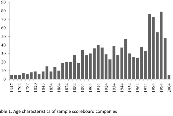
The scoreboard data we use is only representative for the largest R&D investors in the world. It does not cover small firms. When we distinguish innovators on their age profile, the younger aged firms should not be considered as representative of small young start-ups. The younger aged innovators in our sample, denoted as “yollies” (younger aged leading innovators), are younger in age than the more mature world leading innovators, denoted as “ollies”. Examples of “yollies” include Google, Microsoft, Qualcomm, Amazon, Amgen. They are no longer “small” and “young”, as they already passed their start-up stage, having become among the set of largest R&D investors in the world. Figure 1 and Table 1 show evidence on the age distribution of the world leading R&D firms in our sample. While before 1975 there was a continuous stream of world leading innovators being born, an important wave of new leading innovators were born after 1975. This is a wave mostly riding on the opportunities offered by new digital and biotechnology opportunities. It is this wave of world leading innovators that we want to identify in the analysis as yollies compared to the older world leading R&D firms (ollies). We thus define yollies (young leading innovators) as scoreboard firms that were created after 1974 and ollies before 1975, as in Cincera and Veugelers (2013a).

In total about 59% of the sample Scoreboard firms are yollies, a ratio which is lower among EU Scoreboard firms (56%). Most of these yollies can be found in High and Medium Tech sectors, most

10_{See also Griliches and Mairesse (1983, 1984).}

11_{This expression can be derived from the definition of the R&D stock in equation 2.7,}

∑

∞ = − − = 0 ) 1 ( s s t s t R C δ .

The latter equation leads to

∑

∞

= − − = 0 0 0 ) 1 ( ) 1 ( s s R g C δ and thus 2.8.

12_{The average growth rate for an industry is computed as the average of the distribution of individual growth} rates inside the range [Q1 – 1.5(Q3-Q1), Q3 + 1.5(Q3-Q1)] where Q1 and Q3 are the first and third quartiles of the distribution.

(9)

8

notably in ICT and biotech.14_{US firms have a higher share of their}_yollies_{present in high-tech sectors}

compared to the EU (66% vs 46%) (see also Cincera and Veugelers, 2013a).

The analysis does not change much when taking more recent years for distinguishing yolllies versus

ollies. Taking more recent years leaves lower number of observations in the yollies categories. For

instance, using 1990 as the cutoff rate for defining yollies leaves 400 yollies (compared to 522 using 1975) 15

Insert Table 1 and Figure 1 here

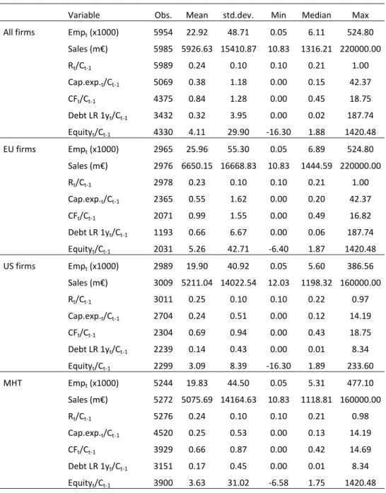
Table 2 reports some descriptive statistics. It shows the big size of the firms in our sample: the median leading innovator employs 6100 employees. Yollies are smaller but nevertheless still big: the median yollie employs more than 3000 people. Table 2 also shows descriptive statistics on the cash flow and R&D investment positions of the sample firms. It shows that yollies have on average a lower relative cash flow position compared to ollies, but they have a higher R&D investment ratio. Table 2 also shows that the smaller sample of yollies using the 1990 cutoff is similar in characteristics than the larger sample of yollies using the 1975 cutoff, used in the analysis.

When comparing the EU versus the US, Table 2 shows that EU scoreboard firms have lower R&D investments, while holding higher cash flow positions than their US counterparts. This holds for all EU firms, but a fortiori for yollies: European yollies have higher cash positions and lower R&D positions relative to their US counterparts. Compared to debt, equity appears to be an important financing source for all sample firms.

Insert Table 2 here

These descriptive statistics are consistent with expectations of higher sensitivity of R&D investments to cash flow positions for yollies, particularly European ones, which would be evidence supporting that these firms face higher financial constraints. The next section will investigate whether econometric analysis can confirm these expectations.

4. ECONOMETRIC RESULTS

4.1.Yollies versus Ollies: All sectors and countries

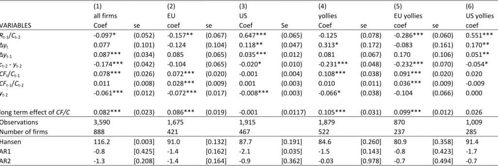
Table 3 shows the system GMM estimates of the R&D error correction model estimated for all sample firms, yollies, EU and US firms and EU and US yollies.16

Insert Table 3 here

14_{High-, medium- and low-tech sectors for ICB industries are defined as in Ortega-Argiles et al. (2009) and} Cincera and Ravet (2014).

15_{Results using the 1990 cutoff rate are not reported for sake of space but can be obtained from the authors} on request.

(10)

9

The Hansen test validates the set of instruments used except for column (1), which is the column for all observations pooled. The second order correlation test statistics do not suggest any problems with the time structure of the sets of instruments. With the exception of columns 2 and 6, the error correction term has the expected negative sign and is statistically significant at the 1 % level. The coefficient of output lagged by two periods is negative (except in column 6) and significant albeit only slightly. This suggests the presence of slightly decreasing returns to scale. The positive and significant coefficients associated with the changes in output (except for cols 2 and 5) suggest positive expectations of future profitability to the extent that these variables are a proxy of the investment opportunities of a firm.17

Our major variables of interest are the Cash Flow variables. They have in general a positive and significant effect on R&D investment, supporting that the R&D investments of world leading innovators are sensitive to cash flow fluctuations, suggestive that world leading innovators are constrained in obtaining sufficient funds for their R&D projects. When we compare EU and US firms, the results confirm Cincera and Ravet (2010), namely that only EU leading innovators’ R&D investments are sensitive to cash flow movements, while no significant effect is found for their US counterparts (cols 2 and 3 in Table 3). Our findings are different from other studies who find that US firms appear more financially constrained (Hall et al., 1999; Mulkay et al. 2001; Bond et al. 1999).A first difference between Mulkay et al. (2001) and our paper is that in the former only France and US are compared while we compare the US with all EU28 countries. Our set of EU countries includes the UK whose companies’ R&D investments are found to be more sensitive to cash flow than their continental German counterparts (Bond, Harhoff and Van Reenen, 1999). Second, our period of analysis is not the same. We analyse the decade 2000-2010 while the period studied in Mulkay et al. is the 90’s. The world's financial systems have undergone fundamental changes since 2000 affecting the EU and the US differently (Cincera and Ravet, 2010).

When we compare the sensitivity of R&D investments to cash flow movements depending on the age profile of scoreboard firms, we find that these effects are significantly more important for yollies (col 1 and 4 in Table 3). A one unit increase of the contemporaneous cash-flow variable yields an increase of the R&D investment accumulation rate of .11 for yollies against .078 for all firms. The results therefore confirm that the R&D investments of yollies are more sensitive to cash flow movements. Looking only at EU yollies (col 5), seriously reduces the number of observations. Nevertheless, the results show that the R&D investments of EU yollies are indeed significantly sensitive to cash flow movements, while this does not hold for their US counterparts. The long-term coefficient associated with the cash-flow variables is about .099 for EU yollies against .03 for US yollies.

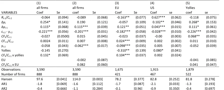
Rather than splitting the samples by age and region, which reduces sample size, and since we are mostly interested in differences in the cash flow coefficients only, we perform the same system GMM analysis but with interaction effects with age or region dummies on the cash flow variables.18

These are reported in Table 4.

Insert table 4 here

17_{We also estimated fixed effects models (with and without interaction terms). The results are robust to the} ones obtained with GMM.

18_{One advantage of this type of specifications is that the sample of firms is held constant across models. Hence} the differences in the estimated rates of returns to R&D are not due to differences in the samples’ composition.

(11)

10

The interaction effect results confirm that yollies are more sensitive to cash flow fluctuations for their R&D investment decisions as compared to ollies (col 1), that EU leading innovators are more sensitive compared to US leading innovators (col 2), and that EU yollies are more sensitive compared to EU ollies (col 3). For US firms there does not seem to be any significant difference in cash flow sensitivity between young and old leading innovators (col 4). Column 5 shows that EU yollies’ R&D investments are more sensitive to cash flows fluctuations than US yollies, but the difference is not significant.

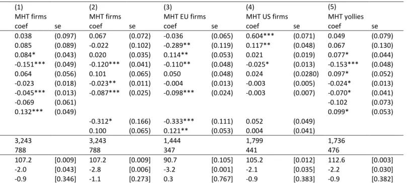
4.2.Yollies versus Ollies: High and Medium Tech

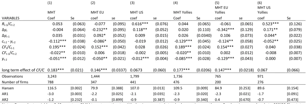
As a further robustness check, we perform the analysis on the sample of scoreboard firms from the Medium and High Tech (MHT) sectors only.19_{These results are reported in Table 5 and Table 6.}

Insert Tables 5 and 6 here

The analysis finds first that the R&D investment of scoreboard firms in MHT sectors are more sensitive to cash flow movements than their counterparts in Low Tech sectors. This MHT effect follows from comparing cols (1) in Table 3 and Table 5.

In line with the results found for the total sample, the results also confirm that the R&D investments of EU leading innovators in MHT are more cash flow sensitive than their US counterparts (comparing cols 2 and 3 in Table 5 and col 1 in Table 6).

The results on yollies in the MHT subsample (col 4 in Table 5) confirm that, like in the total sample,

MHT yollies are sensitive to cash flow fluctuations for their R&D decisions, suggestive of being

financially constrained. The size of the coefficient does not seem to be very different from all firms. In the European MHT subsample, yollies display a higher sensitivity than ollies, while there is no significant difference between ollies and yollies in the US MHT subsample. So, unlike their US counterparts, the R&D investments of EU MHT yollies seem significantly more sensitive to cash flow movements than EU MHT ollies. Col (5) in Table 6 shows that while the R&D investments of EU yollies

in MHT sectors are significantly sensitive to cash flow movements, this does not hold for the US

yollies in these sectors.

To sum up, the R&D sensitivity to cash-flow appears to be higher for yollies, in particular for EU

yollies which indicates that these companies rely more on their cash-flow in order to finance their

R&D investments. US yollies seem to have no different cash flow sensitivity from US ollies. These results hold for medium and high tech sectors in particular. Hence our results are consistent with the view that EU yollies do less R&D particularly in medium- and high-tech sectors being exposed to more severe financing constraints for their R&D investments.

5. CONCLUSIONS

In an attempt to understand better the persistent EU business R&D deficiency relative to the US, more particularly why Europe has less R&D investments coming from younger aged leading

19_{Including only the High-Tech sectors would seriously reduce the number of firms in the analysis, particularly} European yollies.

(12)

11

innovators, we use a representative sample of the largest worldwide private companies active in R&D, to investigate the sensitivity of their R&D investments to cash flow movements. Measuring the sensitivity of R&D investments to cash flow fluctuations is a commonly used approach in the literature to assess whether firms are constrained in accessing sufficient funds for their R&D projects. We estimate a cash flow augmented error correction equation for R&D investments. We use a system GMM estimator with the Windmeijer correction.

Our results confirm that the R&D investments of EU leading innovators are more sensitive to cash flow movements than their US counterparts, particularly in medium- and high-tech sectors. When differentiating according to the age of the leading innovators, we find that the R&D investments of younger aged leading innovators (“yollies”) are significantly more sensitive to the availability of internal finance, compared to their older aged counterparts, which suggests they are facing more financing constraints on R&D. This holds particularly in medium- and high-tech sectors. This higher sensitivity of young firms holds only for EU yollies. US yollies seem to face no significantly different cash sensitivity compared to US ollies. Particularly in medium- and high-tech sectors, EU yollies are significantly more sensitive to cash flow movements for their R&D investments than US yollies. Higher cash flow sensitivity of R&D investments, suggestive of financial constraints, may thus clarify the lower presence and the lower R&D investment intensity of young leading innovators in the European R&D landscape as compared to the US, in particular in the high-tech sectors.

Although it is clear that the often more risky projects of young leading innovators, particularly in high tech sectors, should at least not be disadvantaged in public funding programs over those from incumbent leading innovators, our analysis at this stage cannot yet be used to motivate targeting “yollies” by public funding agencies. This requires also a comparison with the financial constraints faced by other potential targets such as young, small innovators. In order to further investigate this question, a larger sample would be needed which would include, besides large younger aged R&D investors, also small young R&D investors.

Beyond expanding the sample to include more smaller and younger innovators, further robustness checks need to confirm the results before sound policy conclusions can be drawn. Particularly the use of other empirical methodologies to assess financial constraints than the currently used cash-flow sensitivity approach would be helpful. But this requires other sources of information on financial constraints, which are not readily available.

If further analysis confirms the financial constraints of younger aged innovators in Europe, the next question to address is what causes the discrepancy in financing of firm R&D investments between European and US markets.

(13)

12

REFERENCES

Abel A.B. and O.J. Blanchard. 1986. "The Present Value of Profits and the Cyclical Movements in Investment." Econometrica 54: 249-273.

Aghion P., P. Askenazy, N. Berman, G. Cette and L. Eymard. 2012. "Credit constraints and the cyclicality of R&D investment: Evidence from France." Journal of the European Economic Association 10(5): 1001-1024.

Aghion P., E. Bartelsman, E. Perotti and S. Scarpetta. 2008. "Barriers to exit, experimentation and comparative advantage." RICAFE 2 WP 056, London School of Economics.

Arellano M. and S. Bond. 1991. "Some Tests of Specification for Panel Data: Monte Carlo Evidence and Application to Employment Equations." Review of Economic Studies 58: 277-97.

Arellano M. and S. Bond. 1998. "Dynamic Panel Data Estimation Using DPD98 for Gauss: A guide for Users", mimeo.

Blundell R. and S. Bond. 1998. "Initial Conditions and Moment Restrictions in Dynamic Panel Data."

Journal of Econometrics 87: 115-143.

Bond S., J. Elston, J. Mairesse and B. Mulkay. 2003. "Financial Factors and Investment in Belgium, France, Germany and the U.K.: A Comparison Using Company Panel Data." Review of Economics and

Statistics 85: 153–165.

Bond S., D. Harhoff and J. Van Reenen. 1999. "Investment, R&D and Financial Constraints in Britain and Germany." Institute for Fiscal Studies Working Paper #W99/05.

Bond S. and C. Meghir. 1994. "Dynamic Investment Models and the Firm’s Financial Policy." Review

of Economic Studies 61(2): 197-222.

Brown J.R., S.M. Fazzari and B.C. Petersen. 2009. "Financing innovation and growth: Cash flow, external equity, and the 1990s R&D boom." Journal of Finance 64(1): 151-185.

Brown J.R. and B.C. Petersen. 2009. "Why has the investment-cash flow Sensitivity declined so sharply? Rising R&D and equity market developments." Journal of Banking and Finance 33: 971-984. Brown, J. R., Martinsson, G. and B.C. Petersen. 2012. "Do financing constraints matter for R&D?"

European Economic Review 56(8): 1512–1529

Butzen P., C. Fuss and P. Vermeulen. 2001. "The Interest Rate and Credit Channels in Belgium: An Investigation with Micro-Level Firm Data." National Bank of Belgium, Working Papers Research Series, 18.

Cincera M. 2003. "Financing constraints, fixed capital and R&D investment decisions of Belgian firms." in P. Butzen, and C. Fuss, Firms’ Investment and Finance Decisions: Theory and Empirical Methodology, Cheltenham, UK: Edwar Elgar, 129-147.

Cincera M. and R. Veugelers. 2013a. "Young Leading Innovators and the EU’s R&D intensity gap."

Economics of Innovation and New Technology 22(2): 177-198.

Cincera M. and R. Veugelers 2013b. "Exploring Europe’s R&D deficit relative to the US: Differences in the rates of return to R&D of young leading R&D firms." iCite WP 2013-1, Université Libre de Bruxelles.

Cincera M. and J. Ravet. 2010. "Financing constraints and R&D investments of large corporations in Europe and the USA." Science and Public Policy 37(6): 455-466.

Cincera M. and J. Ravet. 2014. "Globalisation, Industrial Diversification and Productivity Growth in Large European R&D Companies." Journal of Productivity Analysis 41(2): 227- 246.

(14)

13

Cohen E. and J.-H. Lorenzi. 2000. "Politiques industrielles pour l’Europe." Conseil d'Analyse Economique Rapport 26, La Documentation française.

Czarnitzki, D. and H. Hottenrott. 2011. "R&D investment and financing constraints of small and medium-sized firms." Small Business Economics 36(1): 65-83.

European Commission. 2007. "Key figures 2007 on Science, Technology and Innovation Towards a European Knowledge Area." ISBN 9279034502.

European Commission. 2008. "Analysis of the 2007 EU Industrial R&D Investment Scoreboard." Joint Research Centre - Institute for Prospective Technological Studies and Directorate General Research, Scientific and Technical Report series, JRC45683, EUR 23442 EN, ISBN 978-92-79-09562-7, ISSN 1018-5593, see: http://ftp.jrc.es/EURdoc/JRC45683.pdf.

Fazzari S.M., R.G. Hubbard and B.C. Petersen. 1988. "Financing Constraints and Corporate Investment." Brookings Papers on Economic Activity 1: 141-195.

Fazzari S.M., R.G. Hubbard and B.C. Petersen. 2000. "Investment-Cash Flow Sensitivities Are Useful: A Comment on Kaplan and Zingales." Quarterly Journal of Economics 115(2): 695-705.

Griliches Z. 1979. "Issues in assessing the contribution of research and development to productivity growth." The Bell Journal of Economics 10(1): 92-116.

Griliches Z. and J.A. Hausman. 1986. "Errors in Variables in Panel Data." Journal of Econometrics, 31, 93-118.

Griliches Z. and J. Mairesse. 1983. "Comparing Productivity Growth: An Exploration of French and US Industrial and Firm Data." European Economic Review 21: 89-119.

Griliches Z. and J. Mairesse. 1984. "Productivity and R&D at the Firm Level." in Z. Griliches (ed.), “R&D, Patents and Productivity”, University of Chicago Press, Chicago, 339-374.

Hall B.H. and J.Lerner. 2010. "Financing R&D and Innovation." in B.H. Hall and N. Rosenberg (eds.), "Handbook of the Economics of Innovation", Elsevier Handbook of the Economics of Innovation, 609-639.

Hall B.H. and J.Mairesse. 1995. "Exploring the Relationship Between R&D and Productivity in French Manufacturing Firms." Journal of Econometrics 65: 263-94.

Harhoff D. 1998. "Are There Financing Constraints for R&D and Investment in German Manufacturing Firms?" Annales d'Economie et de Statistiques 49-50: 421-56.

Himmelberg C.P. and B.C. Petersen. 1994. "R&D and Internal Finance: A Panel Study of Small Firms in High-Tech Industries" Review of Economics and Statistics 76(1): 38-51.

Jorgenson D.W. 1963. "Capital Theory and Investment Behaviour." American Economic Review 53(2): 247-259.

Kaplan S.N. and L. Zingales. 1997. "Do Investment-Cash Flow Sensitivities Provide Useful Measures of Financing Constraints." Quarterly Journal of Economics 112(1): 169-215.

Kaplan S.N. and L. Zingales. 2000. "Investment-Cash Flow Sensitivities are Not Valid Measures of Financing Constraints." Quarterly Journal of Economics 115(2): 707-712.

Mairesse J., B. Mulkay and B.H. Hall. 1999. "Firm-Level Investment in France and the United States: An Exploration of What we Have Learned in Twenty Years." National Bureau of Economic Research Working Paper 7437.

Moncada-Paterno-Castello P., C. Ciupagea, K. Smith, A. Tübke and M. Tubbs. 2010. "Does Europe perform too little corporate R&D? A comparison of EU and non-EU corporate R&D performance."

(15)

14

Mulkay B., B.H. Hall and J. Mairesse. 2001. "Investment and R&D in France and the United States." in Herrmann Heinz and Rolf Strauch (eds.), “Investing Today for the World of Tomorrow”, Springer Verlag.

O’Mahony M. and B. van Ark. 2003. "EU Productivity and Competitiveness: An industry Perspective - Can Europe Resume the Catching-up Process?" Office for Official Publications of the European Communities. Luxembourg. ISBN 92-894-6303-1.

Ortega-Arguiles M., L. Potters and M. Vivarelli. 2009. "R&D and Productivity: Testing Sectoral Peculiarities Using Micro", IPTS Working Paper on Corporate R&D and Innovation, No.03/2009. Luxembourg: Office.

O’Sullivan M. 2007. "The EU's R&D deficit and innovation policy." Report of the Expert Group on ‘Knowledge for Growth’, European Commission DG Research.O’Mahoney and van Ark, 2003

Roodman D. 2006. "How to do Xtabond2: An Introduction to Difference and System GMM in Stata." Center for Global Development, Working Paper 103.

Savignac F. 2008. "Impact of Financial Constraints on Innovation: What Can Be Learned from a Direct Measure?" Economics of Innovation and New Technology 17(6): 553-69.

Windmeijer F. 2005. "A finite sample correction for the variance of linear efficient two-step GMM estimators." Journal of Econometrics 126: 25–51.

(16)

15

Figure 1. Distribution of firms in the sample by year of foundation

Table 1: Age characteristics of sample scoreboard companies # of scoreboard firms Mean Age of Scoreboard firms

# of Yollies Mean Age

of Yollies Share of Yollies in High-Tech

EU 421 99 237 18 46

US 467 55 285 20 66

(17)

16

Table 2: Descriptive statistics

Variable Obs. Mean std.dev. Min Median Max

All firms Empt (x1000) 5954 22.92 48.71 0.05 6.11 524.80

Sales (m€) 5985 5926.63 15410.87 10.83 1316.21 220000.00 Rt/Ct-1 5989 0.24 0.10 0.10 0.21 1.00 Cap.exp.t/Ct-1 5069 0.38 1.18 0.00 0.15 42.37 CFt/Ct-1 4375 0.84 1.28 0.00 0.45 18.75 Debt LR 1yt/Ct-1 3432 0.32 3.95 0.00 0.02 187.74 Equityt/Ct-1 4330 4.11 29.90 -16.30 1.88 1420.48 EU firms Empt (x1000) 2965 25.96 55.30 0.05 6.89 524.80 Sales (m€) 2976 6650.15 16668.83 10.83 1444.59 220000.00 Rt/Ct-1 2978 0.23 0.10 0.10 0.21 1.00 Cap.exp.t/Ct-1 2365 0.55 1.62 0.00 0.20 42.37 CFt/Ct-1 2071 0.99 1.55 0.00 0.49 16.82 Debt LR 1yt/Ct-1 1193 0.66 6.67 0.00 0.06 187.74 Equityt/Ct-1 2031 5.26 42.71 -6.40 1.87 1420.48 US firms Empt (x1000) 2989 19.90 40.92 0.05 5.60 386.56 Sales (m€) 3009 5211.04 14022.54 12.03 1198.32 160000.00 Rt/Ct-1 3011 0.25 0.10 0.10 0.22 0.97 Cap.exp.t/Ct-1 2704 0.24 0.51 0.00 0.12 14.19 CFt/Ct-1 2304 0.69 0.94 0.00 0.43 18.75 Debt LR 1yt/Ct-1 2239 0.14 0.43 0.00 0.01 8.34 Equityt/Ct-1 2299 3.09 8.39 -16.30 1.89 233.60 MHT Empt (x1000) 5244 19.83 44.50 0.05 5.31 477.10 Sales (m€) 5272 5075.69 14164.63 10.83 1118.81 160000.00 Rt/Ct-1 5276 0.24 0.10 0.10 0.21 0.98 Cap.exp.t/Ct-1 4520 0.25 0.53 0.00 0.13 14.19 CFt/Ct-1 3929 0.66 0.87 0.00 0.42 14.69 Debt LR 1yt/Ct-1 3151 0.17 0.45 0.00 0.01 8.34 Equityt/Ct-1 3900 3.63 31.02 -6.58 1.75 1420.48

(18)

17

Table 2 (continued)

Variable Obs. Mean std.dev. Min Median Max

Founded ≥ 1975 Empt (x1000) 3634 9.60 24.89 0.05 3.03 386.46 (yollies) Sales (m€) 3661 2603.97 10042.90 10.83 651.67 220000.00 Rt/Ct-1 3665 0.25 0.11 0.10 0.22 1.00 Cap.exp.t/Ct-1 3036 0.38 1.42 0.00 0.11 42.37 CFt/Ct-1 2315 0.72 1.18 0.00 0.38 18.75 Debt LR 1yt/Ct-1 1833 0.15 0.56 0.00 0.00 8.34 Equityt/Ct-1 2280 3.58 17.83 -6.40 1.79 690.59 EU found. ≥ 1975 Empt (x1000) 1788 11.14 31.12 0.05 3.37 386.46 Sales (m€) 1798 3132.70 13005.33 10.83 699.72 220000.00 Rt/Ct-1 1800 0.23 0.11 0.10 0.21 1.00 Cap.exp.t/Ct-1 1360 0.58 1.99 0.00 0.17 42.37 CFt/Ct-1 1088 0.87 1.32 0.00 0.45 14.69 Debt LR 1yt/Ct-1 655 0.25 0.72 0.00 0.04 8.01 Equityt/Ct-1 1058 4.00 23.31 -6.40 1.79 690.59 US found. ≥ 1975 Empt (x1000) 1846 8.11 16.65 0.05 2.72 232.00 Sales (m€) 1863 2093.70 5872.68 12.03 603.73 120000.00 Rt/Ct-1 1865 0.26 0.11 0.10 0.23 0.97 Cap.exp.t/Ct-1 1676 0.21 0.59 0.00 0.08 14.19 CFt/Ct-1 1227 0.58 1.03 0.00 0.33 18.75 Debt LR 1yt/Ct-1 1178 0.09 0.43 0.00 0.00 8.34 Equityt/Ct-1 1222 3.22 11.06 -5.56 1.80 233.60 Founded ≥ 1990 Empt (x1000) 2955 10.16 26.92 0.05 2.92 386.46 Sales (m€) 2981 2636.62 10737.97 10.83 611.31 220000.00 Rt/Ct-1 2985 0.24 0.11 0.10 0.21 1.00 Cap.exp.t/Ct-1 2433 0.44 1.57 0.00 0.13 42.37 CFt/Ct-1 1705 0.83 1.29 0.00 0.43 18.75 Debt LR 1yt/Ct-1 1291 0.18 0.65 0.00 0.01 8.34 Equityt/Ct-1 1670 4.00 19.49 -6.40 1.98 690.59 EU found. ≥ 1990 Empt (x1000) 1672 11.49 32.06 0.07 3.37 386.46 Sales (m€) 1681 3225.18 13355.79 10.83 694.73 220000.00 Rt/Ct-1 1683 0.23 0.10 0.10 0.20 1.00 Cap.exp.t/Ct-1 1268 0.61 2.06 0.00 0.18 42.37 CFt/Ct-1 987 0.89 1.29 0.00 0.46 13.15 Debt LR 1yt/Ct-1 589 0.27 0.76 0.00 0.04 8.01 Equityt/Ct-1 957 3.86 22.57 -6.40 1.86 690.59 US found. ≥ 1990 Empt (x1000) 1283 8.42 18.02 0.05 2.27 232.00 Sales (m€) 1300 1875.56 5726.46 12.03 510.60 120000.00 Rt/Ct-1 1302 0.26 0.12 0.10 0.23 0.97 Cap.exp.t/Ct-1 1165 0.26 0.70 0.00 0.09 14.19 CFt/Ct-1 718 0.74 1.29 0.00 0.40 18.75 Debt LR 1yt/Ct-1 702 0.11 0.53 0.00 0.00 8.34 Equityt/Ct-1 713 4.20 14.35 -5.56 2.22 233.60

Note: Emp = employees, R = R&D investment, CF = cash flow, C = stock of R&D, Debt LR 1y = long run debt due in one year, Equity = ordinary equity, Cap. Exp. = capital expenditure, MHT = Medium/High-tech.

(19)

18

Table 3: Yollies split sample results: all sectors

(1) (2) (3) (4) (5) (6)

all firms EU US yollies EU yollies US yollies

VARIABLES Coef se coef se Coef Se Coef se coef se coef se

Rt-1/Ct-2 -0.097* (0.052) -0.157** (0.067) 0.647*** (0.065) -0.125 (0.078) -0.286*** (0.060) 0.551*** (0.138) ∆yt 0.077 (0.101) -0.124 (0.104) 0.118** (0.047) 0.313* (0.172) -0.083 (0.161) 0.170** (0.081) ∆yt-1 0.087*** (0.034) 0.085 (0.065) 0.035*** (0.012) 0.081 (0.067) 0.170 (0.106) 0.051** (0.024) ct-2 - yt-2 -0.174*** (0.042) -0.104 (0.065) -0.020* (0.010) -0.231*** (0.048) -0.232*** (0.070) -0.054* (0.033) CFt/Ct-1 0.078*** (0.026) 0.072*** (0.020) -0.001 (0.004) 0.108*** (0.038) 0.091*** (0.020) 0.020 (0.023) CFt-1/Ct-2 0.011 (0.008) 0.028*** (0.009) 0.001 (0.003) 0.010 (0.011) 0.036*** (0.009) -0.009 (0.008) yt-2 -0.061*** (0.012) -0.072*** (0.017) -0.008*** (0.003) -0.066* (0.038) -0.104 (0.066) 0.000 (0.007) long term effect of CF/C 0.082*** (0.023) 0.086*** (0.019) -0.001 (0.0117) 0.105*** (0.031) 0.099*** (0.012) 0.026 (0.040)

Observations 3,590 1,675 1,915 1,879 870 1,009

Number of firms 888 421 467 522 237 285

Hansen 116.2 [0.003] 91.0 [0.132] 87.7 [0.191] 84.6 [0.260] 80.9 [0.358] 91.4 [0.126]

AR1 -0.8 [0.425] -1.4 [0.162] -2.1 [0.035] -1.5 [0.143] -0.8 [0.423] -1.7 [0.093]

AR2 -1.3 [0.208] -1.4 [0.164] -0.9 [0.362] -0.03 [0.978] -0.7 [0.494] -0.7 [0.464]

Notes: Dependent variable = Rt/Ct-1; system GMM two step estimates; Windmejer corrected standard errors in parentheses; P-values in square brackets; ***(**,*) = stat. significant at the 1% (5%, 10% level); instruments = observations dated t-2 to t-4 for Xt (transformed equation) and t-1 for ΔXt (equation in level); all regressions include time and industry dummies.

(20)

19

Table 4: Yollies interaction effect results: all sectors

(1) (2) (3) (4) (5)

all firms all firms EU US Yollies

VARIABLES Coef Se coef Se Coef Se Coef se coef se

Rt-1/Ct-2 -0.064 (0.094) -0.089 (0.068) -0.163** (0.077) 0.627*** (0.062) -0.118 (0.075) ∆yt 0.254* (0.141) 0.190 (0.121) -0.057 (0.109) 0.102** (0.046) 0.268* (0.153) ∆yt-1 0.115* (0.068) 0.115*** (0.039) 0.121** (0.051) 0.043*** (0.015) 0.111* (0.061) ct-2 - yt-2 -0.221*** (0.056) -0.201*** (0.031) -0.182*** (0.058) -0.028*** (0.010) -0.226*** (0.042) CFt/Ct-1 -0.027 (0.0500) 0.015 (0.045) -0.023 (0.037) -0.00 (0.003) 0.068** (0.035) CFt-1/Ct-2 0.0024 (0.011) 0.007 (0.008) 0.024*** (0.009) 0.002 (0.002) 0.011 (0.010) yt-2 -0.058 (0.043) -0.062*** (0.017) -0.098*** (0.035) 0.005 (0.007) -0.052 (0.039) Yollies -0.145 (0.270) -0.310** (0.139) 0.080* (0.041) CFt/Ct-1 x yollies 0.132* (0.069) 0.104*** (0.037) 0.002 (0.024) EU -0.002 (0.087) -0.041 (0.085) CFt/Ct-1 x EU 0.082 (0.060) 0.041 (0.047) Observations 3,590 3,590 1,675 1,915 1,879 Number of firms 888 888 421 467 522 Hansen 97.6 [0.041] 114.0 [0.003] 78.2 [0.377] 82.8 [0.252] 81.8 [0.278] AR1 -1.8 [0.069] -1.6 [0.112] -1.7 [0.087] -2.1 [0.033] -1.3 [0.193] AR2 -0.4 [0.666] -1.1 [0.284] -0.1 [0.96] -0.9 [0.350] -0.4 [0.697]

(21)

20

Table 5: Yollies split sample medium/high-tech (MHT) results

(1) (2) (3) (4) (5) (6)

MHT MHT EU MHT US MHT Yollies MHT EU Yollies MHT US Yollies

VARIABLES Coef Se coef se coef se Coef Se coef se coef Se

Rt-1/Ct-2 0.053 (0.063) -0.077 (0.095) 0.616*** (0.076) 0.044 (0.065) -0.061 (0.065) 0.523*** (0.126) ∆yt -0.004 (0.064) -0.232** (0.095) 0.118** (0.052) 0.020 (0.110) -0.342*** (0.129) 0.171** (0.079) ∆yt-1 0.035 (0.031) 0.092* (0.052) 0.009 (0.015) 0.026 (0.0340) 0.106 (0.073) 0.044* (0.022) ct-2 - yt-2 -0.112*** (0.038) -0.086* (0.050) -0.019 (0.012) -0.129*** (0.045) -0.124** (0.058) -0.052** (0.025) CFt/Ct-1 0.195*** (0.024) 0.152*** (0.042) 0.028 (0.026) 0.189*** (0.024) 0.154*** (0.027) 0.040 (0.038) CFt-1/Ct-2 -0.022** (0.010) 0.006 (0.018) -0.002 (0.005) -0.020** (0.010) 0.002 (0.012) -0.008 (0.007) yt-2 -0.051*** (0.012) -0.050** (0.021) -0.012*** (0.004) -0.085*** (0.028) -0.129*** (0.043) 0.000 (0.007) long term effect of CF/C 0.183*** (0.021) 0.146*** (0.0337) 0.0673 (0.060) 0.177*** (0.0206) 0.147*** (0.0218) 0.067 (0.066)

Observations 3,243 1,444 1,799 1,736 765 971

Number of firms 788 347 441 476 200 276

Hansen 116.5 [0.002] 79.9 [0.388] 107.0 [0.013] 109.5 [0.009] 84.9 [0.253] 89.6 [0.154]

AR1 -3.0 [0.003] -2.2 [0.025] -2.1 [0.035] -2.3 [0.020] -2.3 [0.021] -1.7 [0.091]

AR2 -1.2 [0.232] -0.1 [0.899] -0.9 [0.387] -0.9 [0.340] 0.4 [0.670] -0.7 [0.473]

(22)

21

Table 6: Yollies MHT interaction effect results

(1) (2) (3) (4) (5)

MHT firms MHT firms MHT EU firms MHT US firms MHT yollies

VARIABLES coef se coef se coef se coef se coef se

Rt-1/Ct-2 0.038 (0.097) 0.067 (0.072) -0.036 (0.065) 0.604*** (0.071) 0.049 (0.079) ∆yt 0.085 (0.089) -0.022 (0.102) -0.289** (0.119) 0.117** (0.048) 0.067 (0.130) ∆yt-1 0.084* (0.043) 0.020 (0.035) 0.114** (0.053) 0.021 (0.019) 0.077* (0.044) ct-2 - yt-2 -0.151*** (0.049) -0.120*** (0.041) -0.110** (0.048) -0.025* (0.013) -0.153*** (0.048) CFt/Ct-1 0.064 (0.056) 0.101 (0.065) 0.050 (0.048) 0.024 (0.0280) 0.097* (0.052) CFt-1/Ct-2 -0.023 (0.018) -0.023** (0.011) -0.004 (0.013) -0.003 (0.005) -0.024* (0.013) yt-2 -0.045*** (0.013) -0.087*** (0.025) -0.098*** (0.024) -0.003 (0.007) -0.070* (0.041) EU -0.069 (0.061) -0.102 (0.073) CFt/Ct-1 x EU 0.132*** (0.049) 0.099* (0.053) Yollies -0.312* (0.166) -0.333*** (0.111) 0.052 (0.049) CFt/Ct-1 x yollies 0.100 (0.065) 0.121** (0.053) 0.004 (0.041) Observations 3,243 3,243 1,444 1,799 1,736 Number of firms 788 788 347 441 476 Hansen 107.2 [0.009] 107.2 [0.009] 90.7 [0.105] 105.2 [0.012] 112.6 [0.003] AR1 -2.0 [0.043] -2.8 [0.006] -3.2 [0.001] -2.1 [0.035] -2.2 [0.030] AR2 -0.9 [0.346] -1.1 [0.273] 0.3 [0.767] -0.9 [0.383] -0.9 [0.382]

(23)

22

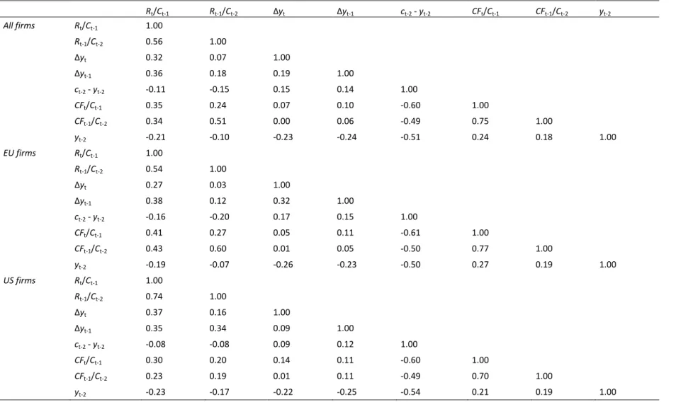
Table 7: Correlation matrix

Rt/Ct-1 Rt-1/Ct-2 ∆yt ∆yt-1 ct-2 - yt-2 CFt/Ct-1 CFt-1/Ct-2 yt-2 All firms Rt/Ct-1 1.00 Rt-1/Ct-2 0.56 1.00 ∆yt 0.32 0.07 1.00 ∆yt-1 0.36 0.18 0.19 1.00 ct-2 - yt-2 -0.11 -0.15 0.15 0.14 1.00 CFt/Ct-1 0.35 0.24 0.07 0.10 -0.60 1.00 CFt-1/Ct-2 0.34 0.51 0.00 0.06 -0.49 0.75 1.00 yt-2 -0.21 -0.10 -0.23 -0.24 -0.51 0.24 0.18 1.00 EU firms Rt/Ct-1 1.00 Rt-1/Ct-2 0.54 1.00 ∆yt 0.27 0.03 1.00 ∆yt-1 0.38 0.12 0.32 1.00 ct-2 - yt-2 -0.16 -0.20 0.17 0.15 1.00 CFt/Ct-1 0.41 0.27 0.05 0.11 -0.61 1.00 CFt-1/Ct-2 0.43 0.60 0.01 0.05 -0.50 0.77 1.00 yt-2 -0.19 -0.07 -0.26 -0.23 -0.50 0.27 0.19 1.00 US firms Rt/Ct-1 1.00 Rt-1/Ct-2 0.74 1.00 ∆yt 0.37 0.16 1.00 ∆yt-1 0.35 0.34 0.09 1.00 ct-2 - yt-2 -0.08 -0.08 0.09 0.12 1.00 CFt/Ct-1 0.30 0.20 0.14 0.11 -0.60 1.00 CFt-1/Ct-2 0.23 0.19 0.01 0.11 -0.49 0.70 1.00 yt-2 -0.23 -0.17 -0.22 -0.25 -0.54 0.21 0.19 1.00

(24)

FACULTY OF ECONOMICS AND BUSINESS DEPARTMENT OF MANAGERIAL ECONOMICS, STRATEGY AND INNOVATION Naamsestraat 69 bus 3500 3000 LEUVEN, BELGIË tel. + 32 16 32 67 00 fax + 32 16 32 67 32 [email protected] www.econ.kuleuven.be/MSI