Research Article A Comparison of Flame Spread Characteristics over Solids in Concurrent Flow Using Two Different Pyrolysis Models

(1)

Volume 2011, Article ID 250391,9pages doi:10.1155/2011/250391

Research Article

A Comparison of Flame Spread Characteristics over Solids in

Concurrent Flow Using Two Different Pyrolysis Models

Ya-Ting Tseng and James S. T’ien

Department of Mechanical and Aerospace Engineering, Case Western Reserve University, 10900 Euclid Avenue, 418 Glennan Building, Cleveland, OH 44106, USA

Correspondence should be addressed to Ya-Ting Tseng,[email protected] Received 30 October 2010; Accepted 24 February 2011

Academic Editor: Kalyan Annamalai

Copyright © 2011 Y.-T. Tseng and J. S. T’ien. This is an open access article distributed under the Creative Commons Attribution License, which permits unrestricted use, distribution, and reproduction in any medium, provided the original work is properly cited.

Two solid pyrolysis models are employed in a concurrent-flow flame spread model to compare the flame structure and spreading characteristics. The first is a zeroth-order surface pyrolysis, and the second is a first-order in-depth pyrolysis. Comparisons are made for samples when the spread rate reaches a steady value and the flame reaches a constant length. The computed results show (1) the mass burning rate distributions at the solid surface are qualitatively diﬀerent near the flame (pyrolysis base region), (2) the first-order pyrolysis model shows that the propagating flame leaves unburnt solid fuel, and (3) the flame length and spread rate dependence on sample thickness are diﬀerent for the two cases.

1. Introduction

In modeling flame spread over solids, a description of the solid pyrolysis processes is required to complete the coupling between the gaseous flame phase and the solid phase. Typ-ically, a pyrolysis description provides the relationship be-tween the solid mass burning rate and the local conditions of the solid fuel being heated. The detailed chemical steps of the pyrolysis reactions, however, can be very complex, depending on the types of solids, the temperature, the heating rate, the duration, among other things. They may also vary depending on whether the surrounding atmosphere is with or without oxygen. There is an abundance of literature on the pyrolysis of materials. For example, in biomass production, a review

can be found for the pyrolysis of wood and biomass [1].

Polymer pyrolysis and measurement can be found in [2]. A

recent pyrolysis model intended for fire research was oﬀered

in [3].

In model computation of flame spread over solids, sim-plified pyrolysis reactions are needed to make the model

more tractable. For example, Di Blasi [4] has employed a

three-step reaction scheme: solid to vapor, solid to tar, and solid to char. A still simpler scheme is a one-step description to represent the overall solid pyrolysis conversion from solid

to vapor. For cellulose, Kung [5] proposed a first-order

re-action whose rate depends on the first power of the local solid density and the Arrhenius expression on temperature. This has been adopted in many opposed-flow flame spread

works (e.g., [6, 7]). Because of the linear dependence on

local density in the rate expression, the solid fuel is not entirely consumed in a finite length of time or in a finite distance by a spreading flame when using the first-order pyrolysis reaction model. Since some solids are observed to

burn out completely in experiments, Ferkul and T’ien [8],

in their concurrent flame spread model, adopted a zeroth-order pyrolysis reaction which has previously been used in solid propellant studies. The zeroth-order reaction has since

been used in many subsequent works (e.g., [9,10]).

Despite their simplicities, there are fundamental diﬀ

er-ences between the zeroth-order and the first-order pyrolysis models. The pyrolyzing mass burning rate depends only on the surface temperature in the zeroth-order model and is therefore a surface model. In the first-order model, on the other hand, pyrolysis rate depends on the local temperature and density in the interior of the solid so it is an in-depth model. Although both models have been employed in many previous flame spread computations, there is no investigation

(2)

on the diﬀerences they produce on flame spreading charac-teristics. This work will compare the performance of both pyrolysis expressions (zeroth- and first-order) using a de-tailed flame spread model over solids in a low-speed forced concurrent flow. The comparisons include flame and solid profiles, solid mass burning rate distributions, and spread rate as a function of sample thickness.

2. Theoretical Formulation

2.1. Flow and Fuel Configuration. The fuel and flow

config-uration considered in the mathematical model is shown in

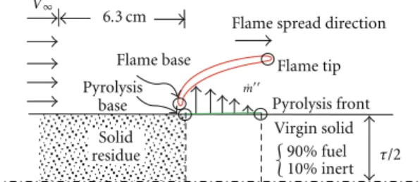
Figure 1. A spreading flame is shown schematically over a

solid sample. The spread is in a two-dimensional concurrent forced flow from left to right (gravity is zero). The flame is on both sides of the sample. Because of symmetry, only one half of the flame is shown and computed. The solid of

thicknessτ consists of one phase of combustible (90%) and

another phase of an inert matrix (10%), so that its structural integrity is retained. As the flame spreads to the right, solid residue is left behind. A uniform laminar forced air flow of

magnitudeV∞is imposed at a distance 6.3 cm upstream of

the flame base. The choice of imposing the upstream flow at a fixed distance is to eliminate the variable entrance length

eﬀect since we are only interested in steady spread in this

work. Experimentally it is also possible to realize a constant entrance length in spreading flames by using a special setup

as demonstrated in [11]. In a previous paper, we have shown

that the flame radiation feedback to the solid can reach up

to 5 cm upstream [12], so the entrance length is chosen to

be greater than this value. Although values other than 6.3 cm can be used, it will not alter the basic physics of the present problem.

2.2. Model Description. With the exception of the pyrolysis

relation, the flame spread formulation is the same as a

previous model [13]. Consequently, we will only mention

briefly the model details except the portion on the formu-lation of the pyrolysis reaction which will be dealt with more thoroughly.

Reference [13] is a transient two-dimensional model

for laminar flame spread over solids in a low-speed forced concurrent flow with zero gravity. It uses an unsteady solid phase and a quasisteady gas-phase. The solid phase consists of an unsteady heat conduction equation with a zeroth-order surface pyrolysis reaction according to the Arrhenius form. The quasisteady gas-phase employs full elliptic Navier-Stokes mass and momentum equations together with energy and species equations. The species considered are fuel vapor,

oxygen, CO2, and H2O. A one-step, second-order

over-all Arrhenius gas-phase reaction is adopted. Both surface and flame radiation are included. The gas-phase radiation transfer equation is solved using the S-N discrete ordinates method so that the radiation flux vectors are determined. More information on the formulation of the gas-phase

processes can be found in [14].

Computations in [13] start with the ignition process.

Flames grow in size initially but eventually reach steady

τ/2

Flame base _{Flame tip}

Pyrolysis

base Pyrolysis front

Solid residue

Virgin solid Flame spread direction

6.3 cm V∞ 90% fuel 10% inert  ˙ m

Figure 1: Configuration of a spreading flame in the computational

model.

states. For a thick solid, the steady state is a nongrowing stationary flame with a limiting length. For a thin solid, the steady state is a spreading flame with a constant spread rate and a constant flame length. The reason for a nongrowing limiting flame for the thick solid is the balance between the flame heat feedback and the surface radiative heat loss at the pyrolysis front. The reason for achieving a steady spread for thin solids is the balance between the solid burnout rate and the flame tip advancing rate. For relatively thin samples, steady spread can be obtained quickly. For thick samples,

the transient growth period may dominate. Reference [15]

shows that the transient pyrolysis process may aﬀect the

flame spread rate quantitatively.

In this work, we will only be interested in thin solids in the steady spreading regime. The steady regime is obtained using the transient program. Please note that, by thin solids, we refer to cases in which the upstream solid fuel burnout (or the spread of the upstream flame base) occurs within the simulation time so that the flame steady spreading state can be achieved. The thermally thin solid assumption is not imposed in this work.

2.2.1. Solid-Phase and Pyrolysis Models

(a) Zeroth-Order (Surface) Pyrolysis. For the zeroth-order

pyrolysis model, the solid heat conduction equation is:

∂ ∂t ρsCsTs = ∂ ∂x ks∂Ts ∂x + ∂ ∂y ks∂Ts ∂y . (1)

It is assumed that the solid pyrolysis occurs only on the

surface and the solid fuel density ρs,F remains constant

during the combustion process. However, as the solid fuel

is depleted, the fuel thickness τF decreases and hence the

composition of the solid changes and the compound solid

density ρs decreases. Until the solid fuel is completely

consumed, the solid becomes pure inert (this will not happen theoretically for the first-order relation). Note also, the

x-y coordinates system in (1) is fixed with respect to the

laboratory. When a steady spread is achieved with a constant

spread velocity Vf, (1) can be transformed into a steady

form with a coordinate transformationx=Vft. So∂/∂t =

(3)

At the interface of the solid-phase and the gas-phase, the energy conservation boundary condition is:

˙

q_c_,in−q˙_r_,out−m˙L=ks

∂Ts

∂y. (2)

In this equation, the convective heat gain, ˙q_c_,in, is obtained

from the quasisteady gas-phase solution, ˙q_r_,out, is equal to

solid surface radiation heat loss minus the flame radiation

feedback, and ˙mLis the energy consumed in pyrolyzing the

solid fuel. Note that both the left- and right-hand sides of (2)

represent the net heat flux entering the interior of the solid, and thus relates to the heat-up of the solid fuel. To facilitate

our discussion, we use ˙qnet,in(=q˙c,in−q˙r,out−m˙L) to denote

this quantity.

To relate the mass burning rate to the surface tempera-ture, a zeroth-order pyrolysis relation is assumed at the fuel surface: ˙ m=Asexp −Es RuTs,w . (3)

This equation indicates that the solid burning rate is very sensitive to the surface temperature for a reasonable value of

Es/Ru(i.e.,1).

(b) First-Order (In-Depth) Pyrolysis. For the first-order

in-depth pyrolysis model, the governing equation for the solid temperature has a more complex expression:

∂ ∂t ρsCsTs + ∂ ∂y( ˙m _C sTs) = ∂ ∂x ks ∂Ts ∂x + ∂ ∂y ks ∂Ts ∂y +L∂ρs,F ∂t . (4)

In this equation, the local fuel vapor mass flux ˙m, resulting

from in-depth pyrolysis, is related to the solid fuel density decrease rate by the mass equation:

∂ρs,F

∂t +

∂m˙

∂y =0. (5)

And with the first-order pyrolysis assumption, we have the following relation: ∂ρs,F ∂t = −AIρs,Fexp ₋ EI RuTs . (6)

In this case, the local solid fuel density decreases during the

burning process. The decreasing rate ofρs,Fis a function of

itself and the local solid temperatureTs. According to (6),

bothρs,Fand ∂ρs,F/∂tnever reach zero as mentioned in the

introduction.

An energy balance is imposed on the surface as the boundary condition:

˙

q_c_,in−q˙_r_,out=ks∂Ts

∂y. (7)

Compared with (2), the latent heat loss term, ˙mL, is not

included. It is because the solid pyrolysis is a “volumetric

phenomenon” instead of a “surface phenomenon.” Hence, the latent heat loss is accounted for in the energy equation

(4), not in the boundary condition. The net heat flux going

into the interior of the solid in this case is ˙q_net,in=q˙_c_,in−q˙_r_,out.

The mass burning rate ˙m on the solid surface is one

of the most important input quantities from the solid phase to the gas-phase. The fuel vapors generated beneath the surface of the solid have to transport to the surface. Here an essential approximation is made, that is, the mass transfer resistance is negligible in the direction perpendicular to the surface because of the small thickness of the solid samples. Consequently, the pyrolyzed fuel vapor inside the solid will reach the surface instantaneously and only in the direction perpendicular to the surface. This is clearly an approximation. For thicker solids, the mass transfer equation

in porous media needs to be solved [16, 17]. With this

assumption, (5) is integrated to obtain the mass burning rate

on the solid surface for the first-order pyrolysis model: ˙

m= τ/2

0 −

∂ρs,F

∂t dy. (8)

Equation (8) states that the mass burning rate (or the fuel

vapor mass flux) on each side of the solid surface is the integration of the density change rate across the half solid

fuel thicknessτ/2.

In the computations, the solid combustible properties other than density are assumed constant. They are based

on cellulose. The solid combustible density ρs,F, remains

constant in the zeroth-order pyrolysis model and varies during the combustion process in the first-order pyrolysis model. The solid combustible thermal conductivity is taken

from [18] (for wood fir in the cross-grain direction). The

inert matrix properties are set to be the same as those of the solid combustible for simplicity (except its density). The inert matrix density is 10% of the virgin solid density. The

solid fuel properties (except AI and EI) can be found in

[13]. The kinetics parameters for the first-order pyrolysis are

AI=1×10101/sec, andEI=3×104cal/mole. They are in the

range of values that are quoted for thin paper samples [19].

2.3. Numerical Scheme. As mentioned earlier, steady

spread-ing solutions are obtained by marchspread-ing in time usspread-ing a

tran-sient numerical code. In a laboratory-fixed x-ycoordinate

system, ignition occurs nearx ≈ 0. The flame base moves

downstream when there is not enough fuel vapor to support the flame locally. Since the flow entrance length is fixed as discussed previously, true steady spread can be obtained. The flame structure and comparisons will be presented when the

flame base is located at anx-location after the steady spread

is achieved. Details of the transient processes can be found in

[13].

One note on the grid size may be worthwhile. A nonu-niform grid structure is adopted in this model. To resolve the flame structure in the stabilization zone (located at the flame base), the chosen characteristic length used to non-dimensionalize the gas-phase equations is the

thermal-dif-fusional distance in the flame stabilization zone,αg/V∞. This

(4)

x(cm) τF / τF,o 20 22 24 26 28 30 32 34 36 38 0.2 0.4 0.6 0.8 1 1E−05 1_E−04 5E−04 y (cm) 0 1 2 3 ωF (a) x(cm) 20 22 24 26 28 30 32 34 36 38 1E−05 1E−04 5E−04 y (cm) 1 2 3 ωF 0 ρs,F/ρs,F0 0.2 0.4 0.6 0.8 0.9 _0.99 ys (cm) −0.03 −0.02 −0.01 0.1 ˙ m₌0.001 g/cm2_/s (b)

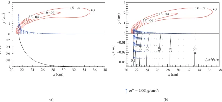
Figure 2: Flame structure, burning rate distribution, and the percentage of un-burnt solid at the steady state (a) with the zeroth-order

pyrolysis model and (b) with the first-order pyrolysis model. Upper plane: contours ofωF(g/cm3s) and ˙mdistribution on the solid surface. Lower plane: (a)τF/τF,0 (b) contours ofρs,F/ρs,F0, and fuel vapor mass flux in the solid. Flow condition:XO2,∞=21%,V∞=5 cm/s, and

ρs,F0τ=28.4 mg/cm2.

αg/V∞ = 0.426 cm for V∞ = 5 cm/s in this work. Finer

grids (0.2 nondimensionalized grid size) are specified in the region close to the flame where the temperature and species gradients are large. Fine grids are also needed in the region

where the flame will pass by. In the solid phase, the x

-direction grids are the same as in the gas-phase. In the y

-direction, uniform grids are specified. Twenty grids in y

-direction are typically used. The detailed grid arrangement

can be found in [13].

3. Computed Results and Discussion

Flame and solid profiles at steady spread conditions are presented and compared first. The leftover un-burnt solid fuel phenomena will be examined next. Lastly, the spread rate variations with sample thickness will be compared between

the two diﬀerent pyrolysis models.

3.1. Flame Structure and Solid Profiles at Steady State. In

order to illustrate the diﬀerences of the flame structure

between zeroth-order and first-order pyrolysis, the steady

state cases with initial area densityρs,F0τ = 28 mg/cm2are

studied (except during the investigation of thickness eﬀect).

We deliberately choose this area density since the flames using both pyrolysis expressions have similar length and

spread rate (lf =8.55 cm,Vf =0.090 cm/s for zeroth-order

pyrolysis andlf =8.83 cm,Vf =0.086 cm/s for first-order

pyrolysis). This facilitates the comparison of the flame and solid profiles.

3.1.1. Mass Burning Rate Distributions. The ˙mdistribution

on the solid surface is the most crucial diﬀerence between

the zeroth-order and first-order pyrolysis models. As shown

on the upper plane of Figure 2(a), for the zeroth-order

pyrolysis, ˙m increases monotonically from downstream

toward the flame base. It reaches the maximum value at the

burnout point (whereτF/τF,0 = 0) and drops oﬀabruptly

to zero upstream. This is implied by (3) in which ˙m is

only a function ofTs,w.Ts,w over the pyrolysis region has a

maximum value at the flame base where the flame standoﬀ

distance is the smallest. As the flame standoﬀ distance

increases,Ts,wdecreases downstream and ˙mdecreases with

Ts,w. Please note that the percentage of un-burnt solid for the

surface pyrolysis case is indicated byτF/τF,0which is shown

on the lower plane inFigure 2(a).

The fuel vapor mass flux ˙m for the first-order

pyrol-ysis case is shown as blue arrows on the lower plane in

Figure 2(b). As mentioned earlier, the fuel vapor produced

in-depth is assumed to convect vertically to the surface with-out mass transfer resistance because of the small thickness of the solid sample. The fuel vapor emerging at the solid-gas interface is the accumulation of the mass flux in-depth

in the solid according to (8). Note that the resulting ˙mon

the solid surface shown on the upper plane ofFigure 2(b)is

very diﬀerent from that of the zeroth-order pyrolysis model.

There is no abrupt cutoﬀand the maximum value occurs

downstream of the pyrolysis base. Instead, ˙m reaches a

maximum (much smaller than that in the zeroth-order case) and then decreases toward zero. This is because in the first-order pyrolysis model, the local burning rate is not only function of local temperature but also local solid fuel density.

AlthoughTsis higher near the pyrolysis base, the lowerρs,F

results in a smaller burning rate. Theρs,F/ρs,F0contours are

also shown on the lower plane ofFigure 2(b)for reference.

(5)

x(cm) ˙ m (g/cm 2/s) 20 22 24 26 28 30 32 0_E+00 5E−04 1_E−03 1.5E−03 2E−03 2.5E−03 3E−03 First-order pyrolysis Zeroth-order pyrolysis x(cm) ˙ m (g/cm 2/s) 20 21 22 100 10−5 10−10 10−15 10−20 10−25 10−30

Figure 3: Fuel vapor mass flux, ˙m distributions on the solid

surface for both pyrolysis models. In the inset, a log-scale ordinate is use d.

surface for the first-order pyrolysis model results in some interesting phenomena which will be discussed later.

The diﬀerent distributions of the surface ˙m between

the two pyrolysis models just discussed are highlighted in

the comparison inFigure 3. The total burning rate, ˙m(the

integration of ˙m over the solid surface) of both cases are

very close (1.35×10−3_{g/cm/s for surface pyrolysis and 1}_.₂₂_×

10−3g/cm/s for in-depth pyrolysis). This is expected since

these two cases have the same area density and similar spread

rates (one can refer to (9) which will be presented later).

Although ˙mfor the first-order pyrolysis case has a smaller

value near the pyrolysis base region (where the un-burnt solid percentage is smaller), it trails longer downstream and has a larger value than that in the zeroth-order pyrolysis

model after x > 23.5 cm. Also, ˙m will not reach zero

inside the flame zone according to our discussion in the introduction. A log-scale ordinate is used to demonstrate this phenomenon in the inset.

3.1.2. Flame Structures. In order to illustrate the flame

structures, gas-phase reaction rateωFand flame temperature

contours are shown on the upper plane of Figures 2 and

4, respectively. Although the flame lengths (defined here by

ωF = 10−4g/cm3s) of these two models are very close,

the flame structures are very diﬀerent. The contours of

ωF in Figure 2indicate that the reaction is more vigorous

near the flame base region for the zeroth-order pyrolysis

case. If one compares the contours ofωF at a higher value,

say 5 × 10−4g/cm3_{s, one would notice that the}

zeroth-order pyrolysis case has a longer flame length (3.0 cm versus

2.3 cm). Also, the maximum value of ωF for the

zeroth-order pyrolysis model is a bit higher than that of the

first-order pyrolysis model (ωF,max = 1.6 ×10−3g/cm3s and

1.5×10−3g/cm3_{s for each model, resp.). However, if one}

compares contours ofωFat a smaller value, say 10−5g/cm3s,

the first-order pyrolysis model has the longer contour length

(14.4 cm versus 15.6 cm). This is the results of the diﬀerent

˙

mdistributions between the two models. Using the

zeroth-order pyrolysis model, ˙m is concentrated near the flame

1.5 1.6 1.7 1.8 1.9 2 2.1 2.5 2.5 1.5 x(cm) ys (cm) 20 22 24 26 28 30 32 34 36 38 −0_.03 −0.02 −0.01 3 4.5 4 5 y (cm) 0 1 2 3 Tnon Tnon s (a) 1.5 1.6 1.7 1.8 1.9 2 2.4 1.5 x(cm) ys (cm) 20 22 24 26 28 30 32 34 36 38 −0.03 −0.02 −0.01 3 4.5 4 5 y (cm) 0 1 2 3 Tnon Tnon s (b)

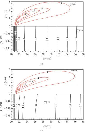
Figure 4: Temperature profiles of the gaseous flame and the

solid phase at the steady state (a) with the zeroth-order pyrolysis model and (b) with the first-order pyrolysis model. Upper plane: nondimensional gas-phase temperature contours. Lower plane: nondimensional solid-phase temperature contours. Temperature is nondimensionalized by 300 K. Ordinate scales are diﬀerent in y

(gas-phase) andys(solid phase).

base region and has a larger maximum value. On the other

hand, ˙mfor the first-order pyrolysis case is more distributed

along the solid surface.

The temperature contours in Figure 4further illustrate

the flame structures of both cases. Similarly, if one compares contours of the nondimensional value 4, both models give a similar contour length. But one would find the zeroth-order pyrolysis model has a longer contour length by comparing contours of a larger value and a shorter contour length by comparing contours of a smaller value.

3.1.3. Heat Fluxes on the Solid Surface. As discussed earlier,

these two pyrolysis models have a diﬀerent energy balance on

the solid surface (refer to (2) and (7)). Heat flux distributions

on the solid surface for both models are shown inFigure 5.

In this figure, the convective heat flux, ˙qc,in (red line) and

(6)

x(cm) 20 22 24 26 28 30 32 34 36 38 ˙_q (cal/cm 2/s) −0.1 0 0.1 0.2 0.3 0.4 0.5 0.6 0.7 ˙ m_L ˙ q c,in ˙ q

r,out q˙net, in=q˙c,in−q˙r,out−m˙L

(a) x(cm) 20 22 24 26 28 30 32 34 36 38 ˙ q (cal/cm 2/s) −0_.1 0 0.1 0.2 0.3 0.4 0.5 0.6 0.7 ˙ q c,in ˙ q_r,out ˙ q

net, in=q˙c,in−q˙r,out

(b)

Figure 5: Heat fluxes on solid surface at the steady state (a) with the zeroth-order pyrolysis model and (b) with the first-order pyrolysis

model. y (cm) 0 1 2 0.01 0.02 0.03 0.05 0.06 0.1 0.5 0.8 0.9 0.99 x(cm) ys (cm) 12 14 16 18 20 22 24 26 28 −0.03 −0.02 −0.01 (a) 0.03 0.05 0.07 0.08 0.09 0.095 0.098 Y (cm) 0 1 2 0.1 0.5 0.8 0.9 _0.99 x(cm) ys (cm) 10 12 14 16 18 20 22 24 26 −0.03 −0.02 −0.01 (b)

Figure 6: Solid leftover occurs when flames are near the extinction limit. (a)XO2,∞=16% (b)XO2,∞=15%. Upper plane: indication of

visible flame shape. Lower plane: solid residual fuel percentage. (contours ofρs,F/ρs,F0). Ordinate scales are diﬀerent iny(gas-phase) andys (solid phase).

have the same features for both models. However, the net

heat fluxes going into the interior of the solid, ˙q_net,in(orange

line), are very diﬀerent. For the zeroth-order case, ˙q_net,in

is very close to zero over the entire pyrolysis region as

shown in Figure 5(a). It is because surface pyrolysis takes

place and consumes the energy from the flame. Please note

that ˙q_net,in has a small finite value around the pyrolysis

front which preheats the solid fuel and enables the flame to spread downstream. This phenomenon is discussed in a

previous paper [13]. The solid temperature profile is shown

inFigure 4(a). It is shown that the solid fuel is thermally thin

in this case.

In comparison, the heat flux from the gas-phase ( ˙qnet,in)

for the first-order pyrolysis case, is not consumed on the surface. It goes into the solid interior while being balanced

by the local solid pyrolysis. This positive ˙q_net,in explains the

nonuniform solid temperature along the solid thickness as

shown in Figure 4(b). In the region 21 cm< x <27 cm,

there is substantial nonzero ˙q_net,inas shown inFigure 5(b).

One can notice the solid temperature contours in the same

region (Figure 4(b)) bent a little bit, reflecting that the solid

is heated up by the energy from the gas-phase in additional to the streamwise heat conduction within the solid phase.

3.2. Solid Fuel Leftover Phenomenon. Another diﬀerence between two solid pyrolysis cases observed in this work is the phenomenon of the solid fuel leftover after flame-passage in the first-order pyrolysis model. In the zeroth-order pyrolysis

case, the maximum of ˙m is located at the solid burnout

point which makes the flame base anchor near the burnout point. The flame only spreads downstream when the solid fuel is completely consumed. Solid fuel leftover can never be observed in the steady spreading state according to the zeroth-order pyrolysis model. On the other hand, leftover solid fuel is found using the first-order pyrolysis model. This can be numerically visualized most easily in the near-limit flames. In this work, the near-limit regime is reached by

lowering the ambient oxygen percentage,XO2,∞.

To approach the extinction limit,XO2,∞is lowered from

(7)

x(cm) 20 22 24 26 28 30 x(cm) ˙ m (g/cm 2/s) 20 21 22 100 10−5 10−10 10−15 10−20 10−25 10−30 15% 21% 0E+00 1E−04 2E−04 3E−04 4E−04 5E−04 6E−04 7E−04 XO2,∞=15% XO2,∞=21% ˙ m (g/cm 2/s)

Figure 7: Fuel vapor mass flux ˙mdistribution on the solid surface

changes when the flame approaches the extinction limit for the first-order pyrolysis cases. In the inset, a log-scale ordinate is used.

the solid residual percentage (shown on the lower plane) after the flame reaches the steady spreading state. The visible flame is also shown on the upper plane. The flame is ignited

atx = 0, propagates downstream, reaches steady state, and

leaves the same amount of solid fuel unburned upstream. In

this snapshot, the flame base has spread tox = 20 cm and

6% of the solid fuel is left near the centerline of the solid.

Figure 6(b) shows even more leftover solid fuel (around

10% near the centerline) is observed whenXO2,∞is further

lowered to 15%. This phenomenon can be explained by the

nature of the ˙mdistribution.Figure 7shows ˙mon the solid

surface of the steady flame atXO2,∞ =15% along with that

atXO2,∞=21%. One can notice that not only does the peak

value decrease, but the peak location shifts downstream a bit as well. When there is not enough fuel vapor supporting the local reaction, the flame base will move downstream seeking more fuel vapor due to finite rate kinetics (remember that the

peak value of ˙moccurs downstream to the pyrolysis base).

In this situation, the flame might spread downstream before the solid fuel burns out completely. The weaker the flame,

the greater the downstream shift of the ˙m peak and the

higher the percentage of solid fuel left un-burnt. The inset in

Figure 7shows as the flame weakens, the drop of ˙mtoward

upstream becomes more gradual. More gradual drop is also expected if the activation energy of the first-order pyrolysis reaction is lowered.

3.3. Sample Thickness Eﬀect

3.3.1. Thickness Eﬀect on Flame Length. Another diﬀerence between these two pyrolysis models is how the steady flame

responds to the diﬀerent solid sample thicknesses (or sample

area density). Within the investigated thickness regime, the

gaseous flames are essentially the same for diﬀerent ρs,Fτ

in the surface pyrolysis model, which is reasonable. As

mentioned earlier, ˙mis only a function ofTs,win the

zeroth-order pyrolysis assumption. Therefore, with approximately

the same pyrolysis temperature, ˙m is the same regardless

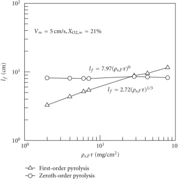
of ρs,Fτ. As shown in Figure 8, the steady flame lengthlf

lf (cm) 102 102 101 101 100 100 First-order pyrolysis Zeroth-order pyrolysis V∞=5 cm/s,XO2,∞=21% ρs,Fτ(mg/cm2₎ lf =7.97(ρ_s,Fτ)0 lf =2.72(ρ_s,Fτ)1/3

Figure 8: Thickness eﬀect on flame length for both pyrolysis

models.

is almost constant for diﬀerent ρs,Fτ in the zeroth-order

pyrolysis model.

On the other hand, as suggested by (6) and (8), burning

rate on the surface for first-order pyrolysis increases with the solid thickness (again, by assuming the pyrolysis temperature

is very close for diﬀerentρs,Fτcases). As a result,lf at steady

state increases with theρs,Fτ as shown inFigure 8. For this

case, the lf dependence on ρs,Fτ is of power 1/3 (lf ∝

(ρs,Fτ)1/3).

3.3.2. Thickness Eﬀect on Spread Rate. One of the important

features of a spreading flame over a solid is the spread rate. When the steady state is reached, by the conservation of solid fuel mass, one can have the following equation (neglecting fuel leftover):

Vfρs,Fτ=m˙. (9)

The computed results show that the total burning rate, ˙m

is proportional to the flame length, lf. Therefore, the Vf

dependence onρs,Fτcan be expressed as follows:

Vf = ˙ m ρs,Fτ ∝ lf ρs,Fτ ∝ ρs,Fτ a−1 , (10)

where a is the power dependence oflf on ρs,Fτ discussed

previously: a ≈ 0 for the zeroth-order pyrolysis model

and a ≈ 1/3 for the first-order pyrolysis model. Vf versus

ρs,Fτ for both solid pyrolysis models are shown inFigure 9.

It is not surprising that the theoretical prediction of the

power dependence ofVf onρs,Fτ coincides nicely with the

numerical results,−1 and−2/3 for the zeroth-order pyrolysis

model and the first-order pyrolysis model, respectively, as shown in the figure.

(8)

10−1 10−2 101 100 102 101 100 First-order pyrolysis Zeroth-order pyrolysis Vf =5 cm/s,X_O2,∞=21% Vf (cm/s) ρs,Fτ(mg/cm2₎ Vf =2.4(ρ_s,Fτ)−1 Vf =0.77(ρs,Fτ)−2/3

Figure 9: Thickness eﬀect on spread rate for both pyrolysis models.

4. Conclusions

Using a two-dimensional, transient, laminar flame spread code, computed steady spreads over thin solids in low-speed concurrent forced flow have been obtained using

two diﬀerent solid pyrolysis models. Comparisons of the

numerical results show many diﬀerences between the

zeroth-order surface pyrolysis and the first-zeroth-order in-depth pyrolysis cases. The following are some of the key findings of this work.

(1) The mass burning rate distributions on the solid

sur-face are qualitatively diﬀerent. For the zeroth-order

pyrolysis, solid pyrolysis occurs on the solid surface only and the fuel vapor mass flux on the surface reaches a maximum value at the fuel burnout point with an abrupt drop to zero upstream. For the first-order pyrolysis, solid decomposition occurs every-where within the solid fuel once being heated. The fuel mass flux on the surface is the accumulation of the local vapor produced inside the solid. The peak of fuel mass flux on the surface occurs in the pyrolysis region. It will not drop to zero within the finite domain of the flame zone.

(2) The nature of the fuel mass flux distribution results in a special leftover fuel phenomenon which is not observed in the zeroth-order pyrolysis model. Due to finite rate gas-phase reaction used in the model, the flame base will adjust its location to find enough fuel vapor. In the zeroth-order pyrolysis model, the flame base always anchors at the solid burnout point where fuel mass flux has the maximum value. On the other hand, in the first-order pyrolysis model, the peak value of fuel mass flux becomes smaller

and its location shifts downstream when the flame approaches the extinction limit. The flame base moves before solid fuel burns out completely thus leaving unburned solid fuel upstream.

(3) Solid fuel thickness eﬀects on the flame length

and the spread rate for each pyrolysis model are

also diﬀerent. In the zeroth-order pyrolysis model,

gaseous flames are essentially the same for diﬀerent

sample thicknesses. The flame length is independent of thickness and the spread rate is approximately inversely proportional to thickness. In the first-order in-depth pyrolysis model, fuel mass flux at the surface increases with thickness, resulting in a longer flame. The computed result shows that flame length increases with thickness with a power dependence of 1/3. The spread rate decreases with thickness with a

−2/3 power dependence.

The present numerical results show that diﬀerent solid

pyrolysis models can have a drastic influence on flame

spreading behavior in concurrent flow. Their eﬀect on

op-posed-flow spread is not yet clear. More sophisticated pyrol-ysis models also need to be tested in the future to assess their influence.

Nomenclature

a: Power dependence of the flame length on the

sample thickness

AI: Solid-phase preexponential factor for the

in-depth pyrolysis model

As: Solid-phase preexponential factor for the surface

pyrolysis model

Cs: Solid-phase-specific heat

EI: Solid-phase activation energy for the in-depth

pyrolysis model

Es: Solid-phase activation energy for the surface

pyrolysis model

ks: Solid-phase-specific heat

L: Latent heat

lf: Flame length

˙

m: Total mass burning rate total (the integration of

˙

mover the solid surface)

˙

m: Mass burning rate or fuel vapor mass flux

˙

q_c_{, in}: Convective heat flux on the solid surface from the

gas-phase ˙

qr,out: Net radiative heat loss from the solid surface

˙

q_net,in: Net heat flux going into the interior of the solid

(=q˙_c_,in−q˙_r_,out−m˙L)

Ru: Universal gas constant

t: Time

Ts: Solid temperature

Ts,w: Solid surface temperature

Vf: Flame spread rate

V∞: Free stream velocity

XO2,∞: Free stream oxygen molar fraction

x: x-coordinate

(9)

y: y-coordinate

ys: y-coordinate for the solid phase

αg: Gas-phase thermal diﬀusivity

ρs: Compound solid density

ρs,F: Solid fuel density

ρs,F0: Initial solid fuel density

τ: Virgin sample thickness

τF: Solid fuel thickness

τF,0: Initial solid fuel thickness

ωF: Fuel vapor consumption rate

ωF,max: Maximum fuel vapor consumption rate at a

certain instant.

Acknowledgment

This research is supported by a grant from NASA Glenn

Research Center monitored by Dr. Gary Ruﬀ.

References

[1] D. Mohan, C. U. Pittman, and P. H. Steele, “Pyrolysis of wood/biomass for bio-oil: a critical review,” Energy and Fuels, vol. 20, no. 3, pp. 848–889, 2006.

[2] R. E. Lyon and R. N. Walters, “Pyrolysis combustion flow calorimetry,” Journal of Analytical and Applied Pyrolysis, vol. 71, no. 1, pp. 27–46, 2004.

[3] C. Lautenberger and C. Fernandez-Pello, “Generalized pyrol-ysis model for combustible solids,” Fire Safety Journal, vol. 44, no. 6, pp. 819–839, 2009.

[4] C. Di Blasi, “Processes of flames spreading over the surface of charring fuels: eﬀects of the solid thickness,” Combustion and Flame, vol. 97, no. 2, pp. 225–239, 1994.

[5] H. C. Kung, “A mathematical model of wood pyrolysis,” Combustion and Flame, vol. 18, no. 2, pp. 185–195, 1972. [6] A. E. Frey and J. S. T’ien, “A theory of flame spread over a

solid fuel including finite-rate chemical kinetics,” Combustion and Flame, vol. 36, pp. 263–289, 1979.

[7] S. Bhattacharjee and R. A. Altenkirch, “Radiation-controlled, opposed-flow flame spread in a microgravity environment,” Proceeding of Combustion Institute, vol. 23, no. 1, pp. 1627– 1633, 1991.

[8] P. V. Ferkul and J. S. T’ien, “A model of low-speed concurrent flow flame spread over a thin fuel,” Microgravity Science and Technology, vol. 99, no. 4–6, pp. 345–370, 1994.

[9] C. B. Jiang, J. S. Tien, and H. Y. Shih, “Model calculation of steady upward flame spread over a thin solid in reduced gravity,” Proceeding of Combustion Institute, vol. 26, no. 1, pp. 1353–1360, 1996.

[10] H. Y. Shih and J. S. T’ien, “A three-dimensional model of steady flame spread over a thin solid in low-speed concurrent flows,” Combustion Theory and Modelling, vol. 7, no. 4, pp. 677–704, 2003.

[11] P. Ferkul, J. Kleinhenz, H. Y. Shih, R. Pettegrew, K. Sack-steder, and J. T’ien, “Solid fuel combustion experiments in microgravity using a continuous fuel dispenser and related numerical simulations,” Microgravity Science and Technology, vol. 15, no. 2, pp. 3–12, 2004.

[12] A. Kumar, H. Y. Shih, and J. S. T’ien, “A comparison of extinction limits and spreading rates in opposed and concurrent spreading flames over thin solids,” Combustion and Flame, vol. 132, no. 4, pp. 667–677, 2003.

[13] Y.-T. Tseng and J. S. T’ien, “Limiting length, steady spread and non-growing flames in concurrent flow over solids,” Journal of Heat Transfer, vol. 132, no. 9, Article ID 091201, 2010. [14] J. S. T’ien, H.-Y. Shih, C.-B. Jiang et al., “Mechanisms of

flame spread and smolder wave propagation,” in Microgravity Combustion: Fire in Free Fall, pp. 299–418, Academic Press, San Diego, Calif, USA, 2001.

[15] M. M. Delichatsios and M. A. Delichatsios, “Eﬀects of tran-sient pyrolysis on wind-assisted and upward flame spread,” Combustion and Flame, vol. 89, no. 1, pp. 5–16, 1992. [16] J. S. T’Ien and M. P. Raju, “Two-phase flow inside an externally

heated axisymmetric porous wick,” Journal of Porous Media, vol. 11, no. 8, pp. 701–718, 2008.

[17] H. R. Baum and A. Atreya, “A model of transport of fuel gases in a charring solid and its application to opposed-flow flame spread,” in 31st International Symposium on Combustion, pp. 2633–2641, deu, August 2006.

[18] A. I. Brown and S. M. Marco, Introduction to Heat Transfer, McGraw-Hill, New York, NY, USA, 3rd edition, 1958. [19] P. C. Lewellen, W. A. Peters, and J. B. Howard, “Cellulose

pyrolysis kinetics and char formation mechanism,” in Pro-ceedings of the 16th International Symposium on Combustion, pp. 1471–1480, 1977.

(10)

International Journal of

Aerospace

Engineering

Hindawi Publishing Corporation

http://www.hindawi.com Volume 2010

Robotics

Journal of

http://www.hindawi.com Volume 2014 Active and Passive Electronic Components

Control Science and Engineering

Journal of

Hindawi Publishing Corporation

http://www.hindawi.com Volume 2014

Machinery

Hindawi Publishing Corporation http://www.hindawi.com

Journal of

Engineering

Volume 2014

Submit your manuscripts at

http://www.hindawi.com

VLSI Design

Hindawi Publishing Corporation

http://www.hindawi.com Volume 2014

http://www.hindawi.com Volume 2014 Shock and Vibration

Civil Engineering

Advances in

Acoustics and VibrationAdvances in

http://www.hindawi.com Volume 2014 Electrical and Computer Engineering

Journal of

Advances in OptoElectronics

Hindawi Publishing Corporation

http://www.hindawi.com Volume 2014

The Scientific

World Journal

Sensors

Journal of

Modelling & Simulation in Engineering Hindawi Publishing Corporation

Chemical Engineering

International Journal of Antennas and

Propagation

Navigation and Observation

Research Article A Comparison of Flame Spread Characteristics over Solids in Concurrent Flow Using Two Different Pyrolysis Models