CUSTOMER segmentation, such as customer grouping by

Improving Personalization Solutions through

Optimal Segmentation of Customer Bases

Tianyi Jiang and Alexander Tuzhilin

Abstract—On the Web, where the search costs are low and the competition is just a mouse click away, it is crucial to segment the customers intelligently in order to offer more targeted and personalized products and services to them. Traditionally, customer segmentation is achieved using statistics-based methods that compute a set of statistics from the customer data and group customers into segments by applying distance-based clustering algorithms in the space of these statistics. In this paper, we present a direct grouping-based approach to computing customer segments that groups customers not based on computed statistics, but in terms of optimally combining transactional data of several customers to build a data mining model of customer behavior for each group. Then, building customer segments becomes a combinatorial optimization problem of finding the best partitioning of the customer base into disjoint groups. This paper shows that finding an optimal customer partition is NP-hard, proposes several suboptimal direct grouping segmentation methods, and empirically compares them among themselves, traditional statistics-based hierarchical and affinity propagation-based segmentation, and one-to-one methods across multiple experimental conditions. It is shown that the best direct grouping method significantly dominates the statistics-based and one-to-one approaches across most of the experimental conditions, while still being computationally tractable. It is also shown that the distribution of the sizes of customer segments generated by the best direct grouping method follows a power law distribution and that microsegmentation provides the best approach to personalization.

Index Terms—Customer segmentation, marketing application, personalization, one-to-one marketing, customer profiles.

Ç

1

I

NTRODUCTION

C

USTOMERsegmentation, such as customer grouping by the level of family income, education, or any other demographic variable, is considered as one of the standard techniques used by marketers for a long time [40]. Its popularity comes from the fact that segmented models usually outperform aggregated models of customer beha-vior [45]. More recently, there has been much interest in the marketing and data mining communities in learning individual models of customer behavior within the context of one-to-one marketing [37] and personalization [8], when models of customer behavior are learned from the data pertaining only to a particular customer. These learned individualized models of customer behavior are stored as parts of customer profiles and are subsequently used for recommending and delivering personalized products and services to the customers [2].

As was shown in [21], it is a nontrivial problem to compare segmented and individual customer models because of the tradeoff between the sparsity of data for individual customer models and customer heterogeneity in aggregate models: individual models may suffer from sparse data, while aggregate models suffer from high levels of customer heterogeneity. Depending on which effect

dominates the other, it is possible that models of individual customers dominate the segmented or aggregated models, and vice versa.

A typical approach to customer segmentation is a distance-measure-based approach where a certain proximity or similarity measure is used to cluster customers. In this paper, we consider thestatistics-basedapproach, a subclass of the distance-measure-based approaches to segmentation that computes the set of summary statistics from customer’s demographic and transactional data [6], [21], [47], such as the average time it takes the customer to browse the Web page describing a product, maximal and minimal times taken to buy an online product, recency, frequency, and monetary (RFM values) statistics [34], and so forth. These customer summary statistics constitute statistical reductions of the customer transactional data across the transactional variables. They are typically used for clustering in the statistics-based approach instead of the raw transactional data since the unit of analysis in forming customer segments is the customer, not his or her individual transactions. After such statistics are computed for each customer, the customer base is then partitioned into customer segments by using various clustering methods on the space of the computed statistics [21]. It was shown in [21] that the best statistics-based approaches can be effective in some situations and can even outperform the one-to-one case under certain condi-tions. However, it was also shown in [21] that this approach can also be highly ineffective in other cases. This is primarily because computing different customer statistics would result in different h-dimensional spaces, and various distance metrics or clustering algorithms would yield different clusters. Depending on particular customer statis-tics, distance functions, and clustering algorithms, signifi-cantly different customer segments can be generated. . T. Jiang is with AvePoint Inc., 3 2nd Street, Suite 803, Jersey City, NJ

07302. E-mail: tjiang@stern.nyu.edu.

. A. Tuzhilin is with the Department of Information, Operations, and Management Sciences, Stern School of Business, New York University, 44 West 4th Street, Room 8-92, New York, NY 10012.

E-mail: atuzhili@stern.nyu.edu.

Manuscript received 22 May 2007; revised 14 Feb. 2008; accepted 15 July 2008; published online 30 July 2008.

For information on obtaining reprints of this article, please send e-mail to: tkde@computer.org, and reference IEEECS Log Number TKDE-2007-05-0230. Digital Object Identifier no. 10.1109/TKDE.2008.163.

In this paper, we present an alternative direct grouping segmentation approach that partitions the customers into a set of mutually exclusive and collectively exhaustive segments not based on computed statistics and particular clustering algorithms, but in terms of directly combining transactional data of several customers, such as Web browsing and purchasing activities, and building a single model of customer behavior on this combined data. This is a more direct approach to customer segmentation because it directly groups customer data and builds a single model on this data, thus avoiding the pitfalls of the statistics-based approach, which selects arbitrary statistics and groups customers based on these statistics.

We also discuss how to partition the customer base into an optimal set of segments using the direct grouping approach, where optimality is defined in terms of a fitness function of a model learned from the customer segment’s data. We formulate this optimal partitioning as a combina-torial optimization problem and show that it is NP-hard. Then, we propose several suboptimal polynomial-time direct grouping methods and compare them in terms of the modeling quality and computational complexity. As a result, we select the best of these methods, called Iterative Merge (IM), and compare it to the standard statistics-based hierarchical segmentation methods [13], [21], to a modified version of the statistics-based affinity propagation (AP) clustering algorithm [15], and to the one-to-one approach. We show thatIMsignificantly dominates all other methods across a broad range of experimental conditions and different data sets considered in our study, thus demon-strating superiority of the direct grouping methods to profiling online customers.

We also examine the nature of the segments generated by theIMmethod and observe that there are very few size-one segments, that the distribution of segment sizes reaches its maximum at a very small segment size, and that the rate of decline in the number of segments after this maximum follows a power law distribution. This observation, along with the dominance of IM over the one-to-one method, provides support for the microsegmentation approach to personalization [24], where the customer base is partitioned into a large number of small segments.

In summary, we make the following contributions in this paper:

. Propose the direct grouping method for segmenting customer bases, formulate the optimal segmentation problem, and show that it is NP-hard.

. Propose several suboptimal direct grouping meth-ods, empirically compare them, and show that the direct grouping method IMsignificantly dominates others.

. Adapt a previously proposed AP clustering algo-rithm [15] to the statistics-based customer segmenta-tion problem and show that it dominates several existing statistics-based hierarchical clustering (HC) methods.

. CompareIMagainst the statistics-based hierarchical segmentation,AP, and theone-to-oneapproaches and demonstrate that IM significantly dominates them. This is an important result because it demonstrates

that, in order to segment the customers, it is better to first partition customer data and then build pre-dictive models from the partitioned data rather than first compute some arbitrary statistics, cluster the resulting h-dimensional data points into segments, and only then build predictive models on these segments.

. Plot the frequency distribution of the sizes of customer segments generated by the IM method and show that the tail of this plot follows a power law distribution. This means that IM generates many small customer segments and only few large seg-ments. This result provides additional support for the microsegmentation approach to personalization. The rest of this paper is organized as follows: In Section 2, we present our formulation of the optimal direct grouping problem. We review the current literature on related work in Section 3. In Section 4, we discuss our implementations of two statistics-based segmentation methods, our adaptation ofAPas a statistics-based segmentation method,one-to-one segmentation, and three suboptimal direct grouping meth-ods. In Section 5, we lay out our experimental setup and discuss the results in Sections 6. In Section 7, we provide more detailed analysis.

2

P

ROBLEM

F

ORMULATION

The problem of optimal segmentation of a customer base into a set of mutually exclusive and collectively exhaustive set of customer segments can be formulated as follows: Let C be the customer base consisting of N customers, each customer Ci is defined by the set of m demographic

attributesA¼ fA1; A2;. . .; Amg,kitransactionsT ransðCiÞ ¼

fT Ri1; T Ri2;. . .; T Rikig performed by customer Ci, and h summary statistics Si¼ fSi1; Si2;. . .; Sihg computed from

the transactional dataT ransðCiÞ that are explained below.

Each transaction T Rij is defined by a set of transactional

attributesT¼ fT1; T2;. . .; Tpg. The number of transactionski

per customer Ci varies. Finally, we combine the

demo-graphic attributes fAi1; Ai2;. . .; Aim;g of customer Ci and

his/her set of transactionsfT Ri1; T Ri2;. . .; T Rikig into the complete set of customers’ data T AðCiÞ ¼ fAi1; Ai2;. . .; Aim; T Ri1; T Ri2;. . .; T Rikig, which constitutes a unit of analysis in our work. As an example, assume that customer Ci can be defined by attributes A¼ fName;Age;Income;

and other demographic attributesg, and by the set of pur-chasing transactions T ransðCiÞ she made at a website,

where each transaction is defined by such transactional attributes T as an item being purchased, when it was purchased, and the price of the item.

Summary statistics Si¼ fSi1; Si2;. . .; Sihg for customer

Ci is a vector in anh-dimensional euclidean space, where

each statistics Sij is computed from the transactions

T ransðCiÞ ¼ fT Ri1; T Ri2;. . .; T Rikig of customer Ci using various statistical aggregation and moment functions, such as mean, average, maximum, minimum, variance, and other statistical functions. For instance, in our previous example, a summary statistics vectorSican be computed across all of

the customerCi’s purchasing sessions and can include such

session, the average number of items bought, and the average time spent per online purchase session. This means, among other things, that each customer Ci has a unique

summary statistics vector Si and that a customer is

represented with a unique point in the euclidean space of summary statistics.1

Given the set of N customers C1;. . .; CN, and their

respective customer data p¼ fT AðC1Þ;. . .; T AðCNÞg, we

want to build a single predictive modelMon this group of

customersp:

Y ¼f^ðX1; X2;. . .; XpÞ; ð1Þ

where dependent variableY constitutes one of the transac-tional attributesTjand independent variablesX1; X2;. . .; Xp

are all the transactional and demographic variables, except variable Tj, i.e., they form the set T[ATj. The

perfor-mance of model M can be measured using some fitness

function f mapping the data of this group of customersp

into reals, i.e.,fðpÞ 2 <.

For example, model M can be a decision tree built on

data p of customers C1;. . .; CN, for the purpose of

predicting Tj variable “time of purchase” using all the

transactional and demographic variables, except variableTj

(i.e., T[ATj) as independent variables. The fitness

function f of model M can be its predictive accuracy on

the out-of-sample data or computed using 10-fold cross validation.

The fitness functionfcan be quite complex in general, as it represents the predictive power of an arbitrary predictive modelMtrained on all customer data contained inp. For

example,f could be the relative absolute error (RAE) of a neural network model trained and tested onp via 10-fold

cross validation for the task of predicting time of the day of a future customer purchase. Given that fitness functionfis a performance measure of an arbitrary predictive model, in general, functionfdoes not have “nice” properties, such as additivity or monotonicity. For example, fðfT AðCiÞgÞ can

be greater than, less than, or equal tofðfT AðCiÞ; T AðCjÞgÞ

for anyi,j.

We next describe the problem of partitioning the customer base C into a mutually exclusive collectively exhaustive set of segments P ¼ fp1;. . .; pg and building

modelsMof the form (1) for each segmentp, as described

above. Clearly, customers can be partitioned into segments in many different ways, and we are interested in an optimal partitioning that can be defined as follows:

Optimal customer segmentation (OCS) problem. Given the customer base C of N customers, we want to partition it into the disjoint groups P¼ fp1;. . .; pg, such that the

models M built on each group p would collectively

produce the best performance for the fitness functionfðpÞ

taken over p1;. . .; p. Formally, this problem can be

formulated as follows: Let be a weighting measure

specifying “importance” of segment. Some examples of

include simple average 1= and proportional weights jT AðpÞj=jT AðCÞj. Then, we want to find a partition of the

customer base C into the set of mutually exclusive collectively exhaustive segments P ¼ fp1;. . .; pg, where

segmentp is defined by its customer data p¼ fT AðCjÞ;

. . .; T AðCmÞg, such that the following fitness score

’¼X

¼1

fðpÞ

is maximized (or minimized if we used error rates as our fitness score) over all possible partitions P ¼ fp1;. . .; pg,

such that p\p¼ ; and [p¼P. Note that different

predictive tasks (i.e., predicting different transactional variables) result in different optimal partitions of the customer baseC.

Clearly, the OCS is acombinatorial partition problem[20], and it is computationally hard, as the following proposition shows.

Proposition.OCS problem is NP-hard.

Sketch of Proof.This result can be obtained by reducing the clustering problem, which is NP-hard [7], to the OCS

problem. tu

Since the OCS problem is NP-hard, we propose some suboptimal polynomial time methods that provide reason-able performance results. More specifically, we consider the following three types of customer segmentation methods as approximations to the solution of the OCS problem:

. Statistics based—This traditional customer segmenta-tion approach groups customers by first computing some statisticsSi¼ fSi1; Si2;. . .; Sihgfor customerCi

from that customer’s demographic and transactional data, considers these statistics as unique points in an h-dimensional space, groups customers into seg-mentsP ¼ fp1;. . .; pg by applying various

cluster-ing algorithms to these h-dimensional points, and then builds models M of the form (1) for each

segment p, as described above. Note that this

method constitutes a subset of the distance-mea-sure-based segmentation approach described in Section 3 below.

. One-to-one—The basis for one-to-one approach is that each individual customer exhibits idiosyncratic behavior and that the best predictive models of customer behavior are learned from the data pertaining only to a particular customer. Rather than building customer segments of various sizes, the one-to-one approach builds customer segments of size 1, which is just the customer him/herself.

. Direct grouping—Unlike the traditional statistics-based approach to segmentation, the direct group-ing approach directly groups customer data into segments for a given predictive task via combina-torial partitioning of the customer base (without clustering them into segments using statistics-based or any other distance-based clustering methods). Then, it builds asinglepredictive model (1) on this customer data for each segment and uses the aforementioned fitness score to derive the decisions on how to do the combinatorial partitioning of the customer base. The direct grouping method avoids the pitfalls of the statistics-based approach, which selects and computes an arbitrary set of statistics out

1. This observation will be extensively used later when hierarchical clustering methods are introduced in Section 4 and beyond.

of a potentially infinite set of choices. Since segmentation results critically depend on a good choice of these statistics, the statistics-based ap-proach is sensitive to this somewhat arbitrary and highly nontrivial selection process, which the direct grouping approach avoids entirely. Instead of looking for an optimal grouping of customers, which was shown above to be NP-hard, we will present three polynomial-time suboptimal direct grouping methods in this paper.

Before we describe these methods in more detail, we first present some of the related work.

3

R

ELATED

W

ORK

The problem of finding the global optimal partition of customers is related to the work on 1) combinatorial optimization problems in operations research, 2) customer segmentation in marketing, and 3) data mining and user-modeling research on customer segmentation. We examine the relationship of our work to these three areas of research in this section.

3.1 Combinatorial Optimization

Combinatorial optimization models are used across a wide range of applications. Combinatorial optimization problems are in general NP-hard; however, depending on the mathematical formulation of a particular problem, near-optimal approximations to exact solutions can be achieved in polynomial time [20]. Despite recent advances in finding solutions to various combinatorial optimization problems, there is still a large set of problems considered too complex to derive optimal or near-optimal solutions [20]. Therefore, various heuristics were explored in obtaining good solu-tions that have no guarantees as to their “closeness” to the optimal solution, including greedy hill climbing [27], simulated annealing [18], evolutionary algorithms [32], and neural networks [4].

Our OCS problem falls in this category of “hard” problems because we cannot use any existing problem formulations to solve it due to the dependence of the fitness function f on data in p in a complicated manner that

precludes various useful characterizations of the fitness function, such as having additivity, monotonicity, and other “nice” properties. Therefore, in our work we do not explore any of the near-optimal solutions and deploy the greedy hill-climbing approach instead in conjunction with a branch-and-bound enumerative technique in developing our fitness function-based methods.

3.2 Customer Segmentation in Marketing

Customer segmentation has been extensively studied by marketers since the time Smith introduced the concept of segmentation back in 1956 [40]. Its popularity comes from the fact that segmented models usually outperform aggregated models of customer behavior [45]. In particular, marketers classify various segmentation techniques into a priori versus post hoc anddescriptiveversuspredictivemethods giving rise to a 2 2 classification matrix of these techniques [45]. Among various segmentation methods studied in the marketing literature, the ones that are most closely related

to our work are various clustering techniques, mixture models, (generalized) mixture regression models, and continuous mixing distributions.

Clustering methods are classified into nonoverlapping methods, when customer can belong to only one segment, overlapping methods, when customer can belong to more than one segment, and fuzzy methods, when customers can belong to different segments with certain probabilities [45]. From this perspective, we assume the nonoverlapping model in our clustering approaches in which customers belongonly to onesegment.

Much segmentation work in marketing pertains to the mixture models where observation is a random variable that follows a probability density function conditional on the observation belonging to segments. Also, DeSarbo and Cron [11] present a mixture regression model and Wedel and DeSarbo [43] present the generalized mixture regression model that add to these mixture model the fact that the means of the observations in each segment depend in the form of a linear regression on a set of explanatory variables. This means that each segment is defined by its own regression model with the set of parameters unique for that segment.

Furthermore, Allenby and Rossi [3], Wedel et al. [44], and others extended these segmentation-based mixture models to the continuous distribution models where each customer has a set of density distribution parametersunique for that customer rather than for the segment to which the customer belongs. Subsequently, Allenby and Rossi [3] used hierarchical Bayesian methods to model these continuous distributions and MCMC simulation methods to estimate unique parameters for each customer. It was shown empirically in [3] that this approach outperformed finite mixture segmentation models, thus providing evidence to the advantages of individual customer modeling.

Our work differs from this previous research in market-ing in that we have proposed the direct groupmarket-ing approach to segmentation that is based on the combinatorial parti-tioning of the customer base rather than on finite mixture, continuous distribution, or clustering methods used by marketers. Although Spath [41] describes a clusterwise linear regression approach that form a partition of lengthK and corresponding sets of parametersbk, such that the sum

of the error sums of squares computed over all clusters is minimized, seems similar to ourdirect groupingapproach, it is actually very different in that it considers each customer as a single observation point to be clustered with other customers. In contrast, in ourdirect groupingapproach, each customer is represented by a group of observation points that is his/her own set of purchase transactions.

In this paper, we compare the direct grouping approach with the previously studied statistics-based and one-to-one segmentation methods and demonstrate that the best grouping-based segmentation method outperforms the one-to-one and the traditional clustering methods, and that the segment size distribution generated by this method follows a power law distribution, which is a linear distribution on a log-log plot that are used to describe naturally occurring phenomena such as word frequencies, income, city sizes, and so forth. In our case, our results show that large segment sizes are rare, whereas small segment sizes are very common.

3.3 Customer Segmentation in Data Mining

More recently, there has been much interest in the data mining and user modeling communities in learning indivi-dual models of customer behavior within the context of personalization [2], [8], when models of customer behavior are learned from the data pertaining only to a particular customer. One stream of research in user modeling pertains to building user profiles [1], [35], [36]. For example, in [36], a user profile is defined as a vector of weights for a set of certain keywords. Moreover, customer profiles can be defined not only as sets of attributes but also as sets of rules defining behavior of the customer [1], sets of sequences such as sequences of Web browsing activities [17], [31], [42], and signatures used to capture the evolving behavior learned from data streams of transactions [10]. There has also been some work done on modeling personalized customer behavior by building appropriate probabilistic models of customers. For example, Cadez et al. [9] build customer profiles using finite mixture models and Manavoglu et al. [29] use maximum entropy and Markov mixture models for generating probabilistic models of customer behavior. Finally, Nasraoui et al. [33] describe how to mine evolving user profiles and use them in recommender systems in order to build relationships with the customers.

Our work is also related to the work on clustering that partitions the customer base and their transactional histories into homogeneous clusters for the purpose of building better models of customer behavior using these clusters [5], [6], [16], [21], [25], [26], [28], [39], [47]. These clustering methods use distance-measure-based metrics to compute “distances” between individual customers and group customers into clusters based on these distances. These distances between customers can be defined in various ways. For example, Guha et al. [16] describe an HC approach, ROCK, which clusters customers based on the distance between them, where the distance between two customers is defined in terms of how “similar” the two sets of their transactions are. Thus, Guha et al. [16] reduce the customer segmentation problem to finding clusters in weighted graphs and use an HC method for finding the segments. Boztug and Reutterer [5] and Reutterer et al. [39] address the problem of segmenting customers having multiple shopping basket transactions. This segmentation is achieved by, first, creating K shopping basket prototypes from the set of all shopping transactions from all customers using a variant of the K-means clustering method. Then, individual customers are assigned to the closest basket prototype based on a certain distance measure between the set of customer’s transactions and the prototype. This method is highly scalable but assumes a certain fixed number of prototype baskets in defining potential customer segments. Malthouse [28] introduces the concept of subsegmentation, where custo-mers from the same market segment are further partitioned into subsegments using such criteria as RFM values. Then, customers in the same subsegment are targeted with customized offerings. Furthermore, Koyuturk et al. [25] and Leisch [26] present certain clustering approaches based on a variant of a Semidiscrete Decomposition (SDD) and on thek-centroid method, respectively, which are particularly well suited for clustering high-dimensional data sets and can also be used for segmenting customer bases.

Another way to segment the customers using distance-measure-based clustering methods is to compute a set of statistics from the customer’s transactional and demo-graphic data, map each customer into an h-dimensional space, and use standard clustering methods to segment the customers. In Section 1, we called it the statistics-based approach, and it was also deployed in [6], [21], and [47]. In particular, Brijs et al. [6] compute statistics from customer’s transactional and demographic data and use clustering methods to partition the customers into groups. Also, Yang and Padmanabhan [47] use pattern-based and association mining methods to cluster customers’ transactions. Both Brijs et al. [6] and Yang and Padmanabhan [47] cluster customers into groups but do not build customer models on these groups. In contrast to this, Jiang and Tuzhilin [21] cluster customers into groups using HC methods and build predictive models on individual groups. One of the problems with the statistics-based methods from [6], [21], and [47] is that they deploy somewhat arbitrary set of statistics and that it is difficult to construct an objective and truly superior measure of intracluster similarity and intercluster dissimilarity for the segmentation problems considered in this paper. Therefore, it is not surprising that it was shown in [21] that the statistics-based approaches produced mixed performance results.

In summary, the personalization approaches developed in the data mining and user-modeling communities focus on the task of building good profiles and models of customers but do not consider direct grouping methods, do not study optimal or suboptimal customer segmentation strategies, and do not compare direct grouping against one-to-one and statistics-based segmentation methods. In this paper, we focus on the direct grouping methods and empirically compare their performance against the statis-tics-based and one-to-one approaches.

4

S

EGMENTATION

A

PPROACHES TO

B

UILDING

P

REDICTIVE

M

ODELS OF

C

USTOMER

B

EHAVIOR

In this section, we describe the details of the statistics-based, one-to-one, and direct grouping approaches before empiri-cally comparing them across various experimental settings. We would like to reiterate that the statistics-based and the direct grouping methods only partition the customers into different segments. Once the segments are formed, we next build predictive models of type (1) on these segments and measure the overall performance of these models across the segments using the fitness function’.

4.1 Statistics-Based Segmentation Methods

In terms of the statistics-based segmentation, we consider the following two variants of the hierarchical approach that are described in [13] and [19] and deployed in [21] and [35] and an adaptation of a previously proposed statistics-based methodAP[15] to our segmentation problem.

HC: Using the same top-downHCtechniques as in [21], we learn predictive models of customer behavior of the form (1) defined in Section 2, i.e.,

where X1; X2;. . .; Xp are some of the demographic

attri-butes fromAand some of the transactional attributes from T (see Section 2), and function f^is a model that predicts certain characteristics of customer behavior, such as prediction of the product category or the time spent on a website purchasing the product. The correctness measure of this prediction is our fitness function f (as defined in Section 2).

In the context ofHC, predictive modelsMof the form (1)

are learned on the groups of customersp, which are formed

as follows. First, each customerCiis mapped into the space of

summary statisticsSi¼ fSi1; Si2;. . .; Sihgthat are computed

from the transactional data T ransðCiÞ of customer Ci as

explained in Section 2. Therefore, each customerCibecomes

a single vector point in anh-dimensional euclidean space, andNcustomers in the customer baseCresult inNpoints in this space. Given these N points in the h-dimensional summary statistics space Si, the customer segments are

formed by applying unsupervised clustering methods to that space. The distance between two points (customers) is defined as a euclidean distance between the two vectors. Further, we use distance-basedHCmethod that starts with a single segment containing all the N customers in the customer base C and generates new levels of segment hierarchy via progressively smaller groupings of customers until the individual customer (one-to-one) level is reached containing only single customers. In our particular imple-mentation ofHC, we have chosen FarthestFirst [19], a greedy k-center unsupervised clustering algorithm that is found to perform well in [21] on customer summary statistics and demographics attributes fA1; A2;. . .; Am; S1; S2;. . .; Shg.

FarthestFirst generates progressively smaller customer seg-ments for each level of the segmentation hierarchy starting from the single segmentCand going down to the one-to-one level. Moreover, for each level L of the segmentation hierarchy, FarthestFirst computes the weighted sum of fitness scores, as described in Section 2.

Once theHCmethod computes customer segmentspfor

each level of the segmentation hierarchy, predictive models M of the form (1) are learned on these segments p, as

described above. More specifically, we build predictive modelsM on each customer segmentp for a selective set

of dependent variables as described in Section 2 and collect the fitness scores of these models. Then, the segmentation level with the highest overall fitness score (besides the one-to-one level) is selected as the best possible segmentation of the customer base. Note that while the segments remain fixed after running theHCalgorithm, different models are built for different prediction tasks to make predictions of specific dependent variable, different set of fitness score are computed for these prediction tasks, and different best segmentation levels are selected. As we will discuss in Section 5, we conduct different predictive tasks across different experimental condition in order to ensure the robustness of our findings and that our results are not due to idiosyncratic behavior of one specific transaction vari-able, prediction task, or data set.

Entropy clustering (EC). Instead of forming different groupings of customer transactions from unsupervised clustering algorithms, as HC does, EC forms customer groupings by building a C4.5 decision tree on customer

summary statistics and demographics fA1; A2;. . .; Am;

S1; S2;. . .; Shg, where the class label is the model’s dependent

variableY in (1). UnlikeHC, this approach is a supervised clustering algorithm, where “similar” customers are grouped in terms of summary statistics and demographics to reduce the entropy of the class label. Thus, for different predictive task, where the dependent variable varies, we generate different decision trees where each end node of the tree constitutes a customer segment. Once the C4.5 forms the groupings based on the principle of class label entropy minimization, we store the fitness scores (e.g., percent correctly classified, RAE, area under ROC curve, and so forth) generated byf^in (1) across these different groupings of customer transaction data for comparison against other segmentation methods. Intuitively, this should be a better approach to clustering customers than HC because by making grouping decisions based on class label purity, we are in effect measuring similarity in the output space, which reduces the variance of the dependent variableYclassified by our predictive models. In addition, there is no fixed splitting factor as in the case ofHC, as each tree split is based on the number of different values an independent attribute may have. Thus, each split could result in a different number of subclusters, which could provide extra flexibility for building more homogeneous and better performing customer seg-ments. However, the formation of customer groups is still based on customer summary statistics, which, depending on the types of statistics used, can yield very different decision trees. Note that for different predictive tasks, because we use different dependent variables as the class label, different segments are generated from different decision trees.

AP. Starting withnunique customers,AP[15] identifies a set of training points, exemplars, as cluster centers by recursively propagating “affinity messages” among train-ing points. Similar to the prototype-generattrain-ing greedy K-medoids algorithms [23],APpicks exemplars as cluster centers during every iteration, where each exemplar in our study isa single customer, represented by his/her summary statistics vector, and forms clusters by assigning an individual exemplar’s group membership based on “affi-nities” that exemplar has with any possible cluster centers. Affinity in our study is defined as pairwise euclidean distance measures an exemplar has with any possible cluster centers. Like other statistics-based methods, we also use summary statistics vectors to represent customers. This reduces the complexity of affinity calculation to that of distances between two customer’s summary statistics vectors. AP runs in Oðn2_{Þ. It is a good method for} segmenting customers because cluster centers are asso-ciated with real customers rather than “virtual” computed customers as in the case of standard clustering algorithms. Again, similar to EC, AP generates different set of customer segments for different predictive tasks as the summary statistics of the dependent variable are not used for clustering.

4.2 One-to-One Method

As explained in Section 2, the one-to-one approach builds predictive models of customer behavior only from individual customer’s transactional data. In other words, for each predictive task (e.g., making prediction on a specific

transac-tional variable), we build a predictive model (1) for each customerCi,i¼1;. . .; N, using only the demographic and

the transactional data of that customer minus the specific transactional variable used as dependent variable in the predictive task. Since this is individual level modeling, we do not have to deal with customer grouping at all in this case.2 For each model of customerCi, we compute fitness function

fðCiÞ(e.g., using 10-fold cross validation with a Naı¨ve Bayes

classifier on T AðCiÞ) and obtain the entire distribution of

these fitness scores (e.g., RAE or the area under the ROC curve) for i¼1;. . .; N. These average predictive perfor-mance score distributions are then stored for later distribu-tion comparisons against scores generated by predictive models evaluating segments formed by other segmentation methods.

4.3 Direct Grouping Methods

The direct grouping approach makes decision on how to group customers into segments by directly combining different customers into groups and measuring the overall fitness score as a linear combination of fitness scores of individual segments, as described in Section 2. Since the optimal segmentation problem is NP-hard (as shown in Section 2), we propose three suboptimal grouping methods Iterative Growth (IG), Iterative Reduction (IR), andIMthat we describe in this section.

IG. We propose the following greedy IGapproach that starts from a single customer and grows the segment one customer at a time by adding the “best” and removing the

“weakest” customer, if any, at a time until all the nonsegmented customers have been examined. More specifically, IG iteratively grows individual customer groups by randomly picking one customer to start a customer group and, then, tries to add one new customer at a time by examining all customers that have not been assigned a group yet. If augmenting a new customer to a group improves the fitness score of the group, then IG examines all existing customers in the group and decides whether or not to exclude one “weakest” customer member to improve the overall group fitness. As a result, only customers not lowering the performance of the group will be added, and the worst performing customer, if any, will be removed from the group, where performance is defined in terms of the fitness function described in Section 2.

Unlike the previous statistics-based methods, where the fitness score distributions stored are from the result of 10-fold cross validations, in direct grouping methods, because the fitness score are used to determine the formation of groupings, we use a separate holdout set to test the predictive models built on the finalized customer segments. This out of sample testing alleviates the problem of over-fitting. Also note that as in the case ofECandAP, for different predictive tasks, where different transaction variables are used as the dependent variable, we generate different set of segments by optimizing different predictive performance objectives specific for that predictive task at hand. The specifics of theIGalgorithm are presented in Fig. 1.

It is easy to see that IG runs in Oðn3_{Þ because for the} group oficustomers it takesnichoices to add the best new customer to the group and i choices to remove the weakest customer from it, resulting inðniÞiiterations for each step of the outer loop in Fig. 1.

While this approach does not exhaustively explore all possible combinations of customer partitions, it does focus on meaningful partitions via a branch and bound heuristic.

2. One of the consequences of building predictive models for individual customers is the necessity to have enough transactional data for that customer. For example, if we want to do 10-fold cross validation to compute predictive performance of such a model, a customer should have at least 10 transactions. In case a customer has too few transactions (e.g., less than 10 in our experiments), we group that customer with a couple of other similar customers in order to have a critical mass of transactions (e.g., at least 10 in our experiments).

The drawback ofIGis that any particular customer group’s fitness score may not improve until it grows to a certain “critical mass” of a sufficient number of customer purchas-ing transactions exhibitpurchas-ing “similar” purchase behavior to train a good predictive model. In addition, once a growing customer group passes a certain “mass,” any single customer’s transaction may not impact the overall perfor-mance of the group enough to be considered for rejection or exclusion, which could result in large customer segments having mixed performance results.

IR. To address the “critical mass” problem of IG, we propose a top-down IR approach where we start with a single group containing all the customers and eliminate the weakest performing customer one at a time until no more performance improvements are possible. Once IR finishes this customer elimination process, it will form a segment out of the remaining customers, group all the eliminated customers together into one residual group, and try to reduce it using the same process. The underlying assump-tion in IR is that there exists a fixed number of ideal customer groupings and that we can narrow down to these grouping by removing one member customer at a time from an aggregate group based on the fitness scores.IRis greedy in that once it reduces the initial customer group to a

smallest best performing group, it will remove that group from further considerations. The specifics of the IR algorithm are presented in Fig. 2.

IRruns inOðn2_{Þbecause, in the worst-case scenario, the} outer loop runs n times, and each time the inner loop examines each of the remaining icustomers for exclusion. As in the case ofIG, we observed from our empirical results presented in Section 5 that IR is also prone to producing large suboptimal customer segments, as the removal of a single customer’s transactions may not significantly affect the performance of large customer segments.

IM. Rather than adding or removing a single customer’s transactions at a time, IM seeks to merge two existing customergroupsat a time. Starting with segments contain-ing individual customers, this method combines two customer segmentsSegA andSegB, when 1) the predictive model based on the combined data performs better and 2) combiningSegA with any other existing segments would

have resulted in a worse performance than the combination of bothSegA andSegB.IMis greedy because it attempts to find the best pair of customer groups and merge them together resulting in the best merging combination. The specifics of theIMalgorithm are presented in Fig. 3.

IM runs in Oðn3_{Þ in the worst case because a single} merge of two groups takesOðn2_{Þtime in the worst case, and} there can be up ton of such merges. In comparison toIG, the search space ofIMis smaller because it merges groups, not individual customers, at a time, and the results reported in Section 6 confirm this observation.

Finally, unlike IG and IR, close examination of our empirical results in Section 5 show thatIM tends to make merging decisions on customer segments of comparable sizes, where each customer segment under merging con-sideration can significantly affect the performance of the merged segments, thus lessen the chance of building large and poorly performing customer segments. This observa-tion provides an intuitive explanaobserva-tion whyIMoutperforms IGandIRmethods, as reported in Section 6.

5

E

XPERIMENTAL

S

ETUP

To compare the relative performance of direct grouping, statistics-based, and one-to-one approaches, we conduct

Fig. 2.IRalgorithm.

pairwise performance comparisons using a variant of the nonparametric Mann-Whitney rank test [30] to test whether the fitness score distributions of two different methods are statistically different from each other. We conduct these performance comparisons across various direct grouping and statistics-based approaches that includeIG,IR,IM,HC, EC, andAPmethods. To ensure robustness of our findings, we set up the pairwise comparisons across the following four dimensions.

Types of data sets. In our study, we worked with the following data sets.

a. Two “real-world” marketing data sets containing panel data3 of online browsing and purchasing activities of website visitors and panel data on beverage purchasing activities of “brick-and-mor-tar” stores. The first data set contains ComScore data from Media Metrix on Internet browsing and buying behaviors of 100,000 users across the US for a period of six months (available via Wharton’s RDS at http://wrds.wharton.upenn.edu/). The second data set contains Nielsen panelist data on beverage shopping behaviors of 1,566 families for a period of one year. The ComScore and Nielsen marketing data sets are very different in terms of the type of purchase transactions (Internet versus physical purchases), variety of product purchases, number of individual families covered, and the variety of demographics. Compared to Nielsen’s beverage purchases in local supermarkets, ComScore data set covers a much wider range of products and demographics and is more representative of today’s large marketing data sets.

We further split these two real-world data sets into four data sets of ComScore high- and low-volume customers, which represent the top and bottom 2,230 customers in terms of transaction frequencies, respectively. Similarly, Nielsen high- and low-volume customer data sets were generated using the top and bottom 156 customers in terms of transaction frequencies, respectively.

b. Two simulated data sets representing high-volume customers (Syn-High) and low-volume customers (Syn-Low), respectively, where within each data set, customer differences are defined by generating different customer summary statistics vector Si for

each customeri. All subsequent customer purchase data are generated from the set of summary statistics vectors Si. These two data sets were generated as

follows: 2,048 unique customer summary statistics were generated by sampling from ComScore custo-mer summary statistics distributions, which is then used to generate the purchase transactions with four transactional variables. The number of transactions per customer is also determined from ComScore customer transaction distributions. This data set is used to better simulate real-world transactional data sets.

Since for the ComScore and Nielsen we consider two data sets (each having high- and low-volume customers), this means thatwe use six data sets in totalin our studies. Some of the main characteristics of these six data sets are presented in Table 1. In particular, CustomerType column specifies the transaction frequency of these data sets, High means that customers perform many transactions on average, while Low means only few transactions per customer. The columns “Percentage of Total Population,” “Families,” and “TotalTransactions” specify the percentage of total data population, the number of families, and the sample family transactions contained in the sample data sets.

Types of predictive models.Due to computational expenses of the model-based methods, we build predictive models using two different types of classifiers via Weka 3.4 system [46]: C4.5 decision tree [38] and Naı¨ve Bayes [22]. These are chosen because they represent popular and fast-to-generate classifiers, which is a crucial criterion for us, given that we have built millions of models in making segment merging decisions and stored 105,626 models for the final holdout set evaluation in our study.

Dependent variables. We built various models to make predictions on different transactional variables, T Rij, to

ensure the robustness of our findings, and we also compare the discussed approaches across different experimental settings. Examples of some of the dependent variables are day of the week, product price, category of website in ComScore data sets, and category of drinks bought, total price, and day of the week in the Nielsen data sets. Note

3. Panel data [24], also called longitudinal or cross-sectional time series data, when used in the context of marketing means that the data about a preselected group of consumers on whom a comprehensive set of demographic information is collected is also augmented with the complete set of their purchases. Therefore, these panel data provide a comprehensive view of purchasing activities of a preselected panel of consumers.

TABLE 1

that, while we did not use all the available transactional variables for testing due to time constraints, we feel that the selected six transactional variables used represent enough of a variation to ensure robust results. Also, for any given predictive task where we useTijas the dependent variable,

the data we used to train any one model are customerCi’s

independent variablesX1; X2;. . .; Xp, exceptT Rij.

Note that for every transactional variable for which we want to make predictions using the direct grouping approach, we generate a new set of segments with various segmentation methods, build models on the final segments, and collect the performance measures produced by those predictive models. Also, we create a training set by randomly drawing out 90 percent of our data in building the segments and then evaluate the final quality of the segments generated by the direct grouping methods on the remaining 10 percent of our data as the separate holdout set in order to avoid overfitting.

Performance measures.We use the following performance measures: percentage of correctly classified instances (CCIs), root mean squared error (RME), and RAE [46].

Given models and , is considered “better” than only when it provides better classification resultsandfewer errors, i.e., when ðCCI>CCIÞ ^ ðRME<RMEÞ ^

ðRAE<RAEÞ. This is the fitness function that we use

only in direct groupingmethods to make segment merging or splitting decisions during the iterative search for the best performing segments. For example, if we add a new customer to a segment in theIGapproach, we check if the expanded segment is better than the initial segment, where “better” is defined in terms of the conjunctive expression specified above.

To compare predictive performance of various methods against HC, we select the best performing segment level generated by HC for CCI, RME, and RAE distributions separately based on the most right skewed CCI distribution and left skewed RME and RAE distributions. To compare the performances of different segmentation methods, such as HC,IM, and so forth, we take distributions of identical performance measures (e.g., CCI) across all the segments generated by these methods and statistically test the null hypothesis that the two distributions are not equal. The specifics of this comparison process are discussed further in Section 6.

In terms of data preprocessing, we discretized our data sets to improve classification speed and performance [12]. Nominal transaction attributes, such as product categories, were discretized to roughly equal representation in sample data to avoid overly optimistic classification due to highly skewed class priors. We also discretized continuous valued attributes such as price and Internet browsing durations based on entropy measures via our implementation of Fayyad’s [14] recursive minimal entropy partitioning algorithm.

As was stated before, the goal of this paper is to determine the best performing segmentation method. To reach this goal, we first compared all three methodsIG,IR, andIMin order to determine the bestdirect groupingapproach. Due to compu-tational expenses of the proposed direct grouping methods, we have done it for all six data sets and all three performance measures, but only for one dependent variable and using

only one classifier (C4.5). We then compared statistics-based segmentation methods HC, EC, and AP across multiple dependent variables, classifiers, and all six data sets to select the best one. After that, we conducted additional experi-ments comparing the best performing direct grouping-based against the best performing statistics-based and theone-to-one methods across multiple classifiers, dependent variables, and all six data sets to identify the best performing method. The results of these comparisons are reported in Section 6.

6

E

MPIRICAL

R

ESULTS

In this section, we present our empirical findings. As mentioned in Section 5, we compare the distribution of performance measures generated by considered predictive models across various experimental conditions. Since we make no assumptions about the shape of the generated performance measure distributions and the number of sample points generated by different segmentation ap-proaches, we use a variant of the nonparametric Mann-Whitney rank test [30] to test whether the distribution of performance measures of the one method is statistically different from another method. For example, to compare HCagainst theone-to-onemethod for the CCI measure, we select the distribution of the CCI measure generated for the best segmentation level of the HC taken across various segments and the distribution of the CCI measure obtained for each individual customer and then apply the Mann-Whitney rank test to compare the two distributions.

The null hypothesis for comparing distributions gener-ated by methods A and B for a performance measure is given as follows:

. (I) H0: The distribution of a performance measure generated by method A is not different from the distribution of the performance measure generated by method B.

. H1þ: The distribution of a performance measure generated by method A is different from the distribution of the performance measure generated by method B in thepositivedirection.

. H1: The distribution of a performance measure generated by method A is different from the distribution of the performance measure generated by method B in thenegativedirection.

To test these null hypotheses across distributions of performance measures generated by different methods, we proceeded as follows: For each data set, classifier, and dependent variable, we generate six sets of customer groups, CG1;. . .; CG6, from our six segmentation methodsIG,IR,IM, HC,EC, andAP, wherecgij denotes a particular groupjof

customers belonging to customer group setCGigenerated by

methodi(IG,IR,IM,HC,EC, orAP). For eachcgij;, we generate

a separate model,mij, that predicts the dependent variable of

the model via 10-fold cross validation and computes three performance measuresCCIij,RMEij, andRAEij.

Let Mi denote the set of models mij generated from

evaluating all customer groups inCGifor methodi, and let

CCIi, RMEi, and RAEi be three sets of performance

measures evaluated on model setMifor all customer groups

against methodh, we would compare whether the distribu-tion of performance measures of CCIi,RMEi, orRAEi is

statistically different from that ofCCIh,RMEh, orRAEhvia

the Mann-Whitney rank tests using hypotheses H0, H1þ, H1 specified above. For example, to compareHCand one-to-one, the above scenario of comparing three measures is repeated across six data sets, three dependent variables per data set, and two classifiers, resulting in 108 statistical significance tests comparingHCversusone-to-one.

In the following sections, due to computational expenses of the direct grouping methods, we first select the best statistics-based segmentation methods comparing HC,EC, and AP across more experimental conditions. We then select the best direct grouping methods by comparing the three proposed methods, IG, IR, and IM, across just one dependent variable and one classifier for each of the six data sets. And last, we compare the best performing methods selected for the direct grouping and the statis-tics-based approaches along with theone-to-oneapproach to select the overall best segmentation method.

6.1 Comparing Statistics-Based Methods

We compare the three statistics-based methodsHC,EC, and APacross six data sets, three dependent variables per data set, two classifiers, and three performance measures per model to determine which method is better. This resulted in the total of 108 Mann-Whitney tests for each pairwise comparison. Table 2 lists the number of statistical tests rejecting the null hypothesis (I) at 95 percent significance level.4 As Table 2 shows, only 2 out of 108 produced statistically significant differences between the HCandEC methods, in which HC dominated EC. However, AP dominates both HC and EC. From this comparison, we observe the following relationship among the statistics-based methods:ECHC < AP. SinceAPoutperforms the other two methods, we have chosen it as a representative statistics-based segmentation method to compare against the best performing direct grouping method andone-to-one approaches in Section 6.3.

6.2 Comparing Direct Grouping Methods

We compared the three direct grouping methodsIG,IR, and IM across the six data sets, one dependent variable, one classifier, and three performance measures described in Section 5 using Mann-Whitney tests (18 tests per each

comparison). Table 3 lists the number of statistical tests rejecting the null hypothesis (I) at 95 percent significance level for all the pairwise comparisons ofIG,IR, andIMmethods.

As Table 3 shows, the IM method overwhelmingly dominates the other two methods in all the 18 Mann-Whitney tests. Similarly, IR dominates IG also in all the 18 tests. From this, we can conclude that IM significantly outperforms the other two direct grouping-based segmen-tation methods, i.e.,IG < IR < IM.

TheIM dominance over the other two methods can be explained as follows: The segment merging decisions are made on the segments of comparable sizes for IM. This would result in more evenly distributed segment sizes in the final partition of the customer base than for theIGand IRmethods, which tend to produce segments of larger and less evenly distributed sizes resulting in worse performing groupings of customers.

6.3 Comparing the Best Methods of Direct

Grouping, Statistics-Based Segmentation, and One-to-One Methods

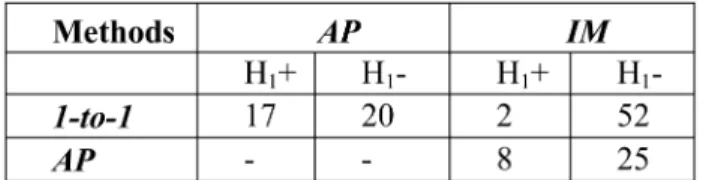
In this section, we compare the best methods out of the three different modeling approaches to predicting customer behavior. As stated in Sections 6.1 and 6.2, we selected the APmethod to represent statistics-based grouping methods because it outperformedHCandEC, and theIMmethod to represent direct grouping methods because it outperformed IGandIR. As a result, we compareAP,IM, andone-to-one methods across the six data sets, three dependent variables per data set, two classifiers, and three performance measures. This resulted in a total of 108 Mann-Whitney tests per a pairwise comparison.

Table 4 summarizes the three pairwise comparisons by listing the number of statistical tests rejecting the null hypothesis (I) at 95 percent significance level. As is evident

4. Methods A (as indicated in the hypotheses H0, H1þ, and H1

described above) are listed in the rows, and methods B from the aforementioned hypotheses are listed in the columns of this and other tables presented in this section (Tables 2, 3, 4, 5, and 6).

TABLE 2

Performance Tests across All Statistics-Based Segmentation Methods for Hypothesis Test (I)

Numbers in columns H1þ andH1-indicate the number of statistical

tests that reject hypothesisH0. Total significance tests per method to

method comparison pair is 108.

TABLE 3

Performance Tests across All Direct Grouping Methods for Hypothesis Test (I)

Numbers in columnsH1þ andH1-indicate the number of statistical

tests that reject hypothesisH0. Total significance tests per method to

method comparison pair is 18.

TABLE 4

Performance Tests acrossOne-to-One,AP,

andIMfor Hypothesis Test (I)

Numbers in columnsH1þ andH1-indicate the number of statistical

tests that reject hypothesisH0. Total significance tests per method to

from the number of statistically significant test counts, IM clearly dominates one-to-one, which in turn slightly dom-inatesAP.

As Tables 5 and 6 show, whileone-to-onedominatesAPfor high-volume customers,APslightly dominatesone-to-onefor low-volume customers, thus reconfirming results demon-strated in [21] where modeling customers in segments using good clustering methods and low-volume transactions tend to perform better than modeling customers individually. We also note that one-to-oneperforms somewhat better against IM among high-volume data sets relative to low-volume data sets, which does make sense as the high-volume customers are more likely to have enough transaction data to effectively model individual customers. However,IMstill shows significant performance dominance over one-to-one and AP across all the experimental conditions, including high- and low-volume customers.

To get a sense of the magnitude of the dominance thatIM has overone-to-one, we computed the difference between the medians of each distribution. For a particular data set, dependent variable, classifier, and performance measure, we took the two distributions of the performance measures across all the segments for the IM and all the individual customers for theone-to-onemethods. Then, we determined the medians of the two distributions5_{(one forIMand one}

forone-to-one) and computed the differences between them. We repeated this process for all the 108 comparisons across the six data sets, three dependent variables per data set, two classifiers, and three performance measures, and plotted out the histograms of the median differences for the CCI, RME, and RAE measures in Figs. 4a, 4b, and 4c, respectively. Note that to plot out histograms across real values, we grouped the median differences across the distribution comparisons into bins along the x-axis, while the y-axis represent the number of tests that falls within the median difference bin. The negative values for the CCI measure and positive values for the RME and RAE measures in Figs. 4a, 4b, and 4c show thatIMsignificantly outperforms theone-to-onemethod across most of the experimental conditions, thus providing additional visual evidence and the quantitative extent of the dominance ofIMoverone-to-onethat was already statistically demonstrated with the Mann-Whitney tests.

We also did the same type of comparison for theAPand the IM methods. In Figs. 5a, 5b, and 5c, we show the left

skewed median difference distribution for the CCI measure and the right skewed median difference distributions for the RME and RAE measures. As in the case of IMversus one-to-one, Figs. 5a, 5b, and 5c clearly demonstrate IM’s dominance overAP.

Last, we did the same type of comparison for theAPand the one-to-one methods, and the results are reported in Figs. 6a, 6b, and 6c. As Fig. 6a shows,one-to-onedominates AP in terms of median CCI difference distributions. However, the small difference in RME error and the relatively evenly distributed RAE median difference dis-tribution indicate that one-to-one produces approximately the same amount of errors asAP. Thus, unlike the case of IM’s dominance overAP, theone-to-oneapproach does not clearly dominateAPacross all the experimental conditions.

6.4 Performance Distributions of the One-to-One, AP, and IM Methods

We can gain further insight into the issue of performance dominance by plotting percent histograms of CCI distribu-tions across different methods and different experimental conditions. Because of the space limitation, we present only three representative examples of these 108 performance measure histograms in Figs. 7a, 7b, and 7c.

Fig. 7a shows the histogram of the CCI performance measure distribution of the Naı¨ve Bayes models generated by theone-to-one approach across 2,230 unique customer’s data from the high-volume ComScore data set. Thex-axis indicates the actual CCI score from a specific Naı¨ve Bayes model trained and tested on specific customers, while the y-axis indicates the percentage of all the models having the corresponding CCI performance measure. Note that CCI scores vary from 10 percent to 100 percent, and the mean of the distribution is slightly above 50 percent.

Fig. 7b displays the histogram of the CCI performance measure distribution of the Naı¨ve Bayes models generated by theAPsegmentation method. Note how the CCI scores now have a tighter range, from close to 20 percent to 60 percent correct if we discount some outliers. However, the mean of the CCI distribution is significantly lower, at a little less than 40 percent. This illustrates our findings in the previous section where, compared to one-to-one, AP has reduced variance and error but also has a lower CCI measure. This finding is consistent with the results of the Mann-Whitney distribution comparison tests for one-to-one versus AP, as reported in Table 4.

Fig. 7c shows CCI distribution generated by the IM methods. Note that the distribution is slightly wider than

TABLE 5

Performance Tests acrossOne-to-One, AP, andIMfor

Hypothesis Test (I) among High-Volume Customers

Numbers in columns H1þ andH1-indicate the number of statistical

tests that reject hypothesisH0. Total significance tests per method to

method comparison pair is 54.

TABLE 6

Performance Tests acrossOne-to-One,AP, andIMfor

Hypothesis Test (I) among Low-Volume Customers

Numbers in columnsH1þ andH1-indicate the number of statistical

tests that reject hypothesisH0. Total significance tests per method to

method comparison pair is 54.

5. We selected the medians, rather than the means, of these performance measure distributions because these distributions tend to be highly skewed and the medians are more representative of the performance of the distributions than their averages.

Fig. 4. Median difference distributions ofone-to-oneversusIM.

Fig. 5. Median difference distributions ofAPversusIM.

Fig. 6. Median difference distributions ofone-to-oneversusAP.

Fig. 7. Sample histograms of CCI measures generated by theone-to-one,AP, andIMmethods using Naı¨ve Bayes on the attribute “day of the week” for high-volume ComScore data.

that ofAP, ranging from 30 percent to 90 percent. However, IMhas tighter variance thanone-to-oneand does not drop in CCI mean relative toone-to-oneand definitely has a higher mean compared toAP. This CCI distribution generated by IM clearly shows improved performance over theAP and one-to-one methods for the reasons demonstrated above, which is consistent with the results of the Mann-Whitney comparison tests as also reported in Table 4.

Again, Figs. 7a, 7b, and 7c provide only three examples of distributions of the CCI measure out of the total of 108 histograms. However, these examples are very typical and clearly delineate the differences between theIM,AP, and one-to-onemethods. Therefore, these selected CCI histograms provide additional insights into the nature of the IM dominance over theone-to-oneandAPmethods, as demon-strated in Tables 4, 5, and 6 and Figs. 4a, 4b, 4c, 5a, 5b, and 5c. In summary, our empirical analysis clearly shows that, contrary to the popular belief [37], theone-to-oneapproach is definitely not the best solution for predicting customer behaviors. On the other hand, IM, which is essentially a microsegmentation approach to segmentation, shows clear dominance over all methods tried in our experimental settings.

However, we noted that there are some high performing size-one segments that were present in the distribution of one-to-oneCCI in Fig. 7a, which did not get picked by theIM method as presented in Fig. 7c. This shows that, while the IMmethod is statistically dominant overone-to-oneandAP, IM is stillnotthe optimal segmentation solution described in Section 2. Nevertheless, IM’s dominance over other popular segmentation methods across all the experimental settings indicates that it constitutes a reasonable approach toward reaching the final goal of generating best compu-tationally tractable approximate solutions of the intractable optimal segmentation problem.

7

I

N

D

EPTH

A

NALYSIS OF

IM

In this section, we make a closer examination of the segments created by the IMmethod. Specifically, we want to study the distribution of segment sizes generated byIM and investigate ways to improveIM.

Fig. 8 shows the distribution of segment sizes generated by IMfor the high-volume customer data sets aggregated

over all the experimental conditions. We note that the overall counts of segments peak at segments of size two and then decrease steadily as the segment sizes increase. We also observe small counts among segments of odd sizes, which is an expected artifact of the IM algorithm where segment groups of roughly equal sizes were iteratively merged to improve performance. However, IM does not inherently discriminate against segments of size one. Rather, segments will remain as size one if there are no other segment, once combined, that could improve the new combinations’ overall fitness. Thus, these observations provide evidence against theone-to-oneapproach to personalization, as most of size-one segments do find at least one other size-one segment to merge and improve the overall performance, as evident from the spike in size-two segments in Fig. 8.

Fig. 9 shows the distribution of segment sizes generated byIMacross low-volume customer data sets. Interestingly, the spike of the segment size distribution occurs at segments of size four. This does make intuitive sense, as low-volume customers need to form bigger groups in order to reach the “critical mass” in terms of the data necessary for building good predictive models. Taken together, both Figs. 8 and 9 suggest that IM’s dominance over one-to-one andAPis largely due to the formation of large numbers of small customer segments, thus adding support to the use of microsegmentation in forming robust and effective models of customer behavior.

The distribution of segment sizes generated by IM (as shown in Figs. 8 and 9) clearly indicates thatIMwas able to find better performing groupings than just simple size-one segments. The peak at segment sizes of two and four forIM implies that segments of small sizes are better performing segments that significantly outperform their respective individual segments of size one, as demonstrated from IM’s dominance overone-to-one.

While the IM direct grouping approach does not con-stitute an optimal grouping, the lack of size-one segments after many rounds of attempted segment merges implies that there will not be many size-one segments in the optimal solution. In addition, the optimal solution will definitely dominate theone-to-onesolution, and we conjecture that it will contain predominantly small-sized segments, resulting in a microsegmented solution, as in the case of IM. We emphasize that this lack of size-one segments in the optimal

Fig. 8. The distribution of segment sizes generated byIMacross high-volume data sets.

Fig. 9. The distribution of segment sizes generated byIMacross low-volume data sets.