econ
stor
www.econstor.eu
Der Open-Access-Publikationsserver der ZBW – Leibniz-Informationszentrum Wirtschaft
The Open Access Publication Server of the ZBW – Leibniz Information Centre for Economics
Nutzungsbedingungen:
Die ZBW räumt Ihnen als Nutzerin/Nutzer das unentgeltliche, räumlich unbeschränkte und zeitlich auf die Dauer des Schutzrechts beschränkte einfache Recht ein, das ausgewählte Werk im Rahmen der unter
→ http://www.econstor.eu/dspace/Nutzungsbedingungen nachzulesenden vollständigen Nutzungsbedingungen zu vervielfältigen, mit denen die Nutzerin/der Nutzer sich durch die erste Nutzung einverstanden erklärt.
Terms of use:
The ZBW grants you, the user, the non-exclusive right to use the selected work free of charge, territorially unrestricted and within the time limit of the term of the property rights according to the terms specified at
→ http://www.econstor.eu/dspace/Nutzungsbedingungen By the first use of the selected work the user agrees and declares to comply with these terms of use.
Weisbrod, Julian; Vollmer, Sebastian; Holzmann, Hajo
Conference Paper
Perspectives on the World Income Distribution:
Beyond Twin Peaks Towards Welfare Conclusions
Proceedings of the German Development Economics Conference, Göttingen 2007 / Verein für Socialpolitik, Research Committee Development Economics, No. 32Provided in cooperation with: Verein für Socialpolitik
Suggested citation: Weisbrod, Julian; Vollmer, Sebastian; Holzmann, Hajo (2007) : Perspectives on the World Income Distribution: Beyond Twin Peaks Towards Welfare Conclusions,
Proceedings of the German Development Economics Conference, Göttingen 2007 / Verein für Socialpolitik, Research Committee Development Economics, No. 32, http:// hdl.handle.net/10419/19885
Perspectives on the World Income Distribution
-Beyond Twin Peaks Towards Welfare Conclusions
Hajo Holzmann
∗Sebastian Vollmer
†Julian Weisbrod
‡Abstract
This paper contributes towards the growing debate concerning the world distribution of in-come and its evolution over that past three to four decades. Our methodological approach is twofold. First, we formally test for the number of modes in a cross-sectional analysis where each country is represented by one observation. We contribute to existing studies with technical improvements of the testing procedure, enabling us to draw new conclusions, and an extension of the time horizon being analyzed. Second, we estimate a global distribution of income from national log-normal distributions of income, as well as a global distribu-tion of log-income as a mixture of nadistribu-tional normal distribudistribu-tions of log-income. From this distribution we obtain measures for global inequality and poverty as well as global growth incidence curves.
JEL classification: O0, C5, I3, F0
Keywords: Convergence, Silverman’s test, non-parametric statistics, bimodal, global income distribution, poverty, inequality, growth incidence curves.
Acknowledgements We would like to thank Stephan Klasen and Stefan Sperlich for their helpful comments and suggestions. Hajo Holzmann acknowledges support from the Deutsche Forschungsgemeinschaft, Grant MU 1230/8-1. Sebastian Vollmer acknowledges support from the Center for Statistics, Goettingen.
∗Institute for Mathematical Stochastics, Georg-August-University Goettingen
†Ibero-America Institute for Economic Research and Institute for Statistics and Econometrics, Georg-August-University Goettingen. Corresponding author: Platz der Goettinger Sieben 3, 37073 Goettingen, Germany. Sebastian.Vollmer@wiwi.uni-goettingen.de
1
Introduction
Since the early 1990s a renewed interest in cross-country income convergence has been moti-vated by a growing literature concerning growth theory and growth empirics as well as general economic welfare questions. Two main questions are the centre of this debate. Firstly, in how far could the observed change of the income distribution and possible cross-country convergence either support or refute the neo-classical growth model, which, given its assumptions, would im-ply some type of conditional1 β-convergence across economies. Alternatively, in how far could
the change in world cross-country income distribution support the strand of new growth the-ories in economics? Secondly, could the change in cross-country income distribution offer any insight into the ranking and relative income differences of economies and thus make suggestions concerning global welfare and income inequality. Obviously, a divergence of cross-country per capita income toward two different peaks would suggest the existence of multiple equilibria for different national economies and thus a poverty trap for the world’s poor nations. This would call for intervention through economic policy possibly adjusting the parameters of respective growth models such that the observed diverging trend could be reversed.
However, as others before, we strongly caution to assume that a divergence within the cross-national income distribution is automatically equal to a divergence of the global income distribution and/or global welfare deterioration. Clearly, it has certain advantages to analyse the behavior of average national per capita income as the unit under scrutiny, the national economy, is a major policy maker in particular with regards toward economic growth models. Hence, if national income growth is the key to welfare improvement it is important to understand the factors hampering or fostering growth, which might be studied best by comparing national economic performances. However, in order to consider global welfare, the actual global income distribution should be of more concern than the cross-country per capita income comparison. Thus, in this paper we distinguish between three different types of distributions. Firstly, the classic cross-country or cross-national income distribution in which every country is treated as a single observation. Secondly, a weighted cross-national distribution in which national income averages are weighted by the countries population share. Lastly, we calculate a mixed-lognormal 1 Conditional on the parameters of the extended Solow model governing the countries under inspection. Thus,
the neo-classical growth model is not contradicting a twin peak convergence club phenomenon as such. This is due to the fact, that if two groups of countries are governed by different parameters, but display within group homogeneity of parameters, it would imply a divergence of the two groups, but a within group convergence of economies to their respective group steady state.
global income distribution, which gives an estimate of the income distribution for all the world’s citizens.
This paper contributes to the existing debate in two ways. Firstly, it places the existing literature on a sounder empirical footing by proving econometrically that the cross-national per capita income distribution does indeed display and tend to an ever stronger bimodal or even multimodal distribution. In order to prove this, we apply a nonparametric method -the Silverman test - using boundary kernels which accounts for -the non-negativity of income data of the cross-country income distribution. This allows a sound econometric test for the existence of uni- vs. bimodal or even multimodal distributions, which cannot be strictly inferred from visual inspection or cross-country regressions alone. Furthermore, the Silverman test is not only applicable to the economic questions stated above, but a useful econometric tool for various economic questions that have the behavior of a distribution at heart. Secondly, and more importantly, it introduces an alternative approach of a mixed log-normal distribution to model a world income distribution which allows us to answer fundamental global welfare questions. Hence, utilising this global income distribution we report the evolution of global income inequality and poverty, applying various standard measures. Furthermore, we construct global growth incidence curves that indicate which semi-decades experience the highest rates of pro-poor growth. Moreover, we compare our results with existing studies concerning global income distribution (in particular Sala-i-Martin, 2006) to support or refute their conclusion.
The paper is structured as followed: Section 2 will discuss the methodology of the Silver-mann test and, following Bianchi (1997), we derive results for the classic cross-national income distribution approach. Furthermore, we estimate in Section 3 the world-income distribution as a mixture of the respective national income distributions, where the weights of the mixture are determined by the proportion of the nations population relative to the world population. The national income distributions are modeled parametrically by a log-normal distribution, where the parameters of the log-normal distribution can be determined form the real PPP GDP/per capita and the Gini of the respective country. The resulting estimate of the world income dis-tribution allows to obtain conclusions regarding global income inequality, poverty and rates of pro-poor growth.
2
The Classic Cross-National Income Distribution:
Revisiting the Twin Peaks Debate
2.1
Introduction
The convergence hypothesis states that poorer economies are growing faster than richer ones, hence, catching up such that eventually there will be no differences between real average per capita income across countries. This would imply a unimodal cross-national distribution of income2 which should become constantly less dispersed. The literature distinguishes between
two types of convergenceβ-convergence andσ-convergence (Sala-i-Martin 1996). By definition β-convergence occurs, if the coefficient on initial income is negative when regressed on the change of log real income, or in words, if initially poorer economies grow on average faster than the initially rich. Moreover, σ-convergence is defined as the decrease of the dispersion of the entire income distribution. If there are no other control variables in the growth regression, we speak of absolute β-convergence, which would be a necessary but not sufficient condition for σ-convergence. Not sufficient due to the fact that due to rank switching β-convergence can be shown, whilst the dispersion of the income distribution remains unaltered. Thus, for the convergence hypothesis to hold we need absolute ß-convergence and σ-convergence such that the income distribution converges to one common mode.
In the empirical growth regression literature, which is based on the neo-classical growth model (Mankiw, Romer & Weil 1992, Barro 1991, and many more), the initial income term is always significantly negative in cross-country growth regressions, as long as certain other basic parameters of the neo-classical growth model are controlled for. Hence, we find consistent and very robust conditional β-convergence in a wide array of growth regression specification. However, conditionalβ-convergence by no means implies a unimodal convergence of the income distribution, as conditionalβ-convergence only shows that, given certain parameters controlling for each countries steady state, countries further from their steady state undergo faster growth due to transitory dynamics. Thus, a twin peak or in fact multimodal income distribution is theoretically no contradiction to the neo-classical growth model (Mankiw, Romer & Weil, 1992, Gailor, 1996)3. Only if all parameters of the extended Solow growth model (including technology
2 All income data is real per capita GDP PPP as reported in Summer, Heston and Aten (Penn World Tables
6.2)
and human capital) would be homogenous globally we would expect absoluteβ-convergence and σ-convergence to occur and the lack thereof to refute the neo-classical growth model. Hence, new growth theories such as the AK or the Romer model (Romer, 1991) which are, due to the lack of marginal returns, in theory applicable to all conceivable income distributions cannot be shown to be superior on the grounds of a lack of unimodal behaviour of the income distribution4.
Furthermore, other models (for example Bernard & Jones, 1996) help to reconcile this debate by explaining the existing convergence pattern via the behavior of technological change. Thus, the cross-national convergence debate as proof for either strain of economic growth theory is misguided.
However, the behaviour of the cross-national income distribution is for many other reasons of great interest. In particular, the development of twin peaks would characterise a world of growing cross-country average income polarization and suggest the existence of multiple equilibria, which would call for policy intervention. Numerous papers (Jones, 1997; Quah, 1996a, b; Sala-i-Martin, 1996) have this debate at heart and discuss which type of convergence governs the development of the cross-national income distribution and what is to be expected in the future. In particular, they show that a focus onβ-convergence is informative on the nature of intra-distributional dynamics but cannot convey information concerning the development of the entire distribution, which appears to be polarizing. In order to overcome this traditional shortcoming of the β-convergence debate, probabilistic income mobility models are used to estimate likelihoods of convergence groups. Hence, debating whether the twin peak phenomena is persistent as probabilities are too low (Quah, 1996a,b) or only a temporary occurrence due to increasing frequencies of growth miracles (Jones, 1997)5. Our test results contribute to the
overall debate by statistically demonstrating the emergence of twin peaks in the cross-national income distribution.
2.2
Testing for Twin Peaks: Methodology & Data
Following most other papers our analysis is based on income data from the Penn World Tables Version 6.2 (Summer, Heston & Aten, 2006), from which we extract the real PPP GDP/per capita and the population series for all years and countries available. In order to compare our
parameters of the production function, but it has been shown elsewhere (Mankiw, Romer & Weil, 1992; O Galor, 1996) that the obtained results are in principal conceivable with the stylized fact
4 despite all other merits they might posses
observations over time, we restrict ourselves to those countries having complete income data for the whole time period considered. This restriction leaves 93 countries for the period from 1960 to 2003 and 127 countries for the period 1970 to 2003 in our analysis. In the second case these countries represent about 90 percent of the world´s population.
A simple way to look at the world income distribution is a cross-sectional analysis where each country is represented by one observation. Kernel density estimates are widely used to get an impression of the underlying distribution in such or similar cases. Suppose thatx1, . . . , xn
are independent observations with density f. The kernel density estimator for the densityf is defined by ˆ f(x;h) = (nh)−1 n X i=1 K µ xi−x h ¶ ,
whereh >0 is a smoothing parameter, called the bandwidth, andKis a kernel function which integrates to one. The features of the resulting estimate ˆf(x;h) such as peaks and valleys strongly depend on the choice of the bandwidth and to a lesser extend on the choice of the kernel functionK.
Silverman (1981) observed that the number of modes (i.e. of local maxima) of ˆf(x;h) is a monotonically decreasing and right-continuous function of the bandwidth, if one uses the stan-dard normal density as kernel functionK. He used this fact to define thek-critical bandwidth hc(k) as the smallest bandwidth such that ˆf(x;h) still has kmodes, and not yetk+ 1 modes.
Intuitively speaking, if thek-critical bandwidthhc(k) is large, a lot of smoothing is required so
that the density estimate ˆf(x;h) only has k modes. This indicates that the target density f might have more than k modes. In order to put this observation into a statistical test and to assess its significance, Silverman (1981) suggested to use the so-called smooth bootstrap, details of this method can be found in Silverman (1981), Fisher et al. (1994) or Bianchi (1997).
Bianchi (1997) first applied Silverman’s (1981) test to the world distribution of real PPP GDP/per capita. We shall do a similar analysis here, over the extended time-horizon up to 2003 for both the PPP GDP/per capita itself as well as for its logarithm. Furthermore, we take into account some technical modifications and extensions. In fact, it is well known that the critical value of the Silverman test, based on the smooth bootstrap, is conservative. Thus, if one tests the hypothesisHk that the densityf has at mostkmodes against the alternative that it
has more than kmodes with a nominal level α, the actual level of the test will be quite below α. Hence, one does not reject the hypothesisHk often enough. For testing the hypothesisH1
of single mode against more than one mode, Hall and York (2001) suggested a calibration of the critical value so that the test actually achieves its nominal level. We used their calibration method in this (most important) testing situation. Furthermore, the PPP GDP/per capita is evidently a non-negative quantity, and it has a strong mode near zero. In order to avoid the bias problem near zero (cf. Wand and Jones, 1995), for the original PPP GDP/per capita data we use a renormalized version of the Gaussian kernel (boundary kernel) near zero. As shown in Fig. 1 and in contrast to Figs. 1 and 5 in Bianchi (1997), taking into account the boundary affect makes the strong mode near zero much wider.
At this point, it has to be stress that the number of modes of the original income does not neccessarily have to be equal to the number of modes of the logarithmized distribution. This is because the density g of the logxi is g(t) = f(et)et. Taking the derivative, one sees that
the derivativeg0 will possibly have a different number of zeros than f0, and thus g will have a
distinct number of modes. If one is interested in the number of modes on a linear scale, one should use the original income data but if one wants to investigate modes on an exponential scale, one should use their logarithm.
2.3
Results of Silverman’s test
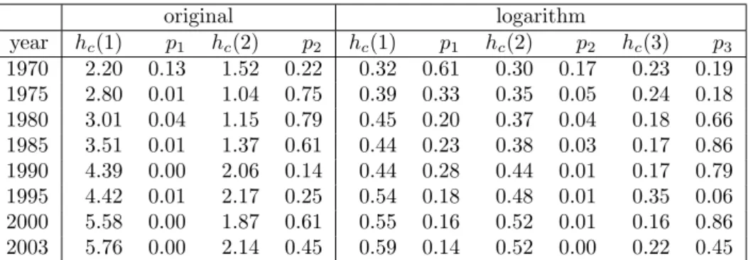
Our analysis for the period 1970 to 2003 supports the findings of Bianchi (1997) for 1970 to 1989 and carries them onward until 2003. In table 2 we give the results of the tests starting in 1970 in 5 year steps and including 2003. While the hypothesis of one against more modes cannot be rejected in 1970 at a 5% level, it can be rejected for all consecutive years. Furthermore, it can be observed that the corresponding p-values have a tendency to decrease, increasing the statistical significance of the second mode. The hypotheses of two against more modes can never be rejected, confirming the bimodal structure of the density. The test results of the years 1960 to 2003, based on a smaller number of countries, are displayed in table 1. The results correspond to those for the larger sample. In 1960-1970, the hypothesis of one mode cannot be rejected at 5%, afterwards, it is always rejected in favour of two modes.
For the log-income data the results differ. As shown in tables 1 and 2, the hypothesis of one mode cannot be rejected for any year at a 5% level. However, the p-values decrease strongly over the years up to 2003. Moreover, starting from 1980 the hypothesisH2that the density has
glance somewhat counterintuitive. The interpretation is that there is statistical evidence that the density is not bimodal, it is either unimodal or it has three modes. Since the p-values for H1 (and alsoH2) decrease over time, while the p-value forH3(three modes) strongly increases,
we expect that the log-income density evolves toward three, not too significant modes. This is also reflected in Fig. 2. The optimal bandwidth gives a density estimate with three modes in 2003, all of which, however, are not too significant. In fact, the distance between this “optimal” density estimate and the density estimate based onhc(1) is not very large, either. To conclude,
the log-income distribution appears to evolve from a unimodal density in 1970 toward a density with three modes in 2003, which is, however, still close in shape to a unimodal density, i.e. its additional modes are not very distinctive.
We conclude that our findings cannot be reconciled with the absolute convergence hypothesis. However, this does not imply a contradiction to the concept of conditional convergence or the neo-classical growth model. Nevertheless, the twin peak divergence indicates, if one asumes the neo-classical as true, that some poorer countries are stuck in a poverty traps as long as a number of structural conditions do not improve.
3
The global income distribution and welfare implications
3.1
Approaches toward a population weighted cross-national or global
income distribution
The classical cross-national income comparison approach suffers from severe shortcomings if one wishes to draw conclusions concerning global welfare, inequality or poverty. The major problem of the simple cross-sectional approach is the fact that the observation of Luxemburg counts as much as the observations of, for example, China or India. Therefore, the average welfare of a Luxembourgian is weighted much higher than the welfare of the average Chinese. Thus, more recently a number of papers have shifted the debate away from the classical cross-national income distribution approach towards a global income convergence analysis. Two main approaches have been utilized. The first group of papers is based on the classical cross-national income distribution but where the observations are weighted by the nations’ respective population (Theil, 1979; Berry, Bourguignon and Morrisson, 1983; Theil & Seale, 1994; Schultz, 1998; Firebaugh, 1999; Melchior, Telle & Wiig, 2000).
Unfortunately, there is no well defined way of how to weight the observations. The number of modes and the whole structure of the distribution in fact changes when different weights are used. This is due to the fact that the concentration which is given to each observation is only well determined relative to the weight given to other observations but not in absolute terms. In other words, by variation of the absolute concentration one can more or less create any number of modes one wishes. Thus, this method allows for the comparison of weighted means, but is not well suited for the estimation of a global income distribution.
The second group of papers model the global income distribution, or a distribution limited to major economic players, by taking into account the underlying national income distributions (Dowrick & Akmal, 2005; Bourguignon & Morrisson, 2002; Quah 2002; Sala-i-Martin, 2002a, 2006). In fact, an objective way to construct the global income distribution from the distinct national income distributions is as a population weighted finite mixture of the national income distributions. Intuitively, if one picks at random an individual with a certain income from this global income distribution, one first randomly draws the country its belongs to (with probability equal to that countries proportion in the world population), and then obtains its income from the corresponding country income distribution.
The problem in this approach is hence to determine the national income distributions. Sala-i-Martin (2006) argues that from the methodological point of view, one should use nonparametric kernel estimates instead of parametric models for the country income distributions, since these do not assume any specific shape for the income distributions. While we agree with it on the methodological basis, in our opinion nonparametric modelling would require actual income data of all required countries, and on a comparable basis. Sala-i-Martin (2006) uses national accounts and survey data for the estimation process. However, these are only available for some of the relevant countries (groups A and B of his analysis), and even they are not really comparable. Because of this lack of relevant data, we prefer to model the national income distributions parametrically as log-normally distributed.6 The relevant parameters of each countrie’s
log-normal income distribution can be readily determined from its real PPP GDP/per capita and its Gini coefficient (cf. Section 3.2). Hence, the amount of data required for this approach is far less than for non-parametric estimation of the country distributions. Even though the log-normal 6 After this work was completed, we became aware of a preprint cited in Sala-i-Martin (2006), ” The world
distribution of income estimated from log-normal country distributions”, Sala-i-Martin, 2004, in which he seems to use a similar approach. We were however not able to obtain this paper.
distribution may not be a completely adequate model for each countrie’s income distribution, the effect will be small on the final world income distribution obtained as a population-weighted mixture. In addition to requiring less and more readily available data, our approach also has some methodological merits. In particular, the resulting global income distribution (a finite mixture of log-normal distributions) is much easier to handle than a non-parametric analogue, and it is e.g. easy to sample from this distribution. We will exploit this advantage to construct growth incidence curves of the world income distribution for several years.
3.2
Methodology & Data
As stated in Section 3.1, the national income distributions will be modelled by using a log-normal distribution. Formally, the log-normal distribution LN(µ, σ) is defined as the distribution of the random variableY = exp(X), whereX ∼N(µ, σ) has a normal distribution with meanµ and standard deviationσ. It can be shown that the density ofLN(µ, σ) is
f(x;µ, σ) = 1 xσ√2π·e
−(log(x)−µi)2/2σ2
, x >0,
and its mean and variance are given respectively by
E(Y) = eµ+σ2/2
,
V ar(Y) = (eσ2−1)e2µ+σ2. (1)
We should briefly discuss discuss the interpretation of the parametersµandσ, which is different from that for the normal distribution. In fact, from (1) one sees that logµis proportional to the expectation and (logµ)2is proportional to the variance, and in fact, logµis the scale parameter
of the log-normal distribution, whereasσis a shape parameter. Since the Gini coefficient should be invariant under changes of scale (it should not matter whether income is measured in Euro or in dollar), it should be independent ofµand only depend onσ. This is indeed the case: The Gini coefficientGofLN(µ, σ) is given by
where Φ is the distribution function of the standard normal distribution. Therefore, the para-meters µand σof LN(µ, σ) can be determined from the mean EY and the Gini coefficient G as follows. σ = √2 Φ−1 µ G+ 1 2 ¶ , µ = log(E(Y))−σ2/2.
In summary, the parametersµandσof each countrie’s log-normal income distribution are easily determined from the real PPP GDP / per capita (EY) and its GiniG. While these data are much more readily available than the whole income data of the countries, the coverage of inequality measures, such as the Gini, does not start in earnest until the late 1970s or even 1980s. The biggest inequality database available is the UNU WIDER dataset, which reports all available Gini measures of inequality with additional information concerning area covered and base data utilised. Due to different methodology, the reported Ginis are not fully comparable over time and countries. However, Gr¨un and Klasen (2006) carefully constructed a more consistent Gini dataset based on WIDER raw data. Hence, we utilize their much improved dataset 7 as our
basic inequality data set. Furthermore, as inequality does not change too dramatically over time, we assum that the first real observation of the Gini in any given country to be equal to its initial (1950) level of inequality. Starting from this initial level we used a moving average to catch changes in trends of inequality for the periods for which our data coverage was extensive, mostly past the 1970s.
To conclude this section, we formalise how the density of the world income distribution fW
is obtained as a mixture of national (log-normal) distributions. Assuming that there are n countries under investigation and that the (log-normal) density of the distribution of countryi is given byf(x;µi, σi). Then fW(x;µ1, . . . , µn, σ1, . . . , σn, p1, . . . , pn) = n X i=1 pif(x;µi, σi),
where pi is equal to the proportion of countryi´s population in the whole population of these
ncountries. It has to be stressed that although the densityfW is a simple finite mixture of the
component country densitiesf(x;µi, σi), this does not transfer to relevant quantities such as the
Gini or other inequality or poverty measures: the world GiniGW is not simply the corresponding
finite mixture of the country GinisGi. Nevertheless, once the parameters of the densityfW are
estimated, it is not difficult to estimate all relevant inequality and poverty measures by Monte Carlo simulation fromfW. To this end we used a random sample fromfW of size 105. Finally,
let us remark that if the world incomeY is distributed asfW, than the log world income logY
has density lfW(x;µ1, . . . , µn, σ1, . . . , σn, p1, . . . , pn) = n X i=1 piφ(x;µi, σi),
where φ(x;µ, σ) is the density of the N(µ, σ) Thus lfW is simply a finite mixture of normal
densities.
3.3
Convergence, Global Inequality and Poverty
Figures 3 and 4 show estimates of the global income distribution as well as of the log-income distribution, determined as discussed in Section 3.2, for selected years. Two things are apparent at a first glance. Firstly, the average global income increased dramatically over the given time period. Secondly, the global world income distribution has become less dispersed over time. Interestingly, the 1970s still seem to display a twin peak phenomenon in the global log-income distribution, however, these twin peaks disappear over the years and in particular between 1990 and 2003. Thus, the results show clearly global income expansion and convergence of real global individual income in $US (PPP). One hypothesis might be that the increased globalisation of the time period lead to a further integration of the world citizens’ income. The inequality measures reported in Table 4 confirm this first impression as all measures decline over time. In particular, a persistent decline of global income inequality can be observed past the mid1970s, as can be seen in Graph 7. This date roughly corresponds to a relative income growth loss in the West due to the oil price shocks and a simultaneous increased income catch-up of mainly, but not exclusively, the South East Asian Tigers, followed by China and later India.8 Thus,
the median global citizen did not only get richer over the given time period, but additionally his or her relative income position as compared to the top 5 percentiles of the global income distribution improved considerably. This pattern becomes even more apparent if one considers what happened to poverty and percentile specific growth.
An estimation of global poverty is inherently tricky and controversial due to multiple method-8 A paper concerning regional decomposition of the above results is in preparation.
ological shortcomings. All poverty lines are in many ways arbitrary as they depend on re-searchers’ choices of what is poor and how this definition is compared across space and time.9
Nevertheless, a poverty line is useful as it allows researchers to use a bench mark and track poverty changes over time and space given the definition of poverty. The best known and most cited poverty line is the $1 or $2 (PPP, 1993) per day poverty line developed by the World Bank. This poverty line is supposed to be the monetary minimum to cover basic needs and is to be used as an expenditure poverty line in household surveys. Ravallion (2004)10 has argued
that the expenditure poverty line should be roughly half of an income poverty line, thus our $2 US (PPP) applied to income should be roughly comparable to the World Bank’s $1US (PPP) poverty line applied to expenditure data. 11 In the end we decided to stick to the World Banks
definition as it allows our results to be comparable to other results by Chen and Ravallion (2004) and Sala-i-Martin (2006). Furthermore, we show in figure 6 that any reasonably selected poverty line would show a decline in the poverty headcount ratio as the cumulative distribution func-tion of global income of subsequent time periods are dominant over the cumulative distribufunc-tion function of the prior time period. Our poverty line is set at $469.9 US (PPP) and $935.45 US (PPP) a year, which corresponds to the World Bank 1993 poverty line of $1.08 US and $2.15 US per day adjusted to our income baseline year 2000 respectively. 12
Table 3 below shows the results for the Foster-Greer-Thorbecke (FGT) poverty measures
FGT:Pα= 1 N q X i=1 ((z−yi)/z)α
for the poverty headcount (α=0), poverty gap ratio (α=1) and the squared poverty gap (α=2) (should include the poverty gap squared). The results are reported for our $1 and $2 a day poverty line respectively. Furthermore, the absolute number of people below the two poverty lines is reported. It is apparent that from 1970 to 2003 all measures of poverty, absolute and relative, declined strongly. The percentage of the world population living below $1 a day declined drastically from 22 percent in 1970 to 5 percent in 2003. The reduction of this measure of extreme poverty was particularly rapid in the 1970s and early 1980s as the headcount ratio 9 Reddy and Pogge 2005
10 The Economist 2004.
11 However, it is beyond the scope of this paper to discuss the advantages or disadvantages of certain poverty
lines.
12 adjusted to our 2000 base year $1.08 (1993) per day = $ 1.287 (2000) per day = $469.9 per year. In the
dropped from 22 percent in 1970 to 8 percent in 1984 which corresponds to a decline of the absolute number of people living with less than $469.9 (PPP, 2000) per year from slightly over 800 million in 1970 to roughly 380 million in 1984. From 1984 to 2003 the headcount fell further to 5 percent which corresponds to about 315 million people living below $469.9 (PPP, 2000) per year. Moreover, the poverty gap ratio also displays a constant decline over the given time period, hence, not only did the absolute number of people living in extreme poverty fall, but those which remained poor saw their income improved towards the poverty line.
The results for the $2 poverty line follow a very similar pattern. The headcount declined strongly from 45 percent, almost half the world’s population, in 1970 to 14 percent in 2003. The most dramatic decline of the $2 headcount was in the late 1970s and the 1980s from 44 percent in 1975 to 21 percent in 1990. Overall, the absolute number of people who lived below $935.45 (PPP, 2000) per year declined from 1,654 billion in 1970 to 880 million, in 2003. Furthermore, the poverty gap or ”distance” of those people below the poverty line to the poverty line declined also considerably. Thus, all conceivable measures of poverty show a dramatic decline of global poverty in relative and even in absolute terms, although clearly some decades and some regions experienced more pro-poor progress than others.13 In order to gain a better understanding
concerning the behavior of the world income distribution and the semi-decade specific rates of pro-poor growth a look at the subsequent global growth incident curves is highly informative.
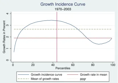
Figures 7 and 8 show global growth incidence curves for different time periods 14. The
main results are summarised in table 5 below. Firstly, if one considers the entire observation period it is apparent that the middle percentiles of the global income distribution experienced the highest growth rates. In fact, the growth rate from the 10th to the 65th percentile of the global population experienced income growth rates above the mean of the growth rates of all percentiles which is equal to 2.67 percent per annum. Thus, the bottom-middle of the global income distribution experienced the fastest income growth which also explains the declining income inequality and global income convergence. This effect is slightly counteracted by the less than average growth performance of the bottom 10 percentiles, with the poorest percentile experiencing the lowest income growth overall. Furthermore, the global average income grew by 1.9 percent per annum, where as the median global individual experienced a 3.3 percent per 13 an analysis of the regional decomposition is in preparation
annum income increase. The rate of pro-poor growth15for the $1 per day poverty line exceeds
with 2.55 percent per annum the growth rate in mean by 0.65 percentage points per annum. Hence, the 34 years from 1970 to 2003 can be termed pro-poor in the relative sense, as the poor experienced higher income growth rates than the average income. For the $2 per day poverty line the period was even more pro-poor as the rate of pro-poor growth with 2.97 percent per annum exceeded the growth rate in mean with even 1.7 percentage points per annum and is even greater than the mean percentile growth rate. Hence, the global growth incidence curves over the period from 1970 to 2003 confirm and strengthen our inequality and poverty results above, as it shows that over the 34 years the income of the poor16has grown much faster than the average
income. In fact, the bottom-middle income percentiles experienced the highest income growth rates explaining global income convergence, declining inequality and falling poverty headcounts. More results from above are confirmed if one looks at decade specific growth incidence curves.
For the first half of the 1970s the top and bottom percentiles of the global income distribution experienced the highest growth rate. If one considers the $1 per day poverty line these years experienced relative pro-poor growth, which is not the case if one applies the $2 per day line, as the bottom-middle of the income distribution experienced only modest growth rates. The second half of the 1970s are characterized by the strongest global growth performance of 2.53 percent per annum in mean income and can be considered poverty neutral if one considers the $1 per day line and relatively pro-poor for the $2 per day definition. It is apparent that the 12th to the 67th percentile had higher growth rates than the average percentile growth rate and thus the bottom-middle of the global income distribution gained the most.
The first half of the 1980s can be considered the most pro-poor over the given time period as the 2nd to 47th percentile experienced very high growth rates compared to the top percentiles. Unsurprisingly, the mean grew by only 1.01 percent per annum, but the rate of pro-poor growth was 5.17 and 5.11 per annum for the $1 and $2 per day poverty line respectively. The second half of the 1980s experiences an increase in the global mean income growth rate to healthy 2.11 percent per annum and is characterized by negative pro-poor growth rates for the extreme poor, at -0.72 percent per annum, and lower than average pro-poor growth rates for the poor, at 1.11 percent per annum. This is mainly due to the fact that even the bottom percentiles from 1st 15 which is the average growth rate of the percentiles below the poverty line as defined by Chen & Ravallion
2003
to 6th experienced an income decline and that overall percentiles, which are considered to be poor under the $1 and $2 per day definition, had been extremely reduced from the previous very pro-poor growth spell. In fact, above mean percentile growth rate was achieved by the 20th to the 67th percentile and for the top 3 percentiles, so the bottom-middle half of the income distribution did catch up further to the upper percentiles. However, the very bottom of the distribution which was still considered poor gained very little. Thus, the 1980s have been the most pro-poor from a global perspective 17. In particular the bottom-middle percentiles grew
consistently closing the income gap between the developing and developed world which can also be seen if one looks at the log-income distribution where the twin peaks start to dissolve over the course of the 1980s. One hypothesis might be that the onset of globalization and export-led growth strategy enabexport-led many global poor to participate in the global growth process in particular in China and South East Asia.
This pattern of global income convergence carries over into the 1990s, as the first five years can be considered relatively pro-poor under the $2 per day poverty line definition, but not under the $1 per day poverty line definition, which comprise only the lowest percentiles. Moreover, the second half of the decade is relatively pro-poor for both poverty lines as the very bottom percentiles experience very high growth rates. The highest growth rates over the decade are achieved by the inter-quartile percentiles that experience above mean percentile growth rates and implies further global income convergence over the 1990s. Hence, at the end of the 1990s no hint of a second peak in the log-income distribution remains. The overall growth rate of mean income follows the previous decade pattern with the first half being characterised by relatively slower growth rates, 1.44 percent, per annum than the second, 2.37 percent.
For the first four years in the new millennium the growth rate of mean income has slowed down again to 1.29 percent per annum. The rate of pro-poor growth is below the average income growth rate with the bottom percentiles growing at only 0.82 percent per annum for the $1 per day poverty line and 0.94 percent for the $2 per day poverty line. The highest growth rates are observed in the upper-middle part of the income distribution.
In the end, our results insinuate that most global poor nowadays live in countries which are most likely stuck in a poverty trap. In other words, even though the global income distribution is converging, due to the tremendous integration of many former developing countries into the 17 even though the 1980s are considered the lost decade in Latin America not that much of the Latin American
”global economy” and a connected income catch-up, it is equally clear that most remaining poor live now in countries which have so far missed out in this process. These are the countries characterized by low average national income which make up the lower mode in the cross-national income distribution and the lowest percentiles in the global income distribution. It is those countries which need to make headway, if one wishes to reduce global poverty further. Moreover, as often reported before, these countries are mainly in Sub-Saharan Africa, in which growth is penalized, as shown in many papers, by lacking institutions, geography or both. A future study will decompose the above results into regional subgroups enabling a confirmation of this hypothesis.
4
Conclusions
To sum up, the results of Silvermann’s test for the classical cross-national income approach clearly proves the emergence of, and ever growing, twin peak phenomenon for the distribution of average national incomes. This implies a polarisation of average national incomes into a rich and a poor convergence club. However, this is per se no contradiction to the neo-classical growth model; it rather indicates that the structural conditions or parameters, which govern these two convergence clubs, differ, such that the countries in the poor convergence club can be argued to be stuck in a low level equilibrium or poverty trap. This realisation would call for policy intervention by the poorer countries and to get the macro-economic framework and growth parameters right to set their countries on a higher and sustainable growth path, which eventually would allow for a catch up with the richer economies.
However, the polarisation of average national incomes does not necessarily imply a divergence of the global income distribution as a whole, as it does not account for the population share of the individual national observation nor the country specific income distribution. Our mixed log-normal approach allows a parametric estimation of the global income distribution, under the assumption of log-normality of the national income distributions and relatively stable national income dispersion as measured by the national Gini coefficient. Our results show that the past 34 years witnessed a strong global income convergence accompanied by a drastic decline of global inequality and poverty no matter what conceivable poverty line is applied. Furthermore, the analysis of growth incidence curves shows that over the past 34 years the 10th to 65th global income percentiles experienced above average percentile growth rates which explains the
occurring global income convergence.
This in itself can be considered a great success as it shows that in particular the bottom-middle global income percentiles managed to catch up to higher levels of income reducing the dispersion of income from a global perspective. On the other hand, the remaining very lowest quintile also experienced he lowest percentile growth rates, such that the remaining extreme poor might be particularly hard to reach. This is likely due to the fact that those remaining poor are mostly citizens of countries whose economies are stuck in a low level income equilibrium and thus fail to connect to the global growth process. However, poverty also remains a pressing issue in many countries which managed to launch their economies on a successful growth tra-jectory, but which have remaining pockets of poverty, in particular in rural areas, within their national boundaries. Thus, any attempt to reduce global poverty even further must focus on those countries stuck in general national poverty traps and on remaining, in particular rural, national pockets of poverty which suffer from very similar structural weaknesses, which hamper their growth potential and disconnect them from the global growth process. The regional de-composition of growth shows that countries and regions which managed to participate the most in globalisation, managed to reduce poverty the fastest, despite considerable caveats of such a process. Thus, integration, under fair conditions, of structural weak economies and pockets of poverty into the global economy should be the best guarantee to reduce global poverty even further assuring that the global community reaches the targeted MDGs.
References
Barro, R. and X. Sala-i-Martin (1992) Convergence. Journal of Political Economy2, 223–251. Bernhard, A. and C. Jones (1996) Technology and Convergence. The Economic Journal 106, 1037–1044.
Berry, A., F. Bourguignon and C. Morrisson(1983) Changes in the World Distribution of Income between 1950 and 1977. The Economic Journal 113, 331–350.
Bianchi, M. (1997) Testing for Convergence: Evidence from Non-Parametric Multimodality Tests. Journal of Applied Econometrics12, 393–409.
Bourguignon, F. and C. Morrisson (2002) Inequality Among World Citizens: 1820-1992. Amer-ican Economic Review92, 727–744.
Bourguignon, F. (2003) The growth elasticitys of poverty reduction: explaining heterogeneity across countries and time periods. In T. Eicher and S. Turnovski, (eds),Inequality and Growth : Theory and Policy ImplicationsMIT Press, Cambridge, Massasuchets.
Datt, G. and M. Ravallion (1992) Growth and Redistribution Components of Changes in Poverty Measure: A Decomposition with Applications to Brazil and India in the 1980s. Jounral of De-velopment Economics38, 275–295.
Dowrick, S. and M. Akmal (2003) Contradicting Trends in Global Income Inequality: A Tale of Two Biases. Review of Income and Wealth51, 201–229.
Durlauf, S. (1996) On the Convergence and Divergence of Growth Rates. The Economic Journal
106, 1016–1018.
Efron, B. (1979) Bootstrap methods - another look at the jack-knife. The Annals of Statistics
7, 1–26.
Firebaugh, G. (1999) Empirics of World Income Inequality. American Journal of Sociology104, 1597–1630.
Fisher, N. I., Mammen, E. and Marron, J. S. (1994) Testing for multimodality. Comput. Statist. Data Anal. 18, 499–512.
1056–1069.
Gruen, C. and S. Klasen (2007) Growth, Inequality, and Well-Being: Comparisons across Space and Time. forthcoming.
Hall, P. and York, M. (2001) On the calibration of Silverman’s test for multimodality. Statist. Sinica11, 515–536.
Heston, A., R. Summers and B. Aten (2006) Penn World Table Version 6.2. Center for Inter-national Comparisons of Production, Income and Prices at the University of Pennsylvania. Jones, C. (1997) On the Evolution of the World Income Distribution. The Journal of Economic Perspectives11, 19–36.
Kremer, M., A. Onatski and J. Stock (2001) Searching for Prosperity. Carnegie-Rochester Con-ference Series on Public Policy 55, 275–303.
Mankiw, G., D. Romer and D. Weil (1992) A Contribution to the Empirics of Economic Growth.
Quarterly Journal of Economics107, 407–437.
Melchior, A., K. Telle and H. Wiig (2000) Globalization and Inequality - World Income Dis-tribution and Living Standards, 1960-1998. Studies on Foreign Policy Issues, Report 6B, Oslo, Norway: Royal Norwegian Ministry of Foreign Affairs.
Quah, D. (1996) Twin Peaks: Growth and Convergence in Models of Distribution Dynamics.
The Economic Journal106, 1045–1055.
Quah, D. (2002) One Third of the World’s Growth and Inequality. CEPR DP3316.
Ravallion, M. and S. Chen (2003) Measuring pro-poor Growth. Economic Letters 78, 93–99. Romer, P.(2002) Endogenous Technological Change. NBER Working Paper3210.
Sala-i-Martin, X. (1996) The Classic Approach to Convergence Analysis. The Economic Journal
106, 1019–1036.
Sala-i-Martin, X. (2002) The Disturbing ”Rise” of Global Income Inequality. NBER Working Paper8904.
Conver-gence, Period. Quarterly Journal of Economics121, 351–397.
Schultz, P.(1998) Inequality and the Distribution of Personal Income in the World: How is it Changing and Why? Journal of Population Economics11, 307–344.
Silverman, B. W. (1981) Using kernel density estimates to investigate multimodality. J. Roy. Statist. Soc. Ser. B43, 97–99.
Theil, H. (1979) World Income Inequality and its Components. Economic Letters2, 99–102. Theil, H. and J. Seale (1994) The Geographic Distribution of World Income, 1950–1990. The EconomistIV, 387–419.
original logarithm year hc(1) p1 hc(2) p2 hc(1) p1 hc(2) p2 hc(3) p3 1960 1.31 0.58 1.01 0.39 0.45 0.17 0.26 0.34 0.19 0.39 1965 1.21 0.92 1.07 0.58 0.39 0.53 0.28 0.29 0.25 0.07 1970 2.39 0.12 1.52 0.29 0.40 0.53 0.34 0.10 0.27 0.03 1975 3.02 0.03 0.96 0.88 0.51 0.17 0.44 0.00 0.19 0.58 1980 3.39 0.03 1.15 0.84 0.45 0.39 0.45 0.01 0.25 0.16 1985 3.95 0.00 1.37 0.60 0.47 0.27 0.42 0.02 0.16 0.89 1990 4.91 0.00 1.63 0.46 0.50 0.27 0.45 0.03 0.19 0.71 1995 4.94 0.01 1.59 0.75 0.56 0.24 0.52 0.01 0.18 0.79 2000 6.07 0.00 1.86 0.70 0.60 0.15 0.54 0.00 0.16 0.83 2003 6.29 0.01 2.14 0.53 0.63 0.11 0.51 0.01 0.16 0.88
Table 1: Silverman results 1960-2003, 93 countries
original logarithm year hc(1) p1 hc(2) p2 hc(1) p1 hc(2) p2 hc(3) p3 1970 2.20 0.13 1.52 0.22 0.32 0.61 0.30 0.17 0.23 0.19 1975 2.80 0.01 1.04 0.75 0.39 0.33 0.35 0.05 0.24 0.18 1980 3.01 0.04 1.15 0.79 0.45 0.20 0.37 0.04 0.18 0.66 1985 3.51 0.01 1.37 0.61 0.44 0.23 0.38 0.03 0.17 0.86 1990 4.39 0.00 2.06 0.14 0.44 0.28 0.44 0.01 0.17 0.79 1995 4.42 0.01 2.17 0.25 0.54 0.18 0.48 0.01 0.35 0.06 2000 5.58 0.00 1.87 0.61 0.55 0.16 0.52 0.01 0.16 0.86 2003 5.76 0.00 2.14 0.45 0.59 0.14 0.52 0.00 0.22 0.45
1970 0 0.05 0.1 0.15 0.2 0 5 10 15 20 25 1980 0 0.05 0.1 0.15 0 5 10 15 20 25 30 1990 0 0.05 0.1 0.15 0 5 10 15 20 25 30 35 2003 0 0.05 0.1 0.15 0 5 10 15 20 25 30 35
Figure 1: Density estimates of the cross country income distributions for the years 1970, 1980, 1990 and 2003 with different bandwidths: L2-optimal bandwidth (solid lines), hc(1) (dashed
1970 0 0.1 0.2 0.3 0.4 4 5 6 7 8 9 10 11 1980 0 0.1 0.2 0.3 0.4 4 5 6 7 8 9 10 11 1990 0 0.1 0.2 0.3 5 6 7 8 9 10 11 12 2003 0 0.1 0.2 0.3 5 6 7 8 9 10 11 12
Figure 2: Density estimates of the cross country log-income distributions for the years 1970, 1980, 1990 and 2003 with different bandwidths: L2-optimal bandwidth (solid lines), hc(1) (dashed
0
2
4
6
0 2 4 6 8 10
Figure 3: Densities of cross country income distributions: 1970 (solid line), 1980 (dashed line), 1990 (dotted line) and 2003 (dashed-dotted line). X-axis: PPP US $ GDP/per capita, base year : 2000, scale 103. Y-axis: density, scale: 10−4. Vertical line: $2 poverty line
0 2 4 6 8 2 3 4 5
Figure 4: Densities of cross country log-income distribution: 1970 (solid line), 1980 (dashed line), 1990 (dotted line) and 2003 (dashed-dotted line). X-axis: log PPP US $ GDP/per capita, base year : 2000, log to the base 10. Y-axis: density, scale: 10−1. Vertical line: $2 poverty line
0 0.2 0.4 0.6 0.8 1 0 10 20 30
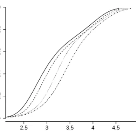
Figure 5: Cumulative distribution functions: 1970 (solid line), 1980 (dashed line), 1990 (dotted line) and 2000 (dashed-dotted line). X-axis: PPP US $ GDP/per capita, base year : 2000, scale 103. 0 0.2 0.4 0.6 0.8 1 2.5 3 3.5 4 4.5
Figure 6: Cumulative distribution functions: 1970 (solid line), 1980 (dashed line), 1990 (dotted line) and 2000 (dashed-dotted line). X-axis: log PPP US $ GDP/per capita, base year : 2000, log to the base 10.
Year Foster0 $1 Foster0 $2 World Popula-tion (in millions) Absolute Number of Poor below 1$ per day (in millions) Absolute Number of Poor below 2$ per day (in millions) Foster1 $1 Foster1 $2 1970 0.22 0.45 3,678 809 1,655 0.08 0.21 1975 0.2 0.44 4,061 812 1,787 0.07 0.2 1980 0.14 0.37 4,433 621 1,640 0.05 0.16 1985 0.08 0.28 4,825 386 1,351 0.03 0.1 1990 0.07 0.21 5,256 368 1,104 0.03 0.08 1995 0.07 0.17 5,668 397 963 0.03 0.07 2000 0.06 0.14 6,062 364 849 0.02 0.06 2003 0.05 0.14 6,290 314 881 0.02 0.06
Table 3: Poverty measures 1970-2003 Gini Pietra’s measure Atkinson, parameter 0.5 Theil’s en-tropy mea-sure Coefficient of variation Generalized entropy, parameter 0.5 1970 0.7 0.56 0.4 0.93 1.8 0.9 1975 0.7 0.56 0.41 0.94 1.82 0.92 1980 0.69 0.55 0.4 0.92 1.8 0.89 1985 0.68 0.54 0.38 0.9 1.85 0.85 1990 0.67 0.53 0.37 0.89 1.88 0.83 1995 0.66 0.51 0.36 0.85 1.82 0.79 2000 0.65 0.5 0.34 0.82 1.81 0.76 2003 0.64 0.49 0.34 0.79 1.76 0.75
Growth Rate in Mean Growth Rate at Median Mean Per-centile Growth Rate Rate of Pro-Poor Growth at P0= 469.9 Rate of Pro-Poor Growth at P0= 935.45 1970-2003 1.9 3.3 2.67 2.55 2.97 1970-1974 2.07 0.63 1.62 2.19 1.64 1975-1979 2.53 3.15 2.79 2.52 3 1980-1984 1.01 2.48 2.84 5.17 5.11 1985-1989 2.11 3.32 2.16 -0.72 1.11 1990-1994 1.44 3.06 2.12 1.04 1.53 1995-1999 2.37 3.45 2.8 2.7 2.51 2000-2003 1.29 2.19 1.7 0.82 0.94
Table 5: Growth facts 1970-2003
0
1
2
3
4
Growth Rates in Precent
0 20 40 60 80 100
Percentiles
Growth incidence curve Growth rate in mean Mean of growth rates ppgr
1970−2003
Growth Incidence Curve
.5 1 1.5 2 2.5 3
Growth Rates in Precent
0 20 40 60 80 100
Percentiles
1970−1974
Growth Incidence Curve
0
1
2
3
4
Growth Rates in Precent
0 20 40 60 80 100
Percentiles
1975−1979
Growth Incidence Curve
0
2
4
6
Growth Rates in Precent
0 20 40 60 80 100
Percentiles
1980−1984
Growth Incidence Curve
−2
0
2
4
Growth Rates in Precent
0 20 40 60 80 100
Percentiles
1985−1989
Growth Incidence Curve
.5 1 1.5 2 2.5 3
Growth Rates in Precent
0 20 40 60 80 100
Percentiles
1990−1994
Growth Incidence Curve
1.5
2
2.5
3
3.5
Growth Rates in Precent
0 20 40 60 80 100
Percentiles
1995−1999
Growth Incidence Curve
.5
1
1.5
2
2.5
Growth Rates in Precent
0 20 40 60 80 100
Percentiles
2000−2003
Growth Incidence Curve