Introduction to Stochastic Actor-Based Models
for Network Dynamics
∗
Tom A.B. Snijders
†Gerhard G. van de Bunt
‡Christian E.G. Steglich
§Abstract
Stochastic actor-based models are models for network dynamics that can represent a wide variety of influences on network change, and allow to es-timate parameters expressing such influences, and test corresponding hy-potheses. The nodes in the network represent social actors, and the collec-tion of ties represents a social relacollec-tion. The assumpcollec-tions posit that the net-work evolves as a stochastic process ‘driven by the actors’, i.e., the model lends itself especially for representing theories about how actors change their outgoing ties. The probabilities of tie changes are in part endogenously determined, i.e., as a function of the current network structure itself, and in part exogenously, as a function of characteristics of the nodes (‘actor covari-ates’) and of characteristics of pairs of nodes (‘dyadic covaricovari-ates’). In an extended form, stochastic actor-based models can be used to analyze longi-tudinal data on social networks jointly with changing attributes of the actors: dynamics of networks and behavior.
This paper gives an introduction to stochastic actor-based models for dynamics of directed networks, using only a minimum of mathematics. The focus is on understanding the basic principles of the model, understanding the results, and on sensible rules for model selection.
Keywords:statistical modeling, longitudinal, Markov chain, agent-based model, peer selection, peer influence.
∗Draft article for special issue of Social Networks onDynamics of Social Networks. We are grateful to Andrea Knecht who collected the data used in the example, under the guidance of Chris Baerveldt. We also are grateful to Matthew Checkley and two reviewers for their very helpful remarks on earlier drafts.
†University of Oxford and University of Groningen ‡Free University, Amsterdam
1. Introduction
Social networks are dynamic by nature. Ties are established, they may flourish and perhaps evolve into close relationships, and they can also dissolve quietly, or suddenly turn sour and go with a bang. These relational changes may be con-sidered the result of the structural positions of the actors within the network – e.g., when friends of friends become friends–, characteristics of the actors (‘actor covariates’), characteristics of pairs of actors (‘dyadic covariates’), and residual random influences representing unexplained influences. Social network research has in recent years paid increasing attention to network dynamics, as is shown, e.g., by the three special issues devoted to this topic in Journal of Mathematical Sociologyedited by Patrick Doreian and Frans Stokman (1996, 2001, and 2003; also see Doreian and Stokman, 1997). The three issues shed light on the under-lying theoretical micro mechanisms that induce the evolution of social network structures on the macro level. Network dynamics is important for domains rang-ing from friendship networks (e.g., Pearson and Michell, 2000; Burk, Steglich, and Snijders, 2007) to, for example, organizational networks (see the review ar-ticles Borgatti and Foster, 2003; Brass, Galaskiewicz, Greve, and Tsai, 2004). In this article we give a tutorial introduction to what we call here stochas-tic actor-based models for network dynamics, which are a type of models that have the purpose to represent network dynamics on the basis of observed longi-tudinal data, and evaluate these according to the paradigm of statistical inference. This means that the models should be able to represent network dynamics as be-ing driven by many different tendencies, such as the micro mechanisms alluded to above, which could have been theoretically derived and/or empirically estab-lished in earlier research, and which may well operate simultaneously. Some ex-amples of such tendencies are reciprocity, transitivity, homophily, and assortative matching, as will be elaborated below. In this way, the models should be able to give a good representation of the stochastic dependence between the creation, and possibly termination, of different network ties. These stochastic actor-based models allow to test hypotheses about these tendencies, and to estimate param-eters expressing their strengths, while controlling for other tendencies (which in statistical terminology might be called ‘confounders’).
The literature on network dynamics has generated a large variety of mathe-matical models. To describe the place in the literature of stochastic actor-based models (Snijders 1996, 2001), these models may be contrasted with other dynamic network models.
Most network dynamics models in the literature pay attention to a very spe-cific set of micro mechanisms –allowing detailed analyses of the properties of these models–, but lack an explicit estimation theory. Examples are models
pro-posed by Bala and Goyal (2000), Hummon (2000), Skyrms and Pemantle (2000), and Marsili, Vega-Redondo, and Slanina (2004), all being actor-based simulation models that focus on the expression of a single social theory as reflected, e.g., by a simple utility function; those proposed by Jin, Girvan, and Newman (2001) which represent a larger but still quite restricted number of tendencies; and models such as those proposed by Price (1976), Barab´asi and Albert (1999), and Jackson and Rogers (2007), which are actor-based, represent one or a restricted set of tenden-cies, and assume that nodes are added sequentially while existing ties cannot be deleted, which is a severe limitation to the type of longitudinal data that may be faithfully represented. Since such models do not allow to control for other influ-ences on the network dynamics, and how to estimate and test parameters is not clear for them, they cannot be used for purposes of theory testing in a statistical model.
The earlier literature does contain some statistical dynamic network mod-els, mainly those developed by Wasserman (1979) and Wasserman and Iacobucci (1988), but these do not allow complicated dependencies between ties such as are generated by transitive closure. Further there are papers that present an empiri-cal analysis of network dynamics which are based on intricate and illuminating descriptions such as Holme, Edling, and Liljeros (2004) and Kossinets and Watts (2006), but which are not based on an explicit stochastic model for the network dynamics and therefore do not allow to control one tendency for other (‘confound-ing’) tendencies.
Distinguishing characteristics of stochastic actor-based models are flexibility, allowing to incorporate a wide variety of actor-driven micro mechanisms influ-encing tie formation; and the availability of procedures for estimating and testing parameters that also allow to assess the effect of a given mechanism while control-ling for the possible simultaneous operation of other mechanisms or tendencies. We assume here that the empirical data consist of two, but preferably more, repeated observations of a social network on a given set of actors; one could call thisnetwork panel data. Ties are supposed to be the dyadic constituents of rela-tions such as friendship, trust, or cooperation, directed from one actor to another. In our examples social actors are individuals, but they could also be firms, coun-tries, etc. The ties are supposed to be, in principle, under control of the send-ing actor (although this will be subject to constraints), which will exclude most types of relations where negotiations are required for a tie to come into existence. Actor covariates may be constant like sex or ethnicity, or subject to change like opinions, attitudes, or lifestyle behaviors. Actor covariates often are among the determinants of actor similarity (e.g., same sex or ethnicity) or spatial proximity between actors (e.g., same neighborhood) which influence the existence of ties.
Dyadic covariates likewise may be constant, such as determined by kinship or formal status in an organization, or changing over time, like friendship between parents of children or task dependencies within organizations.
This paper is organized as follows. In the next section, we present the assump-tions of the actor-based model. The heart of the model is the so-called objective function, which determines probabilistically the tie changes made by the actors. One could say that it captures all theoretically relevant information the actors need to ‘evaluate’ their collection of ties. Some of the potential components of this function are structure-based (endogenous effects), such as the tendency to form reciprocal relations, others are attribute-based (exogenous effects), such as the preference for similar others. In Section 3 we discuss several statistical is-sues, such as data requirements and how to test and select the appropriate model. Following this we present an example about friendship dynamics, focusing on the interpretation of the parameters. Section 4 proposes some more elaborate models. In Section 5, models for the coevolution of networks and behavior are introduced and illustrated by an example. Section 6 discusses the difference between equilib-rium and out-of-equilibequilib-rium situations, and how these longitudinal models relate to cross-sectional statistical modeling of social networks. Finally, in Section 7, a brief discussion is given, theSienasoftware is mentioned which implements these methods, and some further developments are presented.
2. Model assumptions
A dynamic network consists of ties between actors that change over time. A foundational assumption of the models discussed in this paper is that the network ties are not briefevents, but can be regarded asstates with a tendency to endure over time. Many relations commonly studied in network analysis naturally satisfy this requirement of gradual change, such as friendship, trust, and cooperation. Other networks more strongly resemble ‘event data’, e.g., the set of all telephone calls among a group of actors at any given time point, or the set of all e-mails being sent at any given time point. While it is meaningful to interpret these networks as indicators of communication, it is not plausible to treat their ties as enduring states, although it often is possible to aggregate event intensity over a certain period and then view these aggregates as indicators of states.
Given that the network ties under study denote states, it is further assumed, as an approximation, that the changing network can be interpreted as the outcome of a Markov process, i.e., that for any point in time, the current state of the net-work determines probabilistically its further evolution, and there are no additional effects of the earlier past. All relevant information is therefore assumed to be in-cluded in the current state. This assumption often can be made more plausible by
choosing meaningful independent variables that incorporate relevant information from the past.
This paper gives a non-technical introduction into actor-based models for net-work dynamics. More precise explanations can be found in Snijders (2001, 2005) and Snijders, Steglich, and Schweinberger (2007). However, a modicum of math-ematical notation cannot be avoided. The tie variables are binary variables, de-noted by xij. A tie from actor i to actor j, denoted i → j, is either present or
absent (xij then having values 1 and 0, respectively). Although this is in line with
traditional network analysis, an extension to valued networks would often be the-oretically sound, and could make the Markov assumption more plausible. This is one of the topics of current research. The tie variables constitute the network, rep-resented by itsn×nadjacency matrixx= xij
(self-ties are excluded), wheren
is the total number of actors. The changes in these tie variables are the dependent variables in the analysis.
2.1. Basic assumptions
The model is about directed relations, where each tiei → j has a senderi, who will be referred to as ego, and a receiver j, referred to as alter. The following assumptions are made.
1. The underlying time parametert is continuous, i.e., the process unfolds in time steps of varying length, which could be arbitrarily small. The param-eter estimation procedure, however, assumes that the network is observed only at two or more discrete points in time. The observations can also be referred to as ‘network panel waves’, analogous to panel surveys in non-network studies.
This assumption was proposed already by Holland and Leinhardt (1977), and elaborated by Wasserman (1979 and other publications) and Leenders (1995 and other publications) – but their models represented only reci-procity, and no other structural dependencies between network ties. The continuous-time assumption allows to represent dependencies between net-work ties as the result of processes where one tie is formed as a reaction to the existence of other ties. If, for example, three actors who at the first ob-servation are mutually disconnected form at the second obob-servation a closed triangle, where each is connected to both of the others, then a discrete-time model that has the observations as its time steps would have to account for the fact that this closed triangle structure is formed ‘out of nothing’, in one time step. In our model such a closed triangle can be formed tie by tie, as a consequence of reciprocation and transitive closure. Thus, the appearance
of closed triangles may be explained based on reciprocity and transitive pro-cesses, without requiring a special process specifically for closed triangles.
Since many small changes can add up to large differences between con-secutively observed networks, this does not preclude that what is observed shows large changes from one observation to the next.
2. The changing network is the outcome of a Markov process. This was ex-plained above. Thus, the total network structure is the social context that influences the probabilities of its own change.
The assumption of a Markov process has been made in practically all mod-els for social network dynamics, starting by Katz and Proctor’s (1959) dis-crete Markov chain model. This is an assumption that will usually not be realistic, but it is difficult to come up with manageable models that do not make it. We could say that this assumption is a lens through which we look at the data – it should help but it also may distort. If there are only two panel waves, then the data have virtually no information to test this assumption. For more panel waves, there is in principle the possibility to test this as-sumption and propose models making less restrictive asas-sumption about the time dependence, but this will require quite complicated models.
3. The actors control their outgoing ties. This means not that actors can change their outgoing ties at will, but that changes in ties are made by the actors who send the tie, on the basis of their and others’ attributes, their position in the network, and their perceptions about the rest of the network. This assumption is the reason for using the term ‘actor-based model’. This ap-proach to modeling is in line with the methodological apap-proach of structural individualism (Udehn, 2002; Hedstr¨om, 2005), where actors are assumed to be purposeful and to behave subject to structural constraints. The assump-tion of purposeful actors is not required, however, but a quesassump-tion of model interpretation (see below).
It is assumed formally that actors have full information about the network and the other actors. In practice, as can be concluded from the specifica-tions given below, the actors only need more limited information, because the probabilities of network changes by an actor depend on the personal net-work (including actors’ attributes) that would result from making any given change, or possibly the personal network including those to whom the actor has ties through one intermediary (i.e., at geodesic distance two).
4. At a given moment one probabilistically selected actor – ‘ego’ – may get the opportunity to change one outgoing tie. No more than one tie can change at
any moment – a principle first proposed by Holland and Leinhardt (1977). This principle decomposes the change process into its smallest possible components, thereby allowing for relatively simple modelling. This implies that tie changes are not coordinated, and depend on each other only sequen-tially, via the changing configuration of the whole network. For example, two actors cannot decide jointly to form a reciprocal tie; if two actors are not tied at one observation and mutually tied at the next, then one of the must have taken the initiative and extended a one-sided tie, after which, at some later moment, the other actor reciprocated and formed a reciprocal tie. This assumption excludes relational dynamics where some kind of coordination or negotiation is essential for the creation of a tie, or networks created by groups participating in some activity, such as joint authorship networks. For directed networks, this usually is a reasonable simplifying assumption. In most cases, panel data of directed networks have many tie differences between successive observations and do not provide information about the order in which ties were created or terminated, so that this is an assumption about which the available data contain hardly any empirical evidence. Summarizing the status of these four basic assumptions: the first (continuous-time model) makes sense intuitively; the second (Markov process) is an as-if ap-proximation and it would be interesting in future to construct models going be-yond this assumption; the third (actor-based) is often a helpful theoretical heuris-tic; and the fourth (ties change one by one) is an assumption which limits the applicability to a wide class of panel data of directed networks for which this assumption seems relatively harmless.
The actor-based network change process is decomposed into two sub-processes, both of which are stochastic.
5. The change opportunity process, modeling the frequency of tie changes by actors. The change rates may depend on the network positions of the actors (e.g., centrality) and on actor covariates (e.g., age and sex).
6. The change determination process, modeling the precise tie changes made when an actor has the opportunity to make a change. The probabilities of tie changes may depend on the network positions, as well as covariates, of ego and the other actors (‘alters’) in the network. This is explained below. The actor-based model can be regarded as an agent-based simulation model (Macy and Willer 2002). It does not deviate in principle from other agent-based models, only in ways deriving from the fact that the model is to be used for statis-tical inference, which leads to requirements of flexibility (enough parameters that can be estimated from the data to achieve a good fit between model and data) and
parsimony (not more fine detail in the model than what can be estimated from the data). The word ‘actor’ rather than ‘agent’ is used, in line with other sociolog-ical literature (e.g., Hedstr¨om 2005), to underline that actors are not regarded as subservient to others’ interests in any way.
The actor-based model, when elaborated for a practical application, contains parameters that have to be estimated from observed data by a statistical procedure. Since the proposed stochastic models are too complex for the straightforward ap-plication of classical estimation methods such as maximum likelihood, Snijders (1996, 2001) proposed a procedure using the method of moments implemented by computer simulation of the network change process. This procedure uses the basic principle that the first observed network is itself not modeled but used only as the starting point of the simulations. In statistical terminology: the estimation procedure conditions on the first observation. This implies that it is the change between two observed periods time points that is being modeled, and the analysis does not have the aim to make inferences about the determinants of the network structure at the first time point.
2.2. Change determination model
The first step in the model is the choice of the focal actor (ego) who gets the op-portunity to make a change. This choice can be made with equal probabilities or with probabilities depending on attributes or network position, as elaborated in Section 4.1. This selected focal actor then may change one outgoing tie (i.e., either initiate or withdraw a tie), or do nothing (i.e., keep the present status quo). This means that the set of admissible actions containsnelements: n−1changes and one non-change. The probabilities for a choice depend on the so-called ob-jective function. This is a function of the network, as perceived by the focal actor. Informally, the objective function expresses how likely it is for the actor to change her/his network in a particular way. On average, each actor ‘tries to’ move into a direction of higher values of her/his objective function, subject to the constraints of the current network structure and the changes made by the other actors in the network; and subject to random influences. The objective function will depend in practice on the personal network of the actor, as defined by the network be-tween the focal actor plus those to whom there is a direct tie (or, depending on the specification, the focal actor plus those to whom there is a direct or indirect – i.e., distance-two – tie), including the covariates for all actors in this personal network. Thus, the probabilities of changes are assumed to depend on the per-sonal networks that would result from the changes that possibly could be made, and their composition in terms of covariates, via the objective function values of those networks.
core of model and it must represent the research questions and relevant theoretical and field-related knowledge. The objective function is explained in more detail in the next section.
The name ‘objective function’ was chosen because one possible interpretation is that it represents the short-term objectives (net result of preferences and struc-tural as well as cognitive constraints) of the actor. Which action to choose out of the set of admissible actions, given that ego has the opportunity to act (i.e., change a network tie), follows the logic of discrete choice models (McFadden, 1973; Maddala, 1983) which have been developed for modeling situations where the dependent variable is a choice made from a finite set of actions.
2.3. Specification of the objective function
The objective function determines the probabilities of change in the network, given that an actor has the opportunity to make a change. One could say it rep-resents the ‘rules for network behavior’ of the actor. This function is defined on the set of possible states of the network, as perceived from the point of view of the focal actor, where ‘state of the network’ refers not only to the ties but also to the covariates. When the actor has the possibility of moving to one out of a set of network states, the probability of any given move is higher accordingly as the objective function for that state is higher.
Like in generalized linear statistical models, the objective function is assumed to be a linear combination of a set of components calledeffects,
fi(β, x) =
X
k
βkski(x). (1)
In this section and elsewhere, the symbol i and the term ‘ego’ are ways of re-ferring to the focal actor. Here fi(β, x)is the value of the objective function for
actoridepending on the statexof the network; the functionsski(x)are the effects,
functions of the network that are chosen based on theory and subject-matter know-ledge, and correspond to the ‘tendencies’ mentioned in the introductory section; and the weights βk are the statistical parameters. The effects represent aspects
of the network as ‘viewed’ from the point of view of actor i. As examples, one can think of the number of reciprocated ties of actor i, representing tendencies toward reciprocity, or the number of ties fromitoward actors of the same gender, representing tendencies toward gender homophily. Many more examples are pre-sented below. The effects ski(x) depend on the networkx but may also depend
on actor attributes (actor covariates), on variables depending on pairs of actors (dyadic covariates), etc. Ifβk equals 0, the corresponding effect plays no role in
moving into directions where the corresponding effect is higher, and the converse ifβkis negative.
For the model selection, an essential part is the theory-guided choice of ef-fects included in the objective function in order to test the formulated hypotheses. A good approach may be to progressively build up the model according to the method of decreasing abstraction (Lindenberg, 1992). An additional considera-tion here is, however, that the complexity of network processes, and the limitaconsidera-tions of our current knowledge concerning network dynamics, imply that model con-struction may require data-driven elements to select the most appropriate precise specification of the endogenous network effects. For example, in the investiga-tion of friendship networks one might be interested in effects of lifestyle variables and background characteristics on friendship, while recognizing the necessity to control for tendencies toward reciprocation and transitive closure. As discussed below in the section on triadic effects, multiple mathematical specifications are available (as ‘effects’ski(x)to be included in equation (1)) expressing the concept
of transitive closure. Usually there are no prior theoretical or empirical reasons for choosing among these specifications. It may then be best to use theoretical considerations for deciding to include lifestyle-related and background variables as well as tendencies toward reciprocation and transitive closure in the model, and to choose the best specification for transitive closure, by one or several specific effects, in a data-driven way.
In the following we give a number of effects that may be considered for in-clusion in the objective function. They are described here only conceptually, with some brief pointers to empirical results or theories that might support them; the formulae are given in the appendix. Effects depending only on the network are called structural or endogenous effects, while effects depending only on exter-nally given attributes are called covariateor exogenous effects. The complexity of networks is such that an exhaustive list cannot meaningfully be given. To sim-plify formulations, the presentation shall assume that the relation under study is friendship, so the existence of a tiei→j will be described asicallingja friend. Higher values of the objective function, leading to higher tendencies to form ties, will sometimes be interpreted in shorthand as preferences.
Basic effects
The most basic effect is defined by the outdegree of actor i, and this will be in-cluded in all models. It represents the basic tendency to have ties at all, and in a decision-theoretic approach its parameter could be regarded as the balance of benefits and costs of an arbitrary tie. Most networks are sparse (i.e., they have a density well below 0.5) which can be represented by saying that for a tie to an arbitrary other actor – arbitrary meaning here that the other actor has no charac-teristics or tie pattern making him/her especially attractive to i –, the costs will
usually outweigh the benefits. Indeed, in most cases a negative parameter is ob-tained for the outdegree effect.
Another quite basic effect is the tendency towardreciprocity, represented by the number of reciprocated ties of actor i. This is a basic feature of most social networks (cf. Wasserman and Faust, 1994, Chapter 13) and usually we obtain quite high values for its parameter, e.g., between 1 and 2.
Transitivity and other triadic effects
Next to reciprocity, an essential feature in most social networks is the tendency toward transitivity, or transitive closure (sometimes called clustering): friends of friends become friends, or in graph-theoretic terminology: two-paths tend to be, or to become, closed (e.g., Davis 1970, Holland and Leinhardt 1971). In Figure 1.a, the two-pathi→j →his closed by the tiei→h.
Figure 1. a. Transitive triplet(i, j, h) b. Three-cycle
i h j i h j
Thetransitive tripletseffect measures transitivity for an actoriby counting the number of pairsj, hsuch that there is the transitive triplet structure of Figure 1.a. However, this is just one way of measuring transitivity. Another one is the transi-tive tieseffect, which measures transitivity for actoriby counting the number of other actors h for which there is at least one intermediary j forming a transitive triplet of this kind. The transitive triplets effect postulates that more intermediaries will add proportionately to the tendency to transitive closure, whereas the transi-tive ties effect expects that given that one intermediary exists, extra intermediaries will not further contribute to the tendency to forming the tiei→h.
An effect closely related to transitivity isbalance(cf. Newcomb, 1962), which in our implementation is the same as structural equivalence with respect to out-ties(cf. Burt, 1982), which is the tendency to have and create ties to other actors who make the same choices as ego. The extent to which two actors make the same choices can be expressed simply as the number of outgoing choices and non-choices that they have in common.
Transitivity can be represented by still more effects: e.g., negatively, by the number of others to whomi is indirectly tied but not directly (geodesic distance equal to 2). The choice between these representations of transitivity may depend
both on the degree to which the representation is theoretically convincing, and on what gives the best fit.
A different triadic effect is the number of three-cycles that actoriis involved in (Figure 1.b). Davis (1970) found that in many social network data sets, there is a tendency to have relatively few three-cycles, which can be represented here by a negative parameter βk for the three-cycle effect. The transitive triplets and the
three-cycle effects both represent closed structures, but whereas the former is in line with a hierarchical ordering, the latter goes against such an ordering. If the network has a strong hierarchical tendency, one expects a positive parameter for transitivity and a negative for three-cycles. Note that a positive three-cycle effect can also be interpreted, depending on the context of application, as a tendency toward generalized exchange (Bearman, 1997).
Degree-related effects
In- and outdegrees are primary characteristics of nodal position and can be impor-tant driving factors in the network dynamics.
One pair of effects isdegree-related popularity based on indegree or outde-gree. If these effects are positive, nodes with higher indegree, or higher outdegree, are more attractive for others to send a tie to. This can be measured by the sum of indegrees of the targets of i’s outgoing ties, and the sum of their outdegrees, respectively. A positive indegree-related popularity effect implies that high inde-grees reinforce themselves, which will lead to a relatively high dispersion of the indegrees (a Matthew effect in popularity as measured by indegrees, cf. Merton, 1968 and Price, 1976). A positive outdegree-related popularity effect will increase the association between indegrees and outdegrees, or keep this association rela-tively high if it is high already.
Another pair of effects is degree-related activity for indegree or outdegree: when these effects are positive, nodes with higher indegree, or higher outdegree respectively, will have an extra propensity to form ties to others. These effects can be measured by the indegree of i times i’s outdegree; and, respectively, the outdegree of i times i’s outdegree, that is, the square of the outdegree.1 The
outdegree-related activity effect again is a self-reinforcing effect: when it has a positive parameter, the dispersion of outdegrees will tend to increase over time, or to be sustained if it already is high. The indegree-related activity effect has the same consequence as the outdegree-related popularity effect: positive parameters lead to a relatively high association between indegrees and outdegrees. There-fore these two effects will be difficult, or impossible, to distinguish empirically,
1Experience has shown that for the degree-related effects, often the ‘driving force’ is measured better by the square roots of the degrees than by raw degrees. In some cases this may be supported by arguments about diminishing returns of increasingly high degrees. See the formulae in the appendix.
and the choice between them will have to be made on theoretical grounds. These four degree-related effects can be regarded as the analogues in the case of directed relations of what was calledcumulative advantageby Price (1976) and preferen-tial attachment by Barab´asi and Albert (1999) in their models for dynamics of non-directed networks: a self-reinforcing process of degree differentiation.
These degree-related effects can represent hierarchy between nodes in the net-work, but in a different way than the triadic effects of transitivity and 3-cycles. The degree-related effects represent global hierarchy while the triadic effects re-present local hierarchy. In a perfect hierarchy, ties go from the bottom to the top, so that the bottom nodes have high outdegrees and low indegrees and the top nodes have low outdegrees and high indegrees. This will be reflected by positive indegree popularity and negative outdegree popularity, and by positive outdegree activity and negative indegree activity. Therefore, to differentiate between local and global hierarchical processes, it can be interesting to estimate models with triadic and degree-related effects, and assess which of these have the better fit by testing the triadic parameters while controlling for the degree-related parameters, and vice versa.
Other degree-related effects areassortativity-related: actors might have pref-erences for other actors based on their own and the other’s degrees (Morris and Kretzschmar 1995; Newman 2002). In settings where degrees reflect status of the actors, such preferences may be argued theoretically based on status-specific preferences, constraints, or matching processes. This gives four possibilities, de-pending on in- and outdegree of the focal actor and the potential friend.
Together, this list offers eight degree-related effects. The outdegree-related popularity and indegree-related activity effects are nearly collinear, and it was al-ready mentioned that theory, not empirical fit, will have to decide which one is a more meaningful representation. Some of the other effects also may be con-founded, but this depends on the data set. The four effects described as degree-related popularity and activity are more basic than the assortativity effects (cf. the relation between main effects and interactions in linear regression). Because of this, when testing any assortativity effects, one usually should control for three of the degree-related popularity and activity effects.
Covariates: exogenous effects
For an actor variable V, there are three basic effects: the ego effect, measuring whether actors with higher V values tend to nominate more friends and hence have a higher outdegree (which also can be called covariate-related activity ef-fect or sender efef-fect); the alter effect, measuring whether actors with higher V
values will tend to be nominated by more others and hence have higher indegrees (covariate-related popularity effect, receiver effect); and thesimilarity effect, mea-suring whether ties tend to occur more often between actors with similar values on
V (homophily effect). Tendencies to homophily constitute a fundamental charac-teristic of many social relations, see McPherson, Smith-Lovin, and Cook (2001). When the ego and alter effects are included, instead of the similarity effect one could use theego-alter interaction effect, which expresses that actors with higher
V values have a greater preference for other actors who likewise have higher V
values.
For categorical actor variables, the same V effect measures the tendency to have ties between actors with exactly the same value ofV.
For a dyadic covariate, i.e., a variable defined for pairs of actors, there is one basic effect, expressing the extent to which a tie between two actors is more likely when the dyadic covariate is larger.
Interactions
Like in other statistical models, interactions can be important to express theo-retically interesting hypotheses. The diversity of functions that could be used as effects makes it difficult to give general expressions for interactions. The ego-alter interaction effect for an actor covariate, mentioned above, is one example.
Another example is given by de Federico (2004) as an interaction of a covari-ate with reciprocity. In her analysis of a friendship network between exchange stu-dents, she found a negative interaction between reciprocity and having the same nationality. Having the same nationality has a positive main effect, reflecting that it is easier to become friends with those coming from the same country. The nega-tive interaction effect was unexpected, but can be explained by regarding recipro-cation as a response to an initially unreciprocated tie, the latter being a unilateral invitation to friendship. Since contacts between those with the same national-ity are easier than between individuals from different nationalities, extending a unilateral invitation to friendship is more remarkable (and perhaps more costly) between individuals of different nationalities than between those of the same na-tionality. Therefore it will be noticed and appreciated, and hence reciprocated, with a higher probability. Thus, the rarity of cross-national friendships leads to a stronger tendency to reciprocation in cross-national than same-nationality friend-ships.
As a further class of examples, note that in the actor-based framework it may be natural to hypothesize that the strength of certain effects depends on attributes of the focal actor. For example, girls might have a greater tendency toward transi-tive closure than boys. This can be modeled by the interaction of the ego effect of the attribute and the transitive triplets, or transitive ties effect.
Other interactions (and still other effects) are discussed in Snijders et al. (2008). As the selection presented here already illustrates, the portfolio of possible effects in this modeling approach is very extensive, naturally reflecting the multitude of possibilities by which networks can evolve over time. Therefore, the selection
of meaningful effects for the analysis of any given data set is vital. This will be discussed now.
3. Issues arising in statistical modeling
When employing these models, important practical issues are the question how to specify the model – boiling down mainly to the choice of the terms in the objective function – and how to interpret the results. This is treated in the current section.
3.1. Data requirements
To apply this model, the assumptions should be plausible in an approximate sense, and the data should contain enough information. Although rules of thumb always must be taken with many grains of salt, we first give some numbers to indicate the sizes of data sets which might be well treated by this model. These rules of thumb are based on practical experience.
The amount of information depends on the number of actors, the number of observation moments (‘panel waves’), and the total number of changes between consecutive observations. The number of observation moments should be at least 2, and is usually much less than 10. There are no objections in principle against analyzing a larger number of time points, but then one should check the assump-tion that the parameters in the objective funcassump-tion are constant over time, or that the trends in these parameters are well represented by their interactions with time variables (see point 10 below).
If one has more than two observation points, then in practice one may wish to start by analyzing the transitions between each consecutive pair of observations (provided these provide enough information for good estimation – see below). For each parameter one then can present the trend in estimated parameter values, and depending on this one can make an analysis of a larger stretch of observations if the parameters appear approximately constant, or do the same while including for some of the parameters an interaction with a time variable.
The number of actors will usually be larger than 20 – but if the data contain many waves, a smaller number of actors could be acceptable. The number of ac-tors will usually not be more than a few hundred, because the implicit assumption that each actor is a potential network partner for any other actor might be implau-sible for networks with so many actors that not all actors are aware of each others’ existence.
The total number of changes between consecutive observations should be large enough, because these changes provide the information for estimating the param-eters. A total of 40 changes (cumulated over all successive panel waves) is on
the low side. More changes will give more information and, thereby, allow more complicated models to be fitted. Between any pair of consecutive waves, the num-ber of changes should not be too high, because this would call into question the assumption that the waves are consecutive observations of a gradually changing network; or, if they were, the consecutive observations would be too far apart.
This implies that, when designing the study, the researcher has to have a rea-sonable estimate of how much change to expect. For instance, if one is inter-ested in the development of the friendship network of a group of initially mutual strangers (e.g., university freshmen), it may be good to plan the observation mo-ments to be separated by only a few weeks, and to enlarge the period between observations after a couple of months. On the other hand, if one studies inter-firm network dynamics, given the time delays involved for firms in the planning and executing of their ties to other firms, it may be enough to collect data once every year, or even less frequently.
To express quantitatively whether the data collection points are not too far apart, one may use the Jaccard (1900) index (also see Batagelj and Bren, 1995), applied to tie variables. This measures the amount of change between two waves by
N11
N11+N01+N10
, (2)
whereN11 is the number of ties present at both waves, N01is the number of ties newly created, and N10 is the number of ties terminated. Experience has shown that Jaccard values between consecutive waves should preferably be higher than .3, and – unless the first wave has a much lower density than the second – values less than .2 would lead to doubts about the assumption that the change process is gradual, compared to the observation frequency. If the network is in a period of growth and the second network has many more ties than the first, one may look instead at the proportion, among the ties present at a given observation, of ties that have remained in existence at the next observation (N11/(N10+N11)in the preceding notation). Proportions higher than .6 are preferable, between .3 and .6 would be low but may still be acceptable. If the data collection was such that values of ties (ranging from weak to strong) were collected, then these numbers may be used as rough rules of thumb and give some guidance for the decision where to dichotomize the tie values – although, of course, substantive concerns related to the interpretation of the results have primacy for such decisions.
The methods require in principle that network data are complete. However, it is allowed that some of the actors enter the network after the start, or leave before the end of the panel waves (Huisman and Snijders, 2003), and a limited amount of missing data can be accommodated (Huisman and Steglich, 2008). Another option to represent that some actors are not yet, or no more, present in the
net-work, is to specify that certain ties cannot exist (‘structural zeros’) or that some ties are prescribed (‘structural ones’), see Snijders et al. (2008). The use of struc-tural zeros allows, e.g., to combine several small networks into one structure (with structural zeros forbidding ties between different networks), allowing to analyze multiple independent networks that on themselves would not yield enough in-formation for estimating parameters, under the extra assumption that all network follow dynamics with the same parameter values in the objective function.
3.2. Testing and model selection
It turns out (supported by computer simulations) that the distributions of the esti-mates of the parameters βk in the objective function (1), representing the
impor-tance of the various terms mentioned in Section 2.3, are approximately normally distributed. Therefore these parameters can be tested by referring thet-ratio, de-fined as parameter estimate divided by standard error, to a standard normal distri-bution.
For actor-based models for network dynamics, information-theoretic model selection criteria have not yet generally been developed, although Koskinen (2004) presents some first steps for such an approach. Currently the best possibility is to use ad hoc stepwise procedures, combining forward steps (where effects are added to the model) with backward steps (where effects are deleted). The steps can be based on significance test for the various effects that may be included in the model. Guidelines for such procedures are the following. We prefer not to give a recipe, but rather a list of considerations that a researcher might have in mind when constructing a strategy for model selection.
1. Like in all statistical models, exclusion of one effect may mask the existence of another effect, so that pure forward selection may lead to overlooking some effects, and it is advisable to start with a model including all effects that are expected to be strong.
2. Fitting complicated models may be time-consuming and lead to instability of the algorithm, and a resulting failure to obtain good estimates. Therefore, forward selection is technically easier than backward selection, which is unfortunately at variance with the preceding remark.
3. The estimation algorithm (Snijders, 2001) is iterative, and the initial value can determine whether or not the algorithm converges. For relatively simple models, a simple standard initial value usually works fine. For complicated models, however, the algorithm may converge more easily if started from an initial value obtained as the estimate for a somewhat simpler model. Es-timates obtained from a more complicated model by simply omitting the
deleted effects sometimes do not provide good starting values. Therefore, forward selection steps often work better from the algorithmic point of view than backward steps. This implies that, to improve the performance of the algorithm, it is advisable to retain copies of the parameter values obtained from good model fits, for use as possible initial values later on.
4. Network statistics can be highly correlated just because of their definition. This also implies that parameter estimates can be rather strongly correlated, and high parameter correlations do not necessarily imply that some of the effects should be dropped. For example, the parameter for the outdegree effect often is highly correlated with various other structural parameters. This correlation tells us that there is a trade-off between these parameters and will lead to increased standard errors of the parameter for the outdegree effect, but it is not a reason for dropping this effect from the model.
5. Parameters can be tested by a so-called score-type test without estimating them, as explained in Schweinberger (2008). Since estimating many pa-rameters can make the algorithm instable, and in forward selection steps it may be necessary to have tests available for several effects to choose the most important one to include, the score-type tests can be very helpful in model selection. In this procedure, a model (null hypothesis) including sig-nificant and/or theoretically relevant parameters is tested against a model (alternative hypothesis) extended by one or several parameters one is also interested in. Under the null hypothesis, those parameters are zero. The procedure yields a test statistic with a chi-squared null distribution, along with standard normal test statistics for each separate parameter. The param-eters for which a significant test result was found, then may be added to the model for a next estimation round.
6. It is important to let the model selection be guided by theory, subject-matter knowledge, and common sense. Often, however, theory and prior know-ledge are stronger with respect to effects of covariates – e.g., homophily effects – than with respect to structure. Since a satisfactory fit is important for obtaining generalizable results, the structural side of model selection will of necessity often be more of an inductive nature than the selection of covariate effects. The newness of this method implies that we still need to accumulate more experience as to what is a ‘satisfactory’ fit, and how complicated models should be in practice.
7. Among the structural effects, the outdegree and reciprocity effect should be included by default. In almost all longitudinal social network data sets, there also is an important tendency toward transitivity (Davis 1970). This should
be modeled by one, or several, of the transitivity-related effects described above.
8. Often, there are some covariate effects which are predicted by theory; these may be control effects or effects occurring in hypotheses. It is good prac-tice to include control effects from the start. Non-significant control effects might be dropped provisionally and then tested again as a check in the pre-sumed final model; but one might also retain control effects independent of their statistical significance. We do not think there are unequivocal rules whether or not to include from the start the effects representing the main hypotheses in a given study.
9. The degree-based effects (popularity, activity, assortativity) can be impor-tant structural alternatives for actor covariate effects, and can be imporimpor-tant network-level alternatives for the triad-level effects. It is advisable, at some moment during the model selection process, to check these effects; note that the square-root specification usually works best.
10. If the data have three or more waves and the model does not include time-changing variables, then the assumption is made that the time dynamics is homogeneous, which will lead to smooth trajectories of the main statistics from wave to wave. It is good as a first general check to consider how aver-age degree develops over the waves, and if this development does not follow a rather smooth curve (allowing for random disturbances), to include time-varying variables that can represent this development. Another possibility is to analyze consecutive pairs of waves first, which will show the extent of inhomogeneity in the process (cf. the example in Snijders, 2005).
11. The model assumes that the ‘rules for network change’ are the same for all actors, except for differences implied by covariates or network position. This leaves only moderate room for outlying actors, such as are indicated by relatively very large outdegrees or indegrees. Very high or very low outdegrees or indegrees should be ‘explainable’ from the model specifica-tion; if they are only explainable from earlier observations (‘path depen-dence’), they will have a tendency to regress toward the mean. The model specification may be able to explain outliers by covariates identifying ex-ceptional actors, but also by degree-related endogenous effects such as the self-reinforcing Matthew effect mentioned above. It is good as a first gen-eral check to inspect the indegrees and outdegrees for outliers. If there are strong outliers then it is advisable to seek for actor covariates which can help to explain the outlying values, or to investigate the possibility that degree-related effects, explainable or at least interpretable from a theoretical point
of view, may be able to represent these outlying degrees. If these cannot be found, then one solution is to use dummy variables for the actors con-cerned, to represent their outlying behavior. Such an ad hoc model adapta-tion, which may improve the fit dramatically, is better than the alternative of working with a model with a large unmodeled heterogeneity. In case there is a theoretical argument to expect certain outliers, these can be pointed out by including a dummy variable, but of a different kind. In contrast to the former type of outliers, the latter one is expected, so should be captured in advance by a covariate. If one is not capable to make a difference between the two types, one has to rely on the ad hoc model adaptation.
3.3. Example: friendship dynamics
By way of example, we analyze the evolution of a friendship network in a Dutch school class. The data were collected between September 2003 and June 2004 as part of a study reported in Knecht (2008). The 26 students were followed over their first year at secondary school during which friendship networks as well as other data were assessed at four time points at intervals of three months. There were 17 girls and 9 boys in the class, aged 11-13 at the beginning of the school year. Network data were assessed by asking students to indicate up to twelve classmates which they considered good friends. The average number of nomi-nated classmates ranged between 3.6 and 5.7 over the four waves, showing a mod-erate increase over time. Jaccard coefficients for similarity of ties between waves are between .4 and .5, which is somewhat low (reflecting fairly high turnover) but not too low.
Some data were missing due to absence of pupils at the moment of data col-lection. This was treated by ad-hoc model-based imputation using the procedure explained in Huisman and Steglich (2008). One pupil left the classroom. Such changes in network composition can also be treated by the methods of Huisman and Snijders (2003), but this simple case was treated here by usingstructural ze-ros: starting with the first observation moment where this pupil was not a member of the classroom any more, all incoming and outgoing tie variables of this pupil were fixed to zero and not allowed to change in the simulations.
Considering point 1 above, effects known to play a role in friendship dynam-ics, such as basic structural effects and effects of basic covariates, are included in the baseline model. From earlier research, it is known that friendship formation tends to be reciprocal, shows tendencies towards network closure, and in this age group is strongly segregated according to the sexes. The model includes, for each of these tendencies, effects corresponding to these expectations. Structural effects included are reciprocity; transitive triplets and transitive ties, measuring transitive closure that is compatible with an informal local hierarchy in the friendship
net-work; and the three-cycles effect measuring anti-hierarchical closure. Homophily based on the sexes is included as the same sex effect. All variables are centered. For example, the dummy variable for sex (boys = 1, girls = 0) has mean 0.346 (9 boys and 17 girls), which leads to the centered valuesvi = –0.346 for girls andvi
= 0.654 for boys.
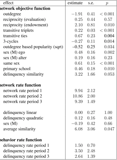
As exogenous control variables, we include sender and receiver effects of sex, and a dyadic covariate indicating friendship in primary school reflecting relation-ship history. In addition, several degree-related endogenous effects are included as control effects: in- and outdegree-related popularity, and outdegree-related ac-tivity, explained above. Estimates for this model are given in Table 1 as Model 0. All calculations were done using Siena version 3.2 (Snijders et al., 2008).
The parameters reported for the rate function in periods 1-3 are defined in the simulation model as the expected frequencies, between successive waves, with which actors get the opportunity to change a network tie. For these parameters no
p-values are given in the tables, as testing that they are zero is meaningless (if these would be zero there would be no change at all). These estimated rate parameters will be higher than the observed numbers of changes per actor, however, because in the model an actor may get the opportunity to change a tie but choose not to make any change, and because actors may add a tie during the simulations, and withdraw the same tie before the next observation moment.
Table 1 about here
This analysis confirms, for this data set, several of the known properties of friendship networks: there is a high degree of reciprocity, as seen in the signif-icant reciprocity parameter; there is segregation according to the sexes, as seen in the significant same sexparameter; there is an almost equally strong effect of having been friends at primary school already, and there is evidence for transitive closure, as seen in the significant effects of transitive tripletsand transitive ties. A direct comparison of the size of parameter estimates is possible, given that they occur in the same linear combination in the objective function, but it should be kept in mind that these are unstandardized coefficients. Other significant effects are the negative 3-cycles parameter, which indicates that the tendencies toward closure are not completely egalitarian (as one might have thought based on the reciprocity parameter), but do show some evidence for local hierarchization in the network. This also is suggested by the marginally significant negative effect of the outdegree-related popularity which indicates that active pupils, i.e., those who nominate particularly many friends, are less likely to be chosen as friends – this could be a status effect negatively associated with nomination activity. Also significant is the sender effect of sex (sex (M) ego), which in our coding of the variable means that the boys tend to be more active in the classroom friendship network than the girls.
Rate parameters, finally, suggest that the amount of friendship change seems to peak in the second period (perhaps due to a higher friendship turnover after the Christmas break) and slow down towards the end of the school year. These differences are small, however. The same descriptive conclusion can be drawn also by inspecting the observed amounts of change, without needing to refer to a statistical model.
In a subsequent model (Model 1 in Table 1), more parsimony is obtained by eliminating the non-significant effects in a backward selection procedure. The sex alter effect was retained in spite of its non-significance, because the three sex-related effects belong together as a representation of sex-sex-related friendship pref-erences. One by one, the least significant of the insignificant effects were dropped from the model. While doing so, score-type tests were made for the earlier omit-ted parameters (now constrained to zero) to check whether the parameter does not become significant upon dropping other effects from the model. This is possi-ble in models with correlated effects like ours, but it did not occur for our data set. Estimates of Model 1 give the same qualitative results as those of Model 0. The parameters dropped due to insignificance were the outdegree-related activity effect (suggesting that the value for ego of an individual friendship does not de-pend on how many other friends the friend currently has) and the indegree-related popularity effect (suggesting that receiving many friendship nominations is not a self-reinforcing process).
3.4. Parameter interpretation
For the general understanding of the numerical values of the parameters, it may be kept in mind that the parameters βk in the objective function are unstandardized
coefficients of the statistics of which the mathematical formulae are given in the appendix.
The parameters in the objective function can be interpreted in two ways. In the first place, by interpreting this function as the “attractiveness” of the network for a given actor. For getting a feeling of what are small and large values, it may be noted (see the interpretation in terms of myopic optimization in Snijders, 2001) that the objective functions are used to compare how attractive various different tie changes are, and for this purpose random disturbances are added to the values of the objective function with standard deviations equal2to 1.28.
The objective function is a weighted sum of effectssik(x); their mathematical
definitions are given in the appendix. In most cases the contribution of a single tie variablexij is just a simple component of this formula.
For example, consider the actor variable sex, denoted as V, and originally
2More exactly, the value isp
with values 1 for girls and 2 for boys. All variables are centered. The global mean of this variable is 1.346 (9 boys and 17 girls), which leads to the centered valuesvi =−0.346for girls andvi = 0.654for boys. For this variable the model
includes the ‘ego’ effect, the ‘alter’ effect, and the ‘same’ effect. Let us denote the parameters by βe,βa, and βs. Then, using the formulae in the appendix, the joint contribution of theseV-related effects to the objective function is
βe X j xijvi + βa X j xijvj + βs X j xijI{vi =vj}
whereI{vi = vj}= 1ifvi =vj, and 0 otherwise. This means that the
contribu-tion of the single tiexij to the objective function, considering only the sex-related
effects, is given by
βevi + βavj + βsI{vi =vj} = 0.35vi + 0.10vj + 0.49I{vi =vj}
Substituting the values -0.346 for females and 0.654 for males yields the following table.
alter
ego F M
F 0.33 –0.06
M 0.19 0.78
This table shows that girls as well as boys prefer friendships with same-sex alters, but for boys the difference is more pronounced than for girls.
A second interpretation is that when actor i has the opportunity to make a change in her outgoing ties (where no change also is an option), andxaandxbare
two possible results of this change, thenfi(xb, β)−fi(xa, β)is the log odds ratio
for choosing between these two alternatives – so that the ratio of the probability ofxbandxaas next states is
exp fi(xb, β)−fi(xa, β) = exp fi(xb, β) exp fi(xa, β) .
Note that, when the current state isx, the possibilities forxaandxbarexitself (no
change), orx with one extra outgoing tie fromi, orx with one less outgoing tie fromi. Explanations about log odds ratios can be found in texts about logistic re-gression and loglinear models, e.g., Agresti (2002). A further elaborated example of this is given below in Section 4.2.
4. More complicated models
This section treats two generalizations of the model sketched above.
4.1. Differential rates of change: the rate function
Depending on actor attributes or on positional characteristics such as indegree or outdegree, actors might change their ties at differential frequencies. This can be the case, e.g., in networks between organizations with clear differences in degrees, where the outdegrees reflect the importance to the organizations of the network under study, and the resources they devote to positioning themselves in it. The average frequency at which actors get the opportunity to change their outgoing ties then is called therate function, depending on attributes and network position of the actors.
Model 2 in Table 1 gives an example of such an analysis. It extends Model 1 by adding an effect of sex on the rate function. The estimated negative effect indicates that in the data set under study, boys change their network ties less frequently than girls, but the difference is not significant (p= 0.13).
To interpret the parameter values, one should know that a so-called exponen-tial link function is used (Snijders, 2001; Snijders et al., 2008), which means that the variables have an effect on the rate function after an exponential transforma-tion, with a multiplicative effect. For example, the parameter estimate of –0.42 for the effect of sex on the rate function implies that the estimated rate function is the base rate multiplied byexp(−0.42vi). Recall that the values of the variable ‘sex’
are, centered,vi =−0.346for females andvi = 0.654for males. Thus, for period
1, for girls the expected number of opportunities for change is9.69×exp(−0.42× (−0.346)) = 11.2, and for boys it is9.69×exp(−0.42×(0.654)) = 7.4. The difference seems rather large but is not significant in view of the small sample size.
4.2. Differences between creating and terminating ties: the endowment function
In the treatment given above, terminating a tie is just the opposite of creating one. This is not always a good representation of reality. It is conceivable, for example, that the loss when terminating a reciprocal tie is greater than the gain in creating one; or that transitive closure works especially for the creation of new ties, but hardly guards against termination of existing ties. This can be modeled by having two components of the objective function: theevaluation function, which considers only the network that will be the case as a result of the change to be made; and the endowment function, which is a component that operates only for the termination of ties and not for their creation. Everything discussed above about
the objective function concerned the evaluation function – in other words, in those discussions and the example, the endowment function was nil. The endowment function gives contributions to the objective function that do not play a role when creating ties, but that are lost when dissolving ties.
Model 3 in Table 1 gives the results of an analysis that includes, in addi-tion to the effects of Model 1, also an endowment effect related to reciprocity. It was estimated as significant and positive, while the corresponding evaluation function effect of reciprocity dropped in size and significance. To interpret this result, jointly consider the reciprocity evaluation effect with parameter 0.71 and the reciprocity endowment effect with parameter 1.42. The contribution of a tie being reciprocated then is 0.71 for the creation of the tie and 0.71 + 1.42 = 2.13 against the termination of the tie. Thus, reciprocity here is more important against terminating friendships – that is, for maintaining friendships – than for creating friendships.
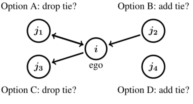
To elaborate this example, consider how the friendship choices of a girl to-wards other girls depend on reciprocity. Suppose that actor ican change one of her ties, while there are two girls j1 and j2, both of them choosingias a friend, and two others j3 and j4 not choosing i. In addition, suppose that currently i choosesj1 andj3as friends, but not the other two. Assume finally (artificially, for the sake of explanation) that these four girls do not choose each other and further also are isolated fromi’s network so that other structural effects besides recipro-city do not matter. Since the actor variable ‘sex’ has centered valuevi =−0.346
for girls, the parameter estimates for Model 3 give as the total contribution of the three sex-related effects for girl-girl ties 0.41vi + 0.16vj + 0.56I{vi = vj} = (0.41 + 0.16)×(−0.346) + 0.56 = 0.36. With the outdegree effect of –1.59, this yields−1.59 + 0.36 = −1.23as the basic contribution of a tie to the evaluation function.
Option A: drop tie? Option B: add tie?
Option C: drop tie? Option D: add tie? ego
i
j1 j2
j3 j4
Figure 2. Four options for actori.
When girlican change a tie variable, using this value of –1.23 for the combined effect of outdegree and the three sex-related effects for a girl-girl tie, five of the options foriare the following:
(A): drop reciprocated friendship tie toj1 : –(–1.23) – 2.13 = – 0.90; (B): reciprocate friendship tie fromj2 : –1.23 + 0.71 = –0.52; (C): drop non-reciprocated friendship tie toj3 : –(–1.23) = 1.23; (D): initiate friendship tie toj4 : –1.23;
(E): do nothing: 0.0.
Since these are contributions to logarithms of probabilities, the proportionality factors between the probabilities of these events must be calculated as the expo-nential transformations of these values, which are, respectively, e−0.90 = 0.41, 0.59, 3.42, 0.29, and 1.
These are the relative probabilities of changes toward any given other girl. One should note, however, that there may be different numbers of the four cases (A-D) for a given girl, and the probability of severinganyreciprocated tie, or of creatinganynon-reciprocated tie, depends also on these numbers for the ‘ego’ girl under consideration. Since the friendship network is sparse, with average degrees between 3.6 and 5.7, the cases of type (D) will be most numerous. Consider, for instance, a girl with 3 mutual girlfriends (A), who has 2 non-reciprocated friend-ships to girls (C), 1 other girl who mentions her as a friend without reciprocation (B), and 10 girls without a friendship either way (D). Suppose that in addition she has no friendships with any of the 9 boys, and denote the option of estab-lishing a friendship to a boy by (F). Retain the unrealistic simplifying assumption that all her network members are mutually unrelated, also after adding one hypo-thetical new friend, so that transitivity does not influence probabilities of change. The baseline value of a tie from a girl to a boy is −1.59 + 0.41×(−0.346) + 0.16× 0.654 = −1.63, with exponential transform 0.20. Taking into account the fact that the number of opportunities for options (A) to (F) are 3, 1, 2, 10, 1, and 9, the six proportionality factors have to be divided by the denominator
(3×0.41) + (1×0.59) + (2×3.42) + (10×0.29) + (1×1) + (9×0.20) = 14.36. Thus, for this girl, the probabilities are:
(A): of dropping any of the three reciprocated friendship ties:(3×0.41)/14.36 = 0.09;
(B): of reciprocating the incoming friendship tie: (1×0.59)/14.36 = 0.04;
(C): of dropping one of the non-reciprocated friendship ties: (2×3.42)/14.36 = 0.48;
(D): of initiating some new friendship tie to a girl: (10×0.29)/14.36 = 0.20;
(E): of doing nothing: 0.07;
(F): and of extending a new friendship tie to a boy: (9×0.20)/14.36 = 0.13. Thus, in line with theories about reciprocation such as balance theory, the prob-ability is slightly larger than 0.5 that the proportion of reciprocity in friendships will be increased. There are many random influences, however, that would de-crease reciprocity – but most of these are proposals of new ties which could be
seen by the other party as an invitation toward future reciprocation.
5. Dynamics of networks and behavior
Social networks are so important also because they are relevant for behavior and other actor-level outcomes: related actors may influence one another (e.g., Fried-kin, 1998), and ties will be selected in part based on the similarity between ego and potential relational partners (homophily, see McPherson, Smith-Lovin, and Cook, 2001). This means that not only is the network changing as a function of itself and of the actor variables, but likewise the actor variables are changing as a function of themselves and of the network. We use the termbehavioras shorthand for en-dogenously changing actor variables, although these could also refer to attitudes, performance, etc.; there could be one or more of such variables. It is assumed here that the behavior variables are ordinal discrete variables, with values 1, 2, etc., up to some maximum value, for instance, several levels of delinquency, several levels of smoking, etc. The dependence of the network dynamics on the total network-behavior configuration will be also called the social selectionprocess, while the dependence of the behavior dynamics on the total network-behavior configura-tion will be called thesocial influence process. Both social influence and social selection can lead to similarity between tied actors, which is often observed. A fundamental question then is whether this similarity is caused mainly by influence or mainly by selection, as discussed by Ennett and Bauman (1994) for smoking behavior and Haynie (2001) for delinquent behavior.
This combination of selection and influence can be modeled by an extension of the actor-based model to a structure where the dependent variables consist not only of the tie variables but also of the actors’ behavior variables, as specified in Snijders, Steglich and Schweinberger (2007) and Steglich, Snijders and Pearson (2009). Of course there usually will be, in addition, also exogenous actor and/or dyadic variables in the role of independent variables.
The assumptions for the actor-based model for the dynamics of networks and behavior are extensions of the assumptions for network dynamics. The extended formulations are as follows, given without the background explanations which were given above and which apply also for this case.
1. As above, the underlying time parameter is continuous.
2. The changing system consisting of network and behavior is the outcome of a Markov process. Thus, the probabilities of change of the network as well as those of the behavioral variables depend, at each moment, on the current combination of network structure and behavior variables for all actors.