The Trend in Retirement
Karen A. Kopecky1
The University of Western Ontario
July 2005
Version: September 2009
Abstract
A model with leisure production and endogenous retirement is used to explain the declining labor force participation rates of elderly males. The model is calibrated to cross-sectional data on the labor force participation rates of elderly US males by age, their median drop in market consumption and leisure good expenditure share in the year 2000. Running the calibrated model for the period 1850 to 2000, a prediction of the evolution of the cross-section is obtained. The model is able to predict more than 87 percent of the increase in retirement of men over 65. The increase in retirement is driven by rising real wages and a falling price of leisure goods over time.
JEL Classification Nos: E13, J26, O11, O33
Keywords: retirement, leisure, home production, consumption-drop, technological progress
Subject Area: Macroeconomics
1 I owe many thanks to Jeremy Greenwood. I would also like to thank the faculty and graduate students at the
University of Rochester, especially Mark Aguiar, Mark Bils, Fatih Guvenen, Guillaume Vandenbroucke and those who participated in the macro workshop and Jeremy’s first and second year macro classes; three anonymous referees; the editor; conference participants of the 2005 SITE “Nexus between Household Economics and the Macro Economy” workshop, the 2006 Labour Supply and Productivity Life Cycle Workshop at the Bank of Canada, the 2006 Midwest Macro Meetings, the 2006 SED meetings; and seminar participants at Concordia University, the Federal Reserve Banks of St. Louis, Dallas, Richmond, and Cleveland, the University of Guelph, York University, the University of Texas at San Antonio, Universidad Carlos III de Madrid, Cornell University, the University of Western Ontario, UCSB, Purdue Universiy, the University of Illinois at Urbana-Champaign, and Stanford University. All errors and inconsistencies are my own.
Address: Department of Economics, Social Science Centre, Room 4071 The University of Western Ontario,
London, ON, N6A 5C2, Canada. Email: [email protected].
1
Introduction
Senior citizens in the U.S. today spend their time gardening, travelling, and enjoying a wide range of entertainment goods. Less than 20 percent are in the workforce. Instead they allocate their time among various leisure and home activities. The U.S. was quite a different place in 1880, when more than 75 percent of men over the age of 65 were participating in the labor market. Labor force participation rates of men aged 65 and over have been continually declining since the latter half of the nineteenth century. Concurrently, life expectancies have risen resulting in an increase in the fraction of a man’s life spent in retirement.
Retired men spend the majority of their time engaged in leisure activities. Thus, the story of retirement is a story of leisure. Leisure activities, like most activities, require the use of both time and goods. Becker provides examples of such activities in his 1965 paper, one of which is “the seeing of a play, which depends on the input of actors, script, theatre and the playgoer’s time.”2 Another example is riding a bike which requires both time and a bike.
The quality-adjusted relative price of leisure goods has been declining since the nineteenth century. Over the same time period, real wage rates have been rising. The argument put forth here is that together declining leisure good prices and rising wages have made the leisure-intensive retirement lifestyle more affordable, driving a rise in retirement. The objective of the paper is to quantify the contributions of the rise in real wages and the fall in the prices of leisure goods to the decrease in the labor force participation rates of elderly U.S. males throughout the twentieth century.
To achieve this goal, a continuous-time model in which agents choose the moment of their retirement is developed. In the spirit of Becker (1965), agents in the model economy produce leisure by combining leisure time with leisure goods. When working, agents are assumed to work full-time and allocate remaining time to leisure production. Once retired agents allocate all their time to leisure production. Agents require a minimum level of market consumption for survival and derive utility from a non-separable function of leisure and consumption of market goods beyond subsistence level. The model is designed to be consistent with three important characteristics of the retirement period: (i.) upon retiring men significantly increase their time
spent on leisure activities; (ii.) for the majority of workers, retirement is a complete withdrawal from the labor force; and (iii.) for many individuals market consumption changes discretely at the moment of retirement.
The model permits leisure goods and leisure time to be either (Hicksian) substitutes or com-plements in leisure production. It is shown that when the two inputs are comcom-plements a fall in the price of leisure goods relative to leisure time will generate an increased demand for leisure time, lowering the optimal retirement age. In addition, it is shown that when leisure goods and leisure time are complements, the income effect of an increase in real wages dominates the substitution effect. Consequently, higher wages also lower the optimal retirement age. On the other hand, under substitutability between leisure time and leisure goods, a decrease in leisure good prices generates a rise in the optimal retirement age whereas an increase in wages has an ambiguous effect. The degree of complementarity between leisure goods and leisure time will not be assumed but determined by the calibration. Hence the calibration will determine both the overall and the relative importance of falling leisure good prices and rising wages for the increase in retirement observed in the data.
The model economy consists of overlapping generations of agents. In order to generate vari-ation in the age of retirement within a genervari-ation, agents differ by educvari-ation type and within education types they vary by initial market productivity level. Each agent has a hump-shaped market productivity profile which depends upon his birth year, education type and initial market productivity level and an age-specific survival function that depends upon his birth year. In addition, agents vary in their ability to produce leisure or leisure productivity which is constant over their lifetime and uncorrelated with their market productivity profile. Agents with higher education levels on average have higher levels of market productivity and profiles that peak later in life.
The effect of an increase in an agent’s overall level of market productivity is equivalent to the effect of an increase in wages. Therefore, everything else identical, agents with higher overall levels of market productivity will choose to retire earlier than those with lower ones whenever the income effect of an increase in wages dominates the substitution effect. The later peak in the higher types’ profiles however will increase the marginal cost of retiring at a given age relative to the cost for an agent with an earlier peaking profile. This is because the level of earnings that the agent
foregoes to retire is higher. Consequently while variation in education types and productivity levels within types will generate variation in retirement ages, the relationship between education type, initial market productivity, and retirement age will depend on the calibration.
Everything else identical, agents with higher leisure productivity will retire later than those with lower leisure productivity when leisure time and leisure goods are complements and vice versa when they are substitutes. When leisure time and leisure goods are complements agents with higher leisure productivity demand more leisure goods at each moment of their life. Thus it is optimal for them to delay retirement in order to increase their lifetime earnings and, consequently, their expenditure on leisure goods. When leisure time and leisure goods are substitutes it is the lower productivity agents that have a higher demand for leisure goods and therefore choose to retire relatively later.
The model is calibrated to the year 2000 using cross-sectional data from the Health and Retirement Study (HRS). The calibration is done by minimizing the distance between the model and data along eight key moments: the labor force participation rates of six age groups, the median drop in consumption at retirement, and leisure goods’ expenditure share. Then the model is used to compute the labor force participation rates of the six age groups over the 1850 to 2000 period by plugging in the rate of decrease of leisure good prices and the rate of increase of wages along with the changes in agents survival profiles, life expectancies, and education levels over this period.
The model is able to match the year 2000 distribution of elderly labor force participation rates by age group and generates a consumption drop at retirement and leisure good expenditure share in 2000 that are in line with the data. Under the baseline calibration, leisure time and leisure goods are complements and thus the fall in the relative price of leisure goods and the rise in wages over the 1850 to 2000 period have a positive impact on retirement. An increase in the fraction of agents with high school and college educations also positively impacts retirement. However, the effect of rising education is small. Finally, under the assumption that agents can fully insure against survival risk, rising life expectancies in the model have a negative impact on retirement.
According to the model, taking into account the observed changes in survival profiles, life expectancies and education levels since the eighteenth century, the rising wage rate and falling
prices of leisure goods explain more than 87 percent of the rise in retirement of males aged 65 and over. The model also reveals that these driving forces had a large impact on the retirement behavior of men aged 55 to 64. A series of counterfactual experiments show that the rise in real wages was the dominant force decreasing labor force participation rates. However, the decrease in the price of leisure goods since the eighteenth century has also played a significant role, alone generating approximately 13 percent of the increase in retirement of the elderly ages 65 to 69.
This paper is a first attempt at accounting for the long-run rise in retirement using a quan-titative macroeconomic approach. Similar arguments on the impact of leisure goods’ prices on labor-supply have been made to understand changes in labor-supply on the intensive margin by Owen (1971) and more recently by Vandenbroucke (2009) and Gonz´alez Chapela (2007). The argument that a fall in the price of leisure goods may be an important driver of the long-run rise in retirement was first made by Costa (1998). The most common alternative theory of rising retirement is that it was driven by the increase in social insurance programs and private pensions. However, findings from empirical studies on the ability of such programs to account for the rise are mixed.
The paper proceeds as follows: Section 2 presents some facts on retirement and leisure. Section 3 presents the model. The quantitative experiment is presented in Section 4, which includes of explanation of the calibration procedure and presents the model’s prediction for the trend in retirement since 1850. The section concludes with the presentation of a series of counterfactual experiments and a discussion of the contribution of the various driving forces to the retirement trend. Section 5 discusses related literature and Section 6 concludes.
2
Retirement
Retirement is defined as a planned, complete, and usually permanent withdrawal from the labor force by older workers. In this section, data illustrating the trends in retirement in the U.S. and other countries is presented. The section then provides a discussion of some important charac-teristics of the retirement period that are used as guidelines for making modeling assumptions.
1840 1860 1880 1900 1920 1940 1960 1980 2000 0 20 40 60 80 100 Germany US 55-64 US 65+ France L a b o r F o r c e P a r t i c i p a t i o n R a t e ( % ) Year Britain
Figure 1: Labor force participation rates of men aged 65 and over for the period 1850 to 1990 in the United States, France, Great Britain, and Germany and men aged 55 to 64 in the United States.
2.1 Historical Trends
A trend of rising retirement since the nineteenth century is not unique to the United States. Figure 1 shows the labor force participation rates of men aged 65 and over for the period 1850 to 1990 in the U.S., France, Great Britain, and Germany, and the participation rates of men aged 55 to 64 in the U.S. Notice that the decline in the labor force participation rates occurred in all four countries. This decline cannot be accounted for by the change in the composition of the elderly population due to the increase in life expectancy. Participation rates fell for all ages above 65. In addition, participation rates have fallen among men aged 55 to 64. In 1880, 96 percent of men aged 60 to 64 were in the labor force, by 1990 only 39 percent were. For men in their late fifties, participation rates have been declining since 1900 but started to decline at a faster rate around 1960.3
Labor force participation rates have also been declining in developing countries. For example, the labor force participation rate of men aged 65 and over fell from 67 percent to 52 percent in Mexico between 1970 and 1999. In Peru it fell from 62 percent to 41 percent and in Turkey from
3 See Costa (1998), Chapter 2 for a in-depth discussion of trends in labor force participation. The source for
1850 1880 1910 1940 1970 2000 0 15 30 45 60 75 90 1850 1880 1910 1940 1970 2000 5 10 15 20 25 30 Ages 70-74 Ages 55-59 Ages 65-69 Ages 60-64 Ages 50-54 R e t i r e m e n t R a t e ( % ) Year Ages 75-79 E x p e c t e d P e r c e n t a g e o f L i f e S p e n t i n R e t i r e m e n t Year
Figure 2: Retirement rates for men aged 50 and over by age group and the expected percentage of life spent in retirement at the age of 20 for the period 1850 to 2000 in the United States.
68 percent to 34 percent over the same period. Unfortunately data from these countries is only available for recent years.4
To obtain a direct measure of the increase in retirement a statistic called the retirement rate is calculated using data from IPUMS for men aged 50 and over for the period 1850 to 2000. The retirement rate is the ratio of the number of men who are retired to the number of men either in the labor force or retired. In order to be classed as retired a man must be completely out of the labor force. Hence men who are working part-time or part-year are counted as working and not retired. The retirement rates are presented in the left-hand graph of Figure 2 for men by five-year-age groups.5 Notice that the retirement rates of the youngest age group, those aged 50
to 54, don’t increase over time while the rates of all the other age groups do increase. For the oldest age group, those aged 75 to 79, the retirement rate rises from about 20 percent in 1850 to nearly 90 percent in 2000.
The combination of rising life expectancies and declining labor force participation rates of the elderly has led to an increase in the expected duration of retirement. In fact, a twenty-year-old
4 Source: U.S. Census Bureau, Series P95/01-1,An Aging World: 2001 (2001).
5 The data for the retirement rates is from: Ruggles, Steven, et al. 2004. Integrated Public Use
Micro-data Series: Version 3.0. (IPUMS) Minneapolis, MN: Minnesota Population Center. It can be found
at http://www.ipums.org. The retirement rates for each age group were computed by observing that:
male in 1850 would have expected to spend approximately 6 percent of his adult life retired, while a male who was twenty in 1990 can expect to spend 30 percent of adult life retired. The right-hand graph in Figure 2 shows how the expected percentage of adult life spent in retirement has risen over this period.6
2.2 Characteristics of the Retirement Period
In order to study the impact of changing prices on the retirement behavior of men a model of retirement must be consistent with the defining characteristics of the retirement period. Three important characteristics are discussed below along with an explanation of how the baseline model is designed to be in accordance with them.
2.2.1 Increase in Leisure
The retirement period is a period in which one must reallocate his time from market to non-market activities. Thus to gain insight into the retirement decision it is important to investigate how retired people spend their time. Table 1 gives a breakdown of men’s time-use by age.7 Notice
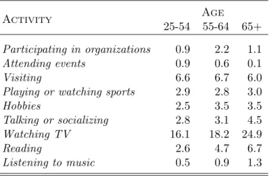
that older men allocate more of their time to leisure and home activities. In particular, men age 55 to 64 spend approximately 19 percent more time on recreation than men aged 25 to 54, while men age 65 and over spend nearly 43 percent more time. Thus retirement is a period when men’s time spent on leisure activities significantly increases. Consistent with this fact, retired men spend more time using leisure goods, such as televisions, radios, stereos, books, magazines, and newspapers. For example, according to Godbey and Robinson (1997), in 1985, men aged 55 to 64 spent 13 percent more time watching television than men aged 25 to 54, while men over the age of 64 spent 81 percent more time. Men over the age of 64 also spent nearly double the amount of time men aged 25 to 54 spent reading and listening to music. Table 2 gives a breakdown of time spent in various leisure activities by age groups for men in 1985.8 In addition to spending more time with leisure goods, there is evidence that upon retirement, individuals increase the share of
6 Adult life excludes the first twenty years. The data for the expected portion of life in retirement in Figure 2 is
taken from Lee (2001), Table 1, p. 645. It is based on the same IPUMS data as used to compute the retirement rates. The expected length of retirement is computed assuming 20 year-olds have perfect information about future mortality rates.
7 Source for Table 1 is Godbey and Robinson (1997), p. 207, Table 19.
Table 1: Hours per week spent in various activities for men by age group in 1985. Activity Age 25-54 55-64 65+ Sleeping 54.9 57.5 58.7 Working or commuting 40.1 23.7 8.0 Recreation 35.8 42.7 51.1
Grooming and child care 10.9 10.2 12.3
Eating and preparing meals 9.5 12 12.6
House and Yard Work 9.2 13.5 16.7
Shopping 4.7 5.4 5.6
Other 2.1 2 2.4
Table 2: Hours per week spent in various leisure activities for men by age group in 1985.
Activity Age
25-54 55-64 65+
Participating in organizations 0.9 2.2 1.1
Attending events 0.9 0.6 0.1
Visiting 6.6 6.7 6.0
Playing or watching sports 2.9 2.8 3.0
Hobbies 2.5 3.5 3.5
Talking or socializing 2.8 3.1 4.5
Watching TV 16.1 18.2 24.9
Reading 2.6 4.7 6.7
Listening to music 0.5 0.9 1.3
their expenditure that they allocate to leisure goods. Weagley and Huh (2004) find, using data from the 1995 Consumer Expenditure Survey, that controlling for age, education, income, and demographics, leisure goods’ share of total expenditure increases at retirement.
How have leisure good prices changed over time? The left-hand side of Figure 3 presents the price index for a particular selection of leisure goods relative to the CPI over the period 1900 to 2000. The price of these leisure goods has fallen at an average annual rate of approximately 1 percent.9 The price index is based on the set of leisure goods whose expenditure shares are
9 Sources for the price index: For the period 1901 to 1934, data from Owen (1969), Table 4-B, p. 85 is used; for
the period 1935 to 1968, data is from the Historical Statistics Series E 165; and for 1969 - 2001, the data is taken from the Bureau of Labor Statistics’ Handbooks of U.S. Labor Statistics, 2nd. Ed. (1998), p. 263 and 6th Ed. (2003), p. 308.
1900 1920 1940 1960 1980 2000 0.5 0.6 0.7 0.8 0.9 1.0 Year P r i c e I n d e x 1900 1920 1940 1960 1980 2000 0 1 2 3 4 5 6 7 8 9 Books/Maps Magazines/New spapers Nondurable Toys Durable Toys/ Sports Equipm ent Multim edia Equipm ent Flowers and Plants
P e r c e n t o f T o t a l E x p e n d i t u r e Year Admission Tickets
Figure 3: Relative price index of leisure goods and breakdown of their share of total expenditure in the United States for the period 1900 to 2001.
provided in the graph on the right-hand side.10 In 1900 the average American allocated
approxi-mately 3 percent of his expenditure to leisure goods. By 2001 this fraction had increased to over 8 percent. Notice that this set of leisure good does not include transportation goods or services. Yet approximately 30 percent of the average total miles driven with a car each year are driven for social and recreational trips.11 When 30 percent of expenditure on transportation is included
in leisure good expenditure, leisure goods’ expenditure share rises from about 4 percent in 1900 to nearly 12 percent in 2001.
To capture the effect of men’s reallocation of time from market activities to leisure activities upon retirement, it is assumed that men engage in leisure production. The notion of leisure production is inspired by Becker’s 1965 paper and is similar to home production. There is an extensive literature demonstrating the importance of home production in explaining a variety of phenomena.12 The key difference between home and leisure production is the following. Time spent on housework and household durables are usually found to be substitutes in production of the home good. Thus a fall in the price of household durables decreases the demand for time
10 The source for the expenditure shares is Lebergott (1996).
11 Based on data from a selection of years between 1951 and 1995. Source: 1951-58: U.S. Department of Commerce,
Bureau of Public Roads. 1969-1995: Federal Highway Administration, National Personal Transportation Survey, Summary of Travel Trends.
12 For examples see Reid (1934), Benhabib, Rogerson and Wright (1991), Greenwood, Seshadri and Vandenbroucke
spent on housework. In contrast, time spent on leisure activities and leisure goods are argued here to be complements in the production of leisure. Under this assumption, a fall in the price of leisure goods leads to an increased demand for leisure time.
2.2.2 Labor Force Withdrawal
For the majority of workers retirement involves a complete withdrawal from the labor force or, in other words, switching from full-time work to being fully retired. A variety of theories have been proposed to explain why a majority of older workers withdraw once and completely from the labor market. They include the inability of older workers, in demanding jobs, to handle physical and/or mental stress, minimum hours constraints and schedule inflexibility, and employer incentives and pensions. Evidence from the HRS has pointed to minimum hours constraints and schedule inflexibility as the largest factors influencing retirement decisions. For example, Hurd and McGarry (1993) find, using the HRS, that the ability to change hours of work, pensions, and health insurance have an important effect on retirement decisions. While Gustman and Steinmeier (2004) conclude, based on the HRS, that relaxing minimum hours constraints would significantly increase the percentage of older people who continue working. Given these findings, it is assumed that agents in the model start off their lives as workers and are unable to adjust labor supply on the intensive margin. Consequently, agents in the model are either working full-time or retired.
2.2.3 Drop in Market Consumption
Numerous studies based on a variety of different datasets have found evidence of a significant drop in consumption at the moment of retirement. The causes of this drop are not well understood and thus is has come to be known as the retirement-consumption puzzle. In contrast to these studies, in a recent work, Hurd and Rohwedder (2008) find an average consumption drop for individuals of 4.7 percent of pre-retirement expenditure and a median drop of 5.9 percent. Their estimates are based on data from the HRS and three waves of a supplemental survey called CAMS. Their analysis is unique in that it is the first study of the consumption drop at retirement for U.S. households that is based on observations of total expenditure before and after retirement by the
same individuals. The findings are in contrast to those of earlier works that used synthetic panels and/or partial measures of consumption and estimated the average drop in market expenditure to be in the range of 10 to 30 percent of pre-retirement expenditure.13 Exploring the distribution
of the expenditure drop across individuals, Hurd and Rohwedder (2008) find that estimates based on synthetic cohorts are likely to have been driven by a few individuals having large declines. They also find a great deal of variation in expenditure changes at retirement across the population with some individuals experiencing significant increases and others significant decreases.
One possible explanation for the discrete changes in expenditure at retirement observed in the data is that they are driven by complementarity or substitutability in utility between non-market time and various market goods. Supporting this view, Aguiar and Hurst (2005) find that while expenditure on food declines at retirement, calorie and vitamin consumption does not, suggesting that retirees substitute non-market time for expenditure on food. The findings of Weagley and Huh (2004) that leisure goods expenditures increase at retirement support the notion that leisure goods and non-market time are complements in utility.
Complementarity (or substitutability) in utility, also known as Edgeworth-Pareto complemen-tarity, is different from Hicksian complementarity. Two items are complements (substitutes) in utility if an increase in the amount of one item, increases (decreases) the marginal utility of the other. Whereas, two items are Hicksian complements (substitutes) if a decrease in the price of one increases (decrease) demand for the other. For two items to be Edgeworth-Pareto comple-ments or substitutes they must be nonseparable in utility such that their marginal utilities are functions of the level of the other item. When this is the case, it is optimal to discretely adjust the level of one item in response to a discrete jump in the level of the other in order to smooth utility. Whether two goods are complements or substitutes in utility depends upon the elasticity of substitution between the two items and the concavity of the utility function.
In the model economy total expenditure consists of expenditure on leisure goods and a general consumption good. Agents are assumed to produce leisure by combining leisure time with leisure
13 For example, Hurd and Rohwedder (2005) find, using data from the 2001 CAMS supplemental survey of 2000
HRS respondents that expenditure on market non-durables drops by 16.8 percent for singles and 11.6 percent for married couples at the moment of retirement of the household head, Bernheim, Skinner and Weinberg (2001) find an average drop in expenditure on food of 14 percent using data from the Panel Study of Income Dynamics and Aguiar and Hurst (2005) find an average drop in expenditures on food of 17 percent using data from the Continuing Survey of Food Intakes conducted by the U.S. Department of Agriculture.
goods and the production function is such that leisure time and leisure goods can be either Hicksian substitutes or complements with one another. In this framework the marginal utility of leisure time will depend on the quantity of leisure goods and vice versa. When agents retire their leisure time jumps up generating a discrete jump in their leisure good consumption. If utility is separable in market consumption and leisure, then the jump in leisure good consumption will drive the change in total consumption at the moment of retirement. However, as mentioned above, leisure good expenditure increases at retirement. In order to give the model the chance to be consistent with this fact and match the drop in total expenditure observed in the data, market consumption and leisure are assumed to be non-separable in utility.
3
The Model
Time is continuous and indexed by t. The economy consists of overlapping generations. Agents are characterized by their types≡(τ , e, x0, z), whereτ denotes the date of the agent’s birth. An
agent born at moment τ will be age a= t−τ at time t. The parameter e denotes the agent’s level of education and x0 is the agent’s initial market productivity level. Together τ,e, and x0
determine the agent’s lifetime market productivity profilexs(·). The parameter z is the agent’s ability to produce leisure and is constant over the agent’s lifetime.
Within each generation there is a distribution of agents across education levels and for each education level there is a distribution of agents across initial market productivity levels. Let Fτ(e) denote the distribution of generation-τ agents across education levels and Ge(x0) denote the distribution of agents of education level e across initial productivity levels. Each agent’s leisure productivity, z, is drawn from the distribution H(z) which is independent of the agent’s age-cohort, education level, and initial market productivity. In addition, there is no correlation between an agent’s market ability profile and his leisure ability.
Agents live for a maximum length of timeT. At ages belowT an agent’s survival is determined by a generation-specific survival function qτ(a). In other words, qτ(a) is the probability that a member of the generation-τ cohort survives to at least age a.
The economy contains two types of goods: market (or general consumption) goods and goods which aid in leisure production, here called leisure goods. The price of market goods at each date
t is normalized to one. The price of leisure goods relative to market goods at datet is denoted by pg(t).
3.1 Agents’ Maximization Problem
Agents have one unit of time at each moment of their lives. Newly-born agents of type s start off their lives as workers, inelastically supplying a fraction ¯h of their time to the market and receiving earnings w(τ +a)¯hxs(a). The function w(τ +a) is the wage per an efficiency unit of labor at time τ +a and xs(a) is the agents’ market productivity at age a. Market productivity profiles are humped-shaped over the life-cycle.
Time that is not spent working on the market is dedicated to the production of leisure which requires both time and leisure goods. At each age a, each agent combines leisure with market goods to generate utility. In addition to choosing the stream of market goods, cs(a), and the stream of leisure goods, gs(a), that he purchases over his lifetime, a type-s agent chooses an age at which to permanently retire from market work, As. Once retired agents spend all their time on leisure production. Thus time spent on leisure production by a type-sagent is defined as
ls(a) = 1−¯h, a≤As, 1, a > As. (3.1)
Leisure time and leisure goods are combined to produce leisure using the constant elasticity of substitution production function
ns(a) ={ζgs(a)χ+ (1−ζ)[zls(a)]χ}
1
χ,
where 0≤ζ ≤1,χ≤1 andχ= 0 implies a Cobb-Douglas production function. The parameter ζ is the weight on leisure inputs relative to leisure time in the production function. Under this formulation the elasticity of substitution between leisure time and leisure goods is 1/(1−χ).
An agent born at date τ with education level e, initial market productivity x0 and leisure
productivity z chooses paths of market good and leisure good purchases over his lifetime,cs(a) andgs(a),respectively, and the age of his retirement,As, to maximize his expected lifetime utility
given by
Z As
0
e−θaqτ(a)U[cs(a), ns(a)]da+ Z T
As
e−θaqτ(a)U[cs(a), ns(a)]da, (3.2)
subject to his lifetime budget constraint and A ≤T. The parameter θ captures the subjective time-discounting rate and the cohort-dependent survival function,qτ(a) is log-sextic in age. The momentary utility function is of the constant relative risk aversion form so
U[cs(a), ns(a)] =
©
[cs(a)−c]ˆαns(a)1−α
ª1−σ
1−σ , (3.3)
where ˆc ≥0, 0 ≤ α ≤1, σ > 0 and σ = 1 implies log-utility. The parameter α determines the importance of market goods relative to leisure for utility and the parameter ˆc is a subsistence level of market good consumption. The objective function is expressed as the sum of the agent’s utility while working and his utility while retired. This is done to highlight the role that the age at which the agent retires, a choice variable, plays in his decision problem. It is also written in this way because, as is described below, time spent on leisure is not continuous at the moment of retirement. In general, the discontinuity in leisure time at retirement will result in a discontinuity in the momentary utility function at retirement.
As in Kalemli-Ozcan, Ryder and Weil (2000), the economy contains a life-insurance company which offers actuarially-fair annuities to the agents. Annuities allow agents to share mortality risk and, as was first shown by Yaari (1965), since the agents have no bequest motive or precautionary savings motive they will use annuities as their sole instrument of investment. The rate of return on an annuity for an agent with death hazard rate hτ(a) = −dlnqτ(a)/da is equal to r, the risk-free rate, plus hτ(a). Thus the agent’s lifetime budget constraint is
RAs 0 e−raqτ(a)cs(a)da+ RT Ase −raq τ(a)cs(a)da+ RAs 0 e−raqτ(a)pg(a+τ)gs(a)da+ RT Ase −raq τ(a)pg(a+τ)gs(a)da= RAs
0 e−raqτ(a)xs(a)¯hw(a+τ)da.
(3.4)
Hereafter thes-subscript is dropped for ease of notations.
The first-order condition for market consumption is
where λ is the multiplier on (3.4) in the Lagrangian. The first-order condition for purchase of the leisure good is
(1−α)ζe−θa[c(a)−c]ˆ(1−σ)αn(a)(1−σ)(1−α)−χg(a)χ−1 =
λe−rapg(a+τ), ∀a∈[0, T].
(3.6)
Notice that time spent on leisure enters the first-order conditions for market consumption and leisure goods. This occurs because market consumption and leisure time are non-separable in utility as are leisure goods and leisure time. Hence leisure time affects the marginal utility of market consumption and leisure goods. Agents want to smooth marginal utility over their lifetime. However, at the moment of retirement their marginal utility jumps discretely due to the discrete jump in their leisure time. In order to smooth marginal utility, the agents make discrete adjustments to their consumption and leisure goods at this moment. The first-order condition for the retirement age is
{[cA−ˆc]αn1A−α} 1−σ 1−σ − {[cA−cˆ]αn1A−α} 1−σ 1−σ ≤λe(θ−r)A £ x(A)¯hw(A+τ)−(cA−cA) −pg(A+τ)(gA−gA) i , (3.7)
wherecAis market consumption at the moment of retirement, given that the agent is still working, or
cA=c(A), (3.8)
cA is defined as
cA= lim
a→A+c(a), (3.9)
and nA, nA, gA, and gA, are defined similarly. To understand equation (3.7), consider the problem of an agent who is deciding whether or not he should retire at age A. If he retires, his instantaneous utility changes. His net gain in utility is on the left-hand side of equation (3.7). This is the marginal cost of postponing retirement. The right-hand side is the marginal benefit. It is the utility value of the savings of the agent at ageAif he is working net of his savings atAif he is retired. As long as the marginal benefit of working exceeds the marginal cost, the agent will not retire. Thus an agent could die having never retired. At an interior solution for the optimal retirement date, A, equation (3.7) will hold with equality.
Solving (3.5) for c(a) and differentiating with respect toagives ˙ c(a) c(a)−ˆc = 1 Φ · θ−r−Ψn(a)˙ n(a) ¸ , (3.10) where Φ = (1−σ)α−1, and Ψ = (1−σ)(1−α).
Totally differentiating (3.6) with respect to gand a, plugging in (3.10), and rearranging yields
˙ g(a) g(a) = µ ˙ pg(a+τ) pg(a+τ) − θ−r Φ ¶ . µ χ−1−ζ µ Ψ Φ +χ ¶ · g(a) n(a) ¸χ¶ . (3.11)
The stream of market goods and leisure goods that agents purchase over the lifetime must satisfy the differential equations given by equations (3.10) and (3.11).
Under what conditions will falling prices of leisure goods and rising wages generate an increase in retirement? First consider the effect of a fall in the price of leisure goods. The lower price will lead to an increase in retirement when χ <0. In this case leisure time and leisure goods will be complements and a decrease in the price of leisure goods will generate an increased demand for leisure time. Leisure time, however, can only be increased by retiring earlier. Thus agents will choose to exit the labor force at a younger age. In the opposite case, χ >0, leisure goods and leisure time are substitutes and a decrease in the price of leisure goods will delay retirement.
Now consider the impact on retirement of an increase in wages. The impact can be decomposed into two effects. The first effect is due to the fact that, when the wage rate increases, the price of leisure goods relative to leisure time falls. This has the same effect on retirement as a fall in the price of leisure goods: If χ <0 then it will lower the retirement age and ifχ >0 it will raise the retirement age. The second effect is due to the fact that the price of market consumption relative to leisure time falls. As long as ˆc >0 market goods and leisure time will be complements and the fall in this price will lower the retirement age. If ˆc = 0 then the retirement age is independent of the relative price. Hence, overall, an increase in wages will lead to an increase in retirement if χ ≤ 0. However, when χ > 0 the two effects work in opposite directions and, depending on
which effect dominates, retirement will either decrease or increase. These results are formalized in the following two propositions. Formal proofs are provided in the Appendix for the case where σ = 1. Although not proven here, the results hold for the general case ofσ >0. In the numerical exercise that follows whether χis positive or negative will be determined by the calibration.
Proposition 1 Let the path of leisure good prices over the agent’s lifetime be pg(a+ τ) = pg,τp˜g(a+τ). Then, at an interior solution, the retirement age A is
i. independent ofpg,τ if χ= 0,
ii. increasing inpg,τ if leisure goods and leisure time are complements (χ <0),
iii. decreasing in pg,τ if leisure goods and leisure time are substitutes (χ >0).
Proof. See the Appendix for the proof whenσ= 1.
Proposition 2 Let the path of wages over the the agent’s lifetime be w(a+τ) = wτw(a˜ +τ).
Then, at an interior solution withχ≤0, the retirement ageA is decreasing in wτ.
Proof. See the Appendix for the proof whenσ= 1.
Variation in market productivity profiles and leisure productivity will generate a variation in retirement rates within generations. An agent’s retirement age will depend upon both the level and the shape of his productivity profile. Notice that the effect on retirement age of a higher level of market productivity, holding the shape of the profile fixed, is equivalent to the effect of an upward shift in an agent’s lifetime wage profile. Thus, holding the shape fixed, agents with higher levels of market productivity will retire later when χ is negative, however the impact is ambiguous whenχ is positive. This result is formalized in the following corollary to Proposition 2.
Corollary 3 All else the same, at an interior solution with χ ≤ 0, an upward level shift in an agent’s productivity profile will lead to a decrease in his retirement ageA.
Proof. Assume thatwτ in Proposition 2 is the shift in the agent’s productivity profile instead of in his wage profile.
In the numerical experiment that follows higher market productivity agents will have produc-tivity profiles that peak later in their lifetime and reach a higher overall level relative to their initial productivity. A later peaking profile will increase the optimal age of retirement. This is because, initial productivity the same, the foregone income and thus the marginal cost of retir-ing at an age later in life for an agent with a later peakretir-ing profile is higher. Whether a higher productivity type retires earlier or later then a lower type will depend on whether the effect of the level or the shape of the profile dominates.
A higher level of leisure productivity has the opposite effect on retirement whenχis negative. In this case, complementarity between leisure goods and leisure time increases the lifetime demand for leisure goods. Thus it is optimal for agents with relatively higher leisure productivity to work for more years to finance a higher level of leisure good expenditure. On the other hand, when χ <0, leisure time is a substitute for leisure goods and it is the agents with relatively less leisure productivity who have a higher lifetime demand for leisure goods and, consequently, choose to retire later. This result is formalized in the following proposition.
Proposition 4 At an interior solution the retirement age A is i. independent ofz if χ= 0,
ii. increasing inz if leisure goods and leisure time are complements (χ <0), iii. decreasing in z if leisure goods and leisure time are substitutes (χ >0).
Proof. See the Appendix for the proof whenσ= 1.
For the numerical analysis, it is assumed that wages grow at the constant rate κ over time such that w(t) =w(0)eκt,and the price of the leisure goods is assumed to decrease over time at rateγ such thatpg(t) =pg(0)e−γt.Since the models purpose is to generate the long-run trend in retirement these assumptions seem reasonable and greatly simplify the numerical analysis.
4
Numerical Analysis
The following experiment is devised to bring the model to the data: First the model is calibrated to the year 2000 by matching data on the cross-sectional distribution of labor force participation
rates, the drop in market consumption at the moment of retirement, and the average expenditure share on leisure goods in 2000. Then the rates of change of wages and leisure good prices, cohort-specific survival functions, productivity profiles and distributions over education levels, also chosen to be consistent with the data, are plugged into the model. Finally the calibrated model is used to reproduce the evolution of the cross-section of the elderly population, aged 50 to 80, for the period 1850 to 2000.
4.1 Computation
In order to ease the computation of the statistics of interest, the model and statistics are computed for a discrete set of types. Each agent is characterized by his birth year,τ, his education level,e, his initial market productivity, x0, and his leisure productivity, z. To discretize τ, it is assumed that agents are born at five year intervals. Education level is discretized by assuming each agent belongs to one of three possible groups: G,Hand C– corresponding to grammar school (8 years of education or less), high school (9 to 12 years of education) and college (13 years of education or more), respectively.
The set of discrete values forx0is determined as follows. First, assume that initial productivity
level conditional on being in education group e, xe
0, can take one of 10 possible values. Let Xe
denote the set of such values. Second, assume that for each education group e, the distribution ofxe0 approximates a truncated lognormal distribution. The truncation points are set so that 0.5 percent of the area underlying the original distribution is removed from each side. Thus ln(xe
0)
is distributed truncated normal with meanµe
x0, and standard deviationσ
e
x0. Then, assume that,
for each education group,Xeis an evenly-spaced in logarithms grid over the domain of education group e’s distribution. Finally the set of all possible values of x0 is given byX =
S
e∈{G,H,C]Xe
and the distribution over X for education group e, Ge(x0), is such that it approximates the
truncated lognormal with corresponding mean and variance over Xe and places 0 weight on values outside of Xe.
Finally, the discrete set for z, denotedZ, is assumed to consist of 20 values. Similarly toxe
0,
assume that ln(z) is approximately truncated normal with mean µz and standard deviation σz. LetZ be an evenly-spaced grid in logarithms set such that 0.5 percent of the area underlying the
original lognormal distribution is removed from each side andH(z) be the corresponding weights that approximate the lognormal distribution.
Given an agent’s typesand the series for prices and wages, the agent’s maximization problem is solved numerically by a combination of a grid search over the retirement date, A, and a more efficient gradient-based root-finding algorithm. Care is taken to ensure that a potential solution is the global maximizer by checking the second-order conditions and corners. A more detailed description of the algorithm used to compute the solution to the agent’s maximization problem can be found in the Appendix.
4.2 Calibration
Since agents are born at 5 year intervals, at any moment in time the population of people aged 50 to 79 is represented by six cohorts ages 52, 57, and so on up to 77. Specifically, 52 year-olds in the model represent 50 to 54 year-olds in data and so on. Agents are born as twenty year-old adults. Therefore time begins in 1793 since the oldest cohort in the economy, i.e., the one who is age 77 in 1850, must be born 57 years earlier.
The wage rate in 1793 is normalized to 1. The baseline calibration then proceeds in two stages. In the first stage parameters that can be determined from the data without computing the model are assigned. Then in the second stage, termed “estimation”, the remaining parameters are chosen to minimize the difference between moments from the model and the data. The “estimation” done here is similar to generalized methods of moments estimation but without optimal weighting or computation of standard errors.
4.2.1 A Priori
Survival Functions and Life Expectancies Each cohort’s survival function gives the prob-ability of surviving from model age 0 (age 20 in the data) to model agea(agea+ 20 in the data). The functions take the following functional form
1800 1850 1900 1950 2000 38 40 42 44 46 48 50 52 54 56 Year
Expected Number of Years Remaining
Figure 4: Expectations of life for 20 year-old males for the period 1790 to 2000.
The coefficients are estimated from data on survivorship at age 20 for men born after 1850. Age-specific survivorship data is taken from Haines (1994) for the period 1850 to 1900 and the National Vital Statistics Report for the period 1900 to 2000.14 Survivorship tables are not
available for the 1790 to 1850 period. Hence the survival functions are approximated using data on life expectancies based on family histories taken from Pope (1992).15
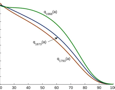
The life expectancies of twenty-year-old males that the model is matched to are given in Figure 4. The data shows that the life expectancy of a twenty-year-old male in 1790 was similar to that of a twenty-year-old male in 1850 and life expectancies fell dramatically for U.S. males (surprisingly also for females) during the antebellum period. In addition, it wasn’t until the twentieth century that mortality conditions in the U.S. began to consistently improve. The data is top-cut at age 100 hence it is assumed that agents live to a maximum age of 80 in the model, i.e. T = 80 for all cohorts. The survival functions of the 1793 cohort, the 1873 cohort and the 1968 cohort are given in Figure 5. The significant reduction in the probability of death at younger ages for the 1968 cohort versus both the 1793 cohort and the 1873 cohort is captured by the rounding out of the survival functions.
14 The exact source for the 1900 to 2000 period is the “United States Life Tables, 2001” inNational Vital Statistics
Reports, Vol. 52, No. 14 (2004).
15 Specifically, for each decade from 1790 to 1840 the survival function is determined by shifting the 1850 survival
function to match the decade-specific life expectancy, i.e., for lack of a better assumption, the survival functions for cohorts born between 1790 and 1850 are assumed to have the same shape as the 1850 survival function.
20 30 40 50 60 70 80 90 100 0 0.1 0.2 0.3 0.4 0.5 0.6 0.7 0.8 0.9 1 Age
Survival Probability q1793(a)
q
1968(a)
q1873(a)
Figure 5: Survival functions of the 1973 cohort, 1848 cohort, and 1968 cohort.
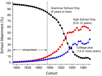
Education Distributions The cohort-specific distributions of agents across education groups, Fτ(e), are calibrated using U.S. Census data on years of school completed by age for males. Since the data is only available every 10 years starting in 1940, the distributions are set as follows. For the 1923 through 1998 cohorts, each distribution is chosen to match that cohort’s corresponding distribution when it is either 30 to 34 years of age or 35 to 39 years of age from the data. For the 1888 to 1918 cohorts, each distribution is set to that cohort’s distribution in 1940 in the data. Finally, for the 1793 to 1883 cohorts, the distributions are determined as follows. First, assume that the fraction of males completing high school grew at a constant rate and the fraction of males completing grammar school fell at a constant rate across the 1793 to 1928 cohorts. Then compute the trendline using the 1888 to 1928 data. Finally, the fractions completing only high school and grammar school are found by extending the trendline back to 1793. The cohort-specific distributions of agents across education groups are summarized in Figure 6.
Market Productivity Profiles and Distributions The market productivity profile of an agent of type sis assumed to be hump-shaped: it reaches its peak height ˜xs when he is age ˜as. From the agent’s expected age of survival, ¯Ts, to the maximum age that can be achieved,T, the
1800 1830 1860 1890 1920 1950 1980 0 10 20 30 40 50 60 70 80 90 100 S ch o o l A t t a i n m e n t ( % ) Cohort
High School Only (9 to 12 years)
College plus (13 or more years) extrapolated
Grammar School Only (8 years or less)
Figure 6: Distributions of agents across education groups by cohort under baseline calibration.
agent’s productivity declines at the constant rate ρs. Thus the agent’s profile is given by
xs(a) = νs(a−˜as)2+ ˜xs, 0≤a≤T¯s, Ωse−ρsa, T¯s< a≤T. (4.12)
Note that an agent’s profile depends on his cohort-specific life expectancy, ¯Ts. Figure 4 provides the sequence of life-expectancies under the baseline calibration.
Determining the market productivity profiles and the distributions of agents of each education type across initial productivity levels requires setting, for each education groupe, the means and standard deviations of the lognormal distributions over initial productivity levels,µeandσe, and, for each type s, the profile parameters ˜as, ˜xs,νs, Ωs, andρs. These parameters are determined simultaneously such that the model matches a set of statistics computed from data. The data used is cross-sectional data on the labor earnings of year-round, full-time male workers in 1975 by years of education from the U.S. Census.16 Of course, the profiles computed from the data
are a proxy for productivity conditional on working. To mitigate the effect of this discrepancy,
16 The specific source is U.S. Bureau of the Census, Current Population Reports, Series P-60, No. 105 ”Money
Income in 1975 of Families and Persons in the United States,” U.S. Government Printing Office, Washington, D.C., 1977. Fuster, Imrohoroglu and Imrohoroglu (2007) also use cross-sectional earnings data for full-time workers by education group as proxies for education-specific productivity profiles. The average profile is similar to that estimated by Hansen (1993) and commonly used in the literature.
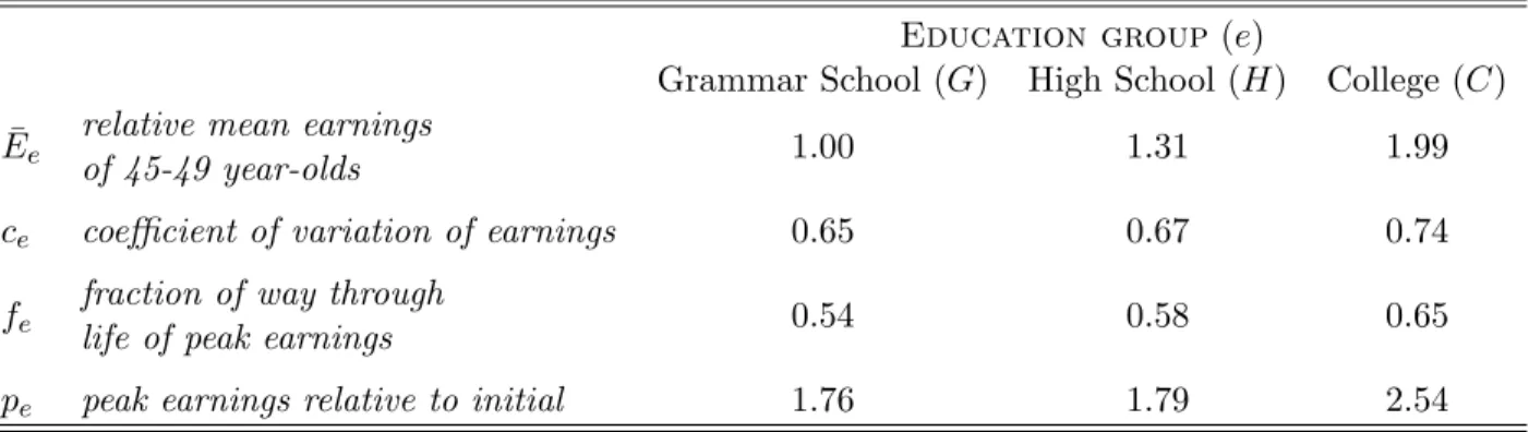
Table 3: Earnings statistics from U.S Census data targeted to calibrate baseline market produc-tivity profiles and initial producproduc-tivity distributions.
Education group(e)
Grammar School (G) High School (H) College (C) ¯
Ee relative mean earningsof 45-49 year-olds 1.00 1.31 1.99
ce coefficient of variation of earnings 0.65 0.67 0.74
fe fraction of way through 0.54 0.58 0.65
life of peak earnings
pe peak earnings relative to initial 1.76 1.79 2.54
the target statistics are based on the earnings of men aged 25 to 55. Profiles are not constructed for each individual cohort because data on earnings by age and education level is unavailable for earlier years.
The statistics computed from the data and matched by the model are: (i) mean earnings of 45 to 49 year-old males with 9 to 12 years of education (high school) relative to those with 8 or less (grammar school), denoted ¯EH; (ii) mean earnings of 45 to 49 year-old males with 13 or more years of education (college) relative to those with 8 or less, denoted ¯EC; (iii) the average coefficient of variation of earnings over the life-cycle by education group, denotedce; (iv) the fraction of the way through expected adult life at which earnings peak by education group, denotedfe; and (v) the ratio of peak earnings to initial earnings by education group, denotedpe. Table 3 shows the target values. Notice that, on average, the earnings of individuals with more education peak later in their life and reach a higher level relative to their initial earnings.
Given these statistics from the data, the parameters are determined as follows. Mean initial log productivity of the grammar school group is normalized to one. The means for the high school and college groups and the standard deviations of initial log productivity are chosen such that the mean (across agents and generations) productivity of agents at age 47 in the high school (college) group relative to the grammar school group is equal to ¯EH ( ¯EC), and for each education groupe, the average (over the life-cycle and across generations) coefficient of variation of productivity is equal toce. The fraction of the way through adult-life at which productivity peaks is assumed to be constant across agents of the same education level regardless of the generation to which they
belong. Thus, for each education group e, ˜as is given by
˜
as=feT¯s.
The ratio of peak earnings to initial earnings is assumed to be constant across agents of the same education level. However, since earlier generations work fewer years before their productivity peaks, the ratio is not assumed to be constant across generations. Instead, thepe’s are only used to determine the ratios for the youngest cohort in the economy, the 1968 cohort. For each type s agent born in 1968 with education level e and initial productivity x0, peak earnings ˜xs is set such that
˜ xs x0 =pe,
and νs is set such that
xs(0) =x0.
For each agent born before 1968 of type ˆs,νˆs is set such that
x0ˆs(0) =x0s(0),
where types ˆsand shave the same education and initial productivity level and ˜xˆsis set such that
xˆs(0) =x0.
In other words, agents with the same education and initial productivity level are assumed to have the same initial slope. This assumption together with the restriction that initial productivity must be given by x0 pins down νs and ˜xs for all the cohorts born before 1968. Finally for each type s agent, Ωs and ρs are calculated by forcing the productivity profiles to be smooth and continuous at ¯Ts, i.e., such that
νs( ¯Ts−˜as)2+ ˜xs= Ωse−ρsT¯s,
and
1900 1920 1940 1960 1980 2000 0.4 0.6 0.8 1 1.2 1.4 1.6 1.8 2 19000 1920 1940 1960 1980 2000 0.5 1 1.5 2 2.5 3 3.5 4 4.5 Year Earnings Index grammar school high school college grammar school high school college
Life Expectancy = 62 Life Expectancy = 69
80 age
20
Figure 7: Sixty-year productivity and earnings profiles of agents from the 1903 and 1943 cohort with the fifth highest initial productivity levels within their education group. Peak productivity and peak earnings of the 1903 grammar school agent are normalized to 1.
The left-hand panel of Figure 7 shows the productivity profiles of agents from the 1903 and 1943 cohort with the fifth highest initial productivity level within each education group. Multiplying the productivity profiles by wages and hours gives the agents’ earnings profiles which are shown in the right-hand panel. Note that, due to wage growth, earnings peak later than productivity. Also, note that the profiles of agents in higher education groups are steeper.
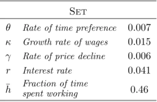
Additional Parameters Five additional parameters that were determined directly from the data are summarized in Table 4. The rate of time preference,θis set such that the average value of θ+η equals 0.02, or in other words, the average annual discount factor is 0.98. The annual growth rate of wages of 1.5 percent is for the period 1830 to 2000. It was determined using the real wage index of Williamson (1995) for the period 1830 to 1988 and BLS data for the period 1988 to 2000. Similarly, the rate at which the price of leisure goods falls is estimated from the leisure price series presented in Figure 3. The 4.1 percent annual interest rate is an after-tax rate and is taken from McGrattan and Prescott (2000). The fraction of time spent working is set to 46 percent. This is the average time spent working of males in the United States over the period 1830 to 2000.17
17 Data on weekly hours worked by U.S. males is from Whaples (1990) and the Statistical Abstracts of the United
Table 4: Parameter values under baseline calibration determined directly from data.
Set
θ Rate of time preference 0.007 κ Growth rate of wages 0.015 γ Rate of price decline 0.006 r Interest rate 0.041 ¯
h Fraction of timespent working 0.46
4.2.2 Estimation
The rest of the parameters are chosen such that the model matches the data along eight moments. The first six moments are the retirement rates of the six cohorts alive in the year 2000.18 The
empirical retirement rates were computed using data from the 2000 HRS and are reported in Table 5. The year 2000 retirement rates are similar to those shown in Section 2.1 found using IPUMS data. The seventh moment is the median drop in market consumption. The target is taken from Hurd and Rohwedder (2008) who find a median drop for individuals of 5.9 percent of pre-retirement expenditure. Their estimate of the consumption drop is the first one based on observations of total expenditure of individuals before and after retirement. The eighth moment is leisure goods’ share of total expenditure in 2000. The empirical value is set to 11.8 percent which is the share of total expenditure allocated to leisure goods according to the BLS and Lebergott (1996) plus 30 percent of transportation’s expenditure share. Both the consumption drop at retirement and leisure goods’ share of total expenditure are discussed in more detail in Section 2.2.
The minimization is done as follows. Assign the numbers 1 through 6 to the six cohorts who are between the ages of 52 and 77 in the year 2000, respectively. Then define the following vector of unknown parameters:
δ= (ˆc, α, ζ, χ, σ, µz, σz, pg,1793).
Given δ, the model’s prediction for the labor force participation rate of cohort i is denoted by
18 The retirement rate is defined in Section 2. The retirement rates for the six cohorts were computed following
Table 5: Moments: Model and Data.
Cohort Year when Age 20 Age in 2000 % Retired in 2000
Data Model 1 1941-45 75-79 82.9 83.5 2 1945-50 70-74 75.6 76.6 3 1951-55 65-69 63.9 65.4 4 1956-60 60-64 38.4 43.9 5 1961-65 55-59 16.7 12.7 6 1966-70 50-54 7.5 0
Median Consumption Drop 5.9 5.9
Leisure Share 11.8 15.9
Pi(δ), the model’s prediction for the median drop in market consumption is denoted by D(δ), and the model’s prediction for leisure goods’ share of total expenditure is denoted by L(δ). The corresponding values in the data are denoted by d, pi, and l, respectively. The exercise now consists of two steps: First, δ is chosen to minimize the sum of the deviations between the model’s output and the empirical moments. Formally,
ˆ δ= arg min δ ( (d−D(δ))2+ (l−L(δ))2+ 6 X i=1 (pi−Pi(δ))2 ) .
Second, the model’s predictions,D(ˆδ), L(ˆδ) and Pi(ˆδ), fori= 1, . . . ,6,are computed using ˆδ.
The results of the minimization are shown in Table 5. Even though there are eight moments and eight parameters the model is unable to match the moments perfectly. Still, the model is able to generate the dispersion in retirement rates across age groups observed in the data.
Notice that the model has more difficulty matching the retirement rates of the younger age groups than the older ones. For example, in the model 43.9 percent of 60 to 64 year-olds are retired in 2000 compared with 38.4 percent in the data. The overestimation of the retirement rates of 60 to 64 year-olds by the model may occur because the model does not account for the impact of Social Security on retirement. As documented in Gustman and Steinmeier (2005), the hazard rate for retirement spikes at ages 62 and 65 in the U.S. These are the ages at which U.S. workers first become eligible for Social Security benefits and can receive benefits without an early retirement reduction penalty, respectively. The hazard rates suggest that individuals may delay or
advance their retirement in order to retire at these particular ages. If there are additional benefits to retiring at ages 62 and 65 not taken into account in the model, the individuals that would most likely adjust their retirement are those with the smallest cost, i.e., those whose optimal retirement age without Social Security is close to either age 62 or age 65. While the impact of delaying or advancing retirement to age 62 on the model’s predictions should be small since individuals aged 60 to 64 are lumped together, the impact of the spike at 65 will not be. If some HRS respondents who, in a world without Social Security, would have chosen to retire at ages close to 65 delayed their retirement to avoid the early retirement reduction penalty, then retirement rates from the model would overestimate those observed in the data for the 60 to 64 year-olds.
The model underestimates the retirement rates of the 55 to 59 year-olds and the 50 to 54 year-olds. In particular, in the model no 50 to 54 year-olds are retired, while 7.5 percent of them are retired in the data. One possible reason for the underestimation is that the model abstracts from intra-generational heterogeneity in life expectancies. In the data life expectancy is positively correlated with income. For example De Nardi, French and Jones (2006) find a 3 year differential in the life expectancies of men in the 20th income percentile compared to men in the 80th at age 70. If this variation in life expectancies was incorporated into the model it would lower the retirement age of low productivity types. The model’s difficulty in matching the retirement rates of the younger age groups may also be due to the fact that retirement before age 60 is more likely to be due to medical conditions that make continuing to work difficult. In addition, starting in 1950, workers with medical conditions who retired were eligible for Social Security Disability Insurance (SSDI) benefits. Poor health combined with SSDI may have provided additional incentives to retire early that are not captured in the model.
The model is able to generate the median consumption drop at retirement observed in the data. However, leisure goods’ share of expenditure in the model (15.9 percent) is larger than the share targeted in the data (11.8 percent). This may be due to the functional form chosen for utility. The assumption that momentary utility is a Cobb-Douglas of market consumption net of subsistence and leisure forces market consumption net of subsistence and non-market time to have the same degree of complimentarily as market consumption net of subsistence and leisure good consumption. Relaxing this assumption could improve the model’s ability to match this target however at a cost of additional complexity. On the other hand, 15.8 is not implausible
Table 6: Parameter values used in baseline model that were chosen to match the model to moments based on data from the 2000 HRS.
Calibrated in Minimization
ˆ
c Subsistence consumption level 0.042∗
α Market consumption’s shareof total consumption 0.33
ξ Weight on leisure goods inleisure production function 0.073
χ Determines elasticity of substitutionbetween leisure goods and leisure time −1.72 σ Determines intertemporal
1.32 elasticity of substitution
µz mean of log leisureproductivity distribution 0.77
σz Std. dev. of log leisureproductivity distribution 1.89 pg,1793 1793 price of leisure goods 8.75
∗Relative to mean annual income of 30-34 year-olds in 1963.
when one considers that there are many leisure expenditures which have not been included in the set of leisure goods given by the BLS. One such example is vacation spending which was 4.2 percent of total expenditure by individuals aged 65 to 74 in 1993.
The values of the parameters that were chosen through the minimization procedure are given in Table 6. The subsistence consumption level is equivalent to approximately 5 dollars a day in year 2000. Note that the values forαandσ imply that the intertemporal elasticity of substitution for market consumption net of subsistence is 0.81.This value is well within the range suggested in the literature.19 The baseline calibration is also consistent with the finding of Weagley and
Huh (2004) discussed in Section 2.2.1 as the increase in leisure time that occurs at the moment of retirement generates an contemporaneous jump in expenditure on leisure goods.
Figure 8 shows the profiles of mean and median wealth over the life cycle for each education group from the 1943 cohort. Consistent with U.S. data the profiles are hump-shaped and peak at the common retirement age of 65. Notice that individuals in higher education groups are wealthier on average. This is consistent with Survey of Consumer Finance (SCF) and Panel
19 For example Attanasio and Weber (1993) find that the IES of consumption should be in the range from 0.3 to
0.8 based on micro data while values as high as 1 are common in real business cycle literature. See Guvenen
20 40 60 80 0.0 0.2 0.4 0.6 0.8 1.0 20 40 60 80 0.0 0.2 0.4 0.6 0.8 1.0 20 40 60 80 0.0 0.2 0.4 0.6 0.8 1.0 m ean m ean m edian m edian m edian W e a l t h I n d e x Age m ean W e a l t h I n d e x Age college W e a l t h I n d e x Age grammar school high school
Figure 8: Life cycle profiles of mean and median wealth by education group in the model.
Study of Income Dynamics data as documented by Cagetti (2003). In addition, the mean profile is above the median illustrating that wealth is skewed across individuals in the same cohort. Aggregating across education groups, the ratio of the mean to median profile at the point when the profiles peak is 1.4. Fern´andez-Villaverde and Krueger (2005) find using cross-sectional data from the SCF that this ratio is about 4 for U.S household in 1995. Thus there is significantly less wealth inequality in the model than in the data. However, this is not surprising given that the model abstracts from many mechanisms that have been shown to be important drivers of wealth inequality in the data such as the social security program, means-tested social insurance programs, and income, medical expense, and survival risk.
4.3 Evolution of Retirement
The model’s prediction for the trend in retirement was obtained by running the calibrated model over the time period from 1793 to 2000. The results are presented in Figure 9. The model predicts that the retirement rates of the age groups above 60 increased steadily over the 150 years. In the data the retirement rate of men aged 75 to 79 goes from approximately 22 percent in 1850 to 85 percent in 2000, an increase of 62 percentage points. In the model the rate is 23 percent in 1850 and 84 percent in 2000, an increase of 60 percentage points. Thus the model captures 96 percent of the increase in retirement of this cohort. By making a similar calculation, the model explains