Querying ontologies in relational database systems

Querying ontologies in relational database systems

Humboldt-Universit¨at zu Berlin, Institute of Computer Sciences, D-10099 Berlin, Germany {trissl, leser}@informatik.hu-berlin.de

Abstract. In many areas of life science, such as biology and medicine, ontolo-gies are nowadays commonly used to annotate objects of interest, such as biolog-ical samples, clinbiolog-ical pictures, or species in a standardized way. In these appli-cations, an ontology is merely a structured vocabulary in the form of a tree or a directed acyclic graph of concepts. Typically, ontologies are stored together with the data they annotate in relational databases. Querying such annotations must obey the special semantics encoded in the structure of the ontology, i.e. relation-ships between terms, which is not possible using standard SQL alone.

In this paper, we develop a new method for querying DAGs using a pre-computed index structure. Our new indexing method extends the pre-/ postorder ranking scheme, which has been studied intensively for trees, to DAGs. Using typical queries on ontologies, we compare our approach to two other commonly used methods, i.e., a recursive database function and the pre-computation of the tran-sitive closure of a DAG.

We show that pcomputed indexes are an order of magnitude faster than re-cursive methods. Clearly, our new scheme is slower than usage of the transitive closure, but requires only a fraction of the space and is therefore applicable even for very large ontologies with more than 200,000 concepts.

1

Introduction

Ontologies play an important role in biology, medicine, and environmental science. The probably oldest ontology in biology is the taxonomic classification of flora and fauna. The NCBI taxonomy [1] is represented as rooted, directed tree, where nodes represent organisms or families, while edges represent an evolutionary relationship between two nodes.

In the area of medicine and molecular biology several ontologies were introduced in the last years, including the Gene Ontology (GO) [2]. The project aims at providing a structured, precisely defined, commonly used, and controlled vocabulary for describing the roles of genes and gene products in any organism. In contrast to the NCBI taxonomy, which resembles a tree, the Gene Ontology is structured in the form of a rooted directed acyclic graph (DAG). Each GO term represents a labeled node in the graph, while an edge represents a direct relationship between two terms.

Ontologies as those mentioned before are used to annotate biological and environ-mental samples, or to define functional characteristic of genes and gene products. Both, the annotated data and the ontologies are stored in information systems, usually in re-lational database systems. Clearly, these data are not just stored, but also queried to answer biologically interesting questions and to find correlations between data items.

The main advantage of ontologies lies in their hierarchical structure. When a query asks for all samples annotated with a certain concept, not only the term itself needs to be considered, but also all its child, grand-child, etc. concepts. Consider the question ”Is the concept transcription factor activity defined as a kind of nucleic acid binding in the Gene Ontology?”.

1.1 Motivation

Graph structures are usually stored using two tables, one for nodes and one for edges. Each edge represents a binary relationship between two nodes, i.e., a father and a child concept. Using this model, it is easy to get parents or children of a node, but not an-cestors or successors as these are in arbitrary distance of the start node. Answering this simple question above using standard SQL alone is therefore impossible.

Generally, there are two different approaches for answering the question. The sim-plest method is to program a recursive function – either as stored procedure or using a host language – that traverses the ontology at run time to compute the answer to the query. However, a recursive functions requires time proportional to the number of tra-versed nodes in the tree or the DAG, leading to bad runtime performance. The second possibility is to index the graph in some way. For instance, one could compute and store the transitive closure of a tree or DAG before queries are posed. Then, a question as the one above can be answered in almost constant time by a simple table lookup. But in-dex structures require time for computation and space for being stored, rendering them inapplicable for very large ontologies.

In this paper we present a new index structure for DAG-formed ontologies that is an order of magnitude faster than recursive functions and in most situations consumes an order of magnitude less space than a pre-computed transitive closure.

The rest of the paper is organized as follows. Section 2 describes our model of stor-ing ontologies, defines typical queries for ontologies, and describes how these queries can be answered using recursive functions. Section 3 describes two well-known index-ing schemes for tree structures, i.e., pre-/ postorder ranks and transitive closure. Section 4 describes how these indexing structures can be extended to index DAGs. The ex-tension of the pre-/ postorder ranking to DAGs is the main contribution of the paper. Section 5 shows our results on implementing and benchmarking the different methods. Finally, Section 6 concludes the paper.

2

Storing and Querying Ontologies

In this section we first describe our model of storing graphs in relational database sys-tems and we then introduce and specify common questions on ontologies. We demon-strate how these data can be queried using recursive database functions. In the next section we then present index structures and how to query them.

2.1 Data model

We consider ontologies that are rooted, directed trees or DAGs. In both structures, a path is a sequence of nodes that are connected by directed edges. The length of a path

is the number of nodes it contains. The length of the shortest path between two nodes is called the distance between the nodes. In a tree each node can be reached on exactly one path from the root node. The same is true for any other two nodes in a directed tree, if a path between the two nodes exists. DAGs are a simple generalization of trees, as nodes may have more than one parent. Therefore, nodes may be connected by more than one path.

In any directed graph successors of a nodevare all nodeswfor which a path fromv

towexists. The successor set ofvare all nodeswthat can be reached fromv. In analogy ancestors of nodevare all nodesuwhere a path fromutovexists. The ancestor set of

vare all nodesufrom whichvcan be reached.

Graphs are stored as a collection of nodes and edges. The information on nodes includes a unique identifier and possibly additional textual annotation. Information on edges is stored as binary relationship between two nodes. Additional attributes on edges can be stored as well. In a relational database system both collections are stored in separate tables. The NODE-table contains all node information including the unique identifier,node name. The second table is calledEDGE, where the binary relationship between two nodes is stored in the attributesfrom nodeandto node.

2.2 Typical queries on ontologies

The main questions on taxonomies and ontologies can be grouped into three categories, namely reachability, ancestor- or successor set, and least common ancestor of two or more nodes.

Q1: Reachability is concerned with questions like ’Does the species Nostoc linckia belong to the phylum Cyanobacteria?’. To answer the question, one has to find out, if the node labeled ’Nostoc linckia’ has an ancestor node labeled ’Cyanobacteria’ in the NCBI taxonomy. The length of the path between the two nodes does not matter.

Q2: Ancestor-/ Successor set of a given node contains all ancestor and succes-sor nodes, respectively. Given a set of proteins, annotated by Gene Ontology terms, a researcher may want to find all proteins that are involved in nucleic acid binding. Of course, not only the proteins directly annotated by the term ’nucleic acid binding’ are of interest, but also all proteins that have a successor term of the original term as anno-tation. The first step in answering the question is to retrieve all successor nodes of the given start term – in short the successor set.

Q3: Least common ancestor is of interest when a common origin of a set of nodes should be computed. For instance, microarray experiments produce expression levels of thousands of different genes within a single experiment. A typical analysis is the clus-tering of genes by the expression levels. A biologist now wants to find commonalities among genes in a cluster. In this situation, GO annotations of genes are helpful, as the least common ancestors of the annotated GO terms defines the most specific common description of the genes in the cluster. Note that for computing the least common an-cestor of a set of nodes, the lengths of the paths between nodes is crucial. Anan-cestor sets of nodes may have several nodes in common, and one has to decide which of these is the closest to all given nodes. Obviously, for answering this question it suffices to know the distance between the nodes.

2.3 Querying Ontologies

The conventional way is to use recursion to traverse a tree or graph on query time. Algorithm 1 performs a depth-first search over a tree and returns the successor set for a node v. The function first looks for children of the start node v and appends each child,mto the successor set. It then searches for successors ofmby calling itself with nodemas the new start node. Doing so, it also holds a counter for the length of the pathvand the current node. As in trees only one path between any two nodes exists, this is equivalent to the distance. As soon as no more child nodes are found the by then accumulated successor set is returned.

Algorithm 1 Recursive Algorithm to retrieve the successor set of a nodev.

FUNCTION successorSet(v, dist) RETURNS succcessors

BEGIN

FOR EACH m∈σf rom node=vEDGEDO

append (m,1) to successors;

successorList(m) := successorSet(m, dist+1);

append successorList(m) to successors;

END FOR; return successors; END;

To compute the ancestor set of a node a second function has to be created, called ancestorSet(). This function takes the same parameters as the one presented in Algorithm 1, but instead of looking for child nodes the algorithm will look for all parent nodes and append them to an ancestor set, which will be returned at the end.

Using these stored procedures, it is possible to query tree and DAG structures. How-ever, for DAGs the function is not optimal. Using the functions the exemplary questions presented in Section 2.2 can be answered with the following SQL statements:

– Q1: Reachability SELECT 1 FROM successorSet(v, 0) WHERE suc = w; – Q2: Ancestor/Successor set SELECT suc FROM successorSet(v, 0);

– Q3: Least common ancestor SELECT A.anc,

A.dist+B.dist AS dist FROM (SELECT anc, dist

FROM ancestorSet(s)) A INNER JOIN (SELECT anc, dist

FROM ancestorSet(t)) B ON A.anc = B.anc

ORDER BY dist;

3

Indexing and querying tree structures

We now show how to index and query tree structures using the pre- and postorder rank-ing scheme as well as the transitive closure.

3.1 Pre- and Postorder ranks

The pre- and postorder rank indexing is well studied for trees [3]. Several systems sug-gested to use it for indexing XML documents in relational databases [4]. The advantage of pre- and postorder rank indexing for an XML document is that the document order is maintained, i.e., the user is able to query for descendant nodes as well as for following. Note that in our case only descending and ascending nodes are of interest, as ontolo-gies usually do not contain any order among children of a node. In chapter 4, we will extend the pre-/ postorder ranking scheme to DAGs. Therefore, we describe the method in detail in the following.

Algorithm 2 shows the function for assigning pre- and postorder ranks to a node in a tree. Ranks are assigned during a depth-first traversal starting at the root node. The preorder rank for a node is assigned as soon as this node is encountered during the traversal. The postorder rank of a node is assigned before any of the ancestor nodes and after all successor nodes have received a postorder rank. We store pre- and postorder ranks together with the node ID in a separate table forming the index. Clearly, the space requirement of the ranks is proportional to the number of nodes in the tree.

Algorithm 2 Pre-/postorder rank assingments of nodes, starting with root noder. var pr:=0; var post:=0;

FUNCTION prePostOrder(r)

BEGIN

FOR EACH child, m∈σf rom node=rEDGEDO

pre:=pr; pr:=pr+1; prePostOrder(m);

INSERT m, pre, post, pr-pre INTO prePostOrder; post:=post+1;

END FOR; END;

To illustrate the steps of the algorithm consider the tree in Figure 1(a). Starting at the root nodeA, we traverse the tree in depth-first order. NodeBgets the preorder rank of 1, whileEgets 2. As nodeE has no further child nodes it is the first node to get a postorder rank and is stored with both ranks in tableprePostOrder. This way the rest of the tree is traversed. The pre- and postorder rank of root nodeA is assigned separately.

In addition to the ranks, we also store the number of descendants,sfor each node, which we will use later for improving queries. This number can be computed as the difference between the current preorder rank and the preorder rank of the node to be inserted next. To clarify this, consider nodeCin Figure 1(a). This node is inserted with the preorder rank of 3. The current preorder rank is 6 as the last successor node ofC,

I has this preorder rank. The difference between the two preorder ranks is 3, which is exactly the number of successor nodes ofC.

Pre- and postorder ranking becomes clearer when it is plotted in a two dimensional co-ordinate plane, with the preorder rank on the x-axis and postorder rank on the y-axis as shown in Figure 1(b).

A B C D E F G H I (a) Tree -6 pre post 4 8 4 8 p p p p p p p p p p p p p p p p p p p p p p p p p p p p p p p p p p p p p p p p p p p p p p p p p p p p p p p p p p p p p p p p p p p p p p p p p p p p p p p p p p p p p p p p p p p p p p p p p p p p p p p p p p p p p p p p p p p p p p p p p p p p p p p p p p p p p p p p p p p p p p p p p p p p p p p p p p p p p p p p p p p p p p p p p p p •A •B • E •A •C • F •C •G • I •A •D •H preceeding ancestor following successor (b) Pre-/Postorder plane of the tree

Fig. 1. Pre-/postorder rank assignment of a tree

Querying pre-/postorder indexed trees. As indicated for nodeGin Figure 1(b) the pre-post plane can be partitioned into four disjoint regions for each nodev. The upper-left partition contains all ancestors ofv, while the successors can be found in the lower-right area. The remaining two areas hold the preceeding and following nodes ofv.

As ontological structures are usually order-independent, only the ancestor and suc-cessor sector are of interest. Using the preassigned ranks, nodes in these two partitions can be retrieved without recursion, since any successor of nodevmust have a preorder rank that is higher and a postorder rank that is lower than that of v. The location of the successors of a nodevwithin the lower-right partition can be further restricted. Let nodevhave preorder rankprev. Ifvhasssuccessor nodes, then each successorwof nodevwill have a preorder rankprewwithprev< prew≤prev+s.

To find the least common ancestor of two nodes the ancestor sets of both nodes have to be joined on the attributenode nameand the common ancestor with the highest preorder rank is least common ancestor of both nodes.

Using the refinement on the location of the successors the queries for answering questions Q1, Q2, and Q3 are the following:

– Q1: Reachability(iswsuccessor ofv) SELECT 1

FROM prePostOrder p1, prePostOrder p2 WHERE p1.node name = w

AND p2.node name = v AND p1.pre > p2.pre AND p1.pre ≤ p2.pre+p2.s; – Q2: Ancestor set

SELECT p1.node name AS u FROM prePostOrder p1,

prePostOrder p2 WHERE p2.node name = v

AND p1.pre < p2.pre AND p1.post > p2.post;

– Q2: Successor set

SELECT p1.node name AS w FROM prePostOrder p1

prePostOrder p2 WHERE p2.node name = v

ANDp1.pre > p2.pre

– Q3: Least common ancestor SELECT A.node name, A.pre FROM (

SELECT p1.node name, p1.pre FROM prePostOrder p1,

prePostOrder p2 WHERE p2.node name = s

AND p1.pre < p2.pre AND p1.post > p2.post) A

INNER JOIN (

SELECT p1.node name, p1.pre FROM prePostOrder p1,

prePostOrder p2 WHERE p2.node name = t

AND p1.pre < p2.pre AND p1.post > p2.post) B ON A.node name = B.node name ORDER BY A.pre desc;

3.2 Transitive closure

The transitive closure of a graph is a set of edges. Edge (v,w) is inserted into the transi-tive closure if either (v,w) is an edge in the graph or if there exists a path between node

vandw. Using the transitive closure, queries on reachability and queries for ancestor and successor sets can be answered very efficiently. Finding the least common ances-tor of two or more nodes requires to sances-tore the length of the shortest path between two nodes.

In the past, several algorithms have been developed to compute the transitive clo-sure within a relational database system [5]. We found that the so called ’Logarithmic algorithm’ [6] performed best for trees as well as DAGs. The function is presented in Algorithm 3.

Algorithm 3 Computing the transitive closure. FUNCTION transtiveClosure()

BEGIN

INSERT INTO TC SELECT from node, to node, 1 FROM EDGE; max dist:=1;

REPEAT

INSERT INTO TC SELECT TC1.anc, TC2.suc, min(TC1.dist+TC2.dist) FROM TC TC1, TC TC2 WHERE TC1.suc=TC2.anc AND TC1.dist=max dist; max dist:= SELECT max(dist) FROM TC;

UNTIL INSERT=∅

END;

This algorithm first inserts all tuples of the initial edge relation with the distance 1 to the transitive closure tableTC. In the next step the tuples fromTCwith a distance equal to the maximum distance are self-joined withTC. The join condition is that the successor node of one relation must be equal to the ancestor node of the other. The ancestor nodes of the first relation, the successor node of the second and the minimal distance between the two nodes is stored inTC. This step is repeated until no further tuples can be inserted intoTC.

Note that the transitive closure requires space that is in worst caseO(|V|2_{). Clearly,} the real space requirements are much smaller for trees, as they are for DAGs. In Section 5, we will measure space consumption of transitive closures in more detail.

Querying the transitive closure. The transitive closure essentially contains one tuple for each pair of ancestor - successor nodes. Accordingly, queries answering our three problems may look as follows:

– Q1: Reachability SELECT 1 FROM TC WHERE anc = v AND suc = w; – Q2: Ancestor/Successor set SELECT suc FROM TC WHERE anc = v;

– Q3: Least common ancestor SELECT A.anc, A.dist+B.dist AS distance

FROM (SELECT anc, dist FROM TC WHERE suc = s) A INNER JOIN (SELECT anc, dist

FROM TC WHERE suc = t) B ON A.anc = B.anc

ORDER BY distance;

4

Extending index structures to DAGs

So far, we only considered trees for querying. In this section we extend the indexing schemes to work on DAGs, as ontologies often have the form of directed acyclic graphs. Specifically, we present how the pre- and postorder ranking scheme can be used for DAGs and how this structure can be queried.

4.1 Pre- and Postorder ranks for DAGs

The pre-/ postorder ranking scheme we described in the previous chapter is restricted to trees. The reason is that in DAGs, where nodes may be reached on more than one path from root, neither the pre- nor the postorder rank is unique for a single node. If multiple paths exist, a node is reached more than once during the traversal.

Obviously, it is no option to simply take any one of the ranks, e.g., the first to be assigned, because then the relationships between the ranks of ancestors and successors do not hold any more. Consequently, we would loose successors or ancestors during querying.

In the following, we describe a new and simple extension of the ranking scheme that is also capable of indexing DAGs. We will show in Section 5 that our method can be seen as a compromise between recursive query methods, which are slow for queries but need no further storage and the transitive closure, which allows for very fast queries, but also requires considerable storage space. We will also show that the advantages of our method depend on the ”tree-likeness” of a DAG. For DAGs that are almost trees, our method has considerable advantages when compared to the transitive closure, however, these advantages are lost the less tree-like a DAG is.

The basic idea of our extension is very simple. Instead of assigning only one pair of ranks to a node, we allow for multiple rank pairs. More specifically we assign an additional pre- and postorder rank to a node each time this node is encountered during the depth-first traversal. Actually, Algorithm 2 already performs this computation, as it inserts a new node-rank combination each time a node is encountered. After running

the function on a DAG, each node will have as many pre- and postorder ranks as this node occurs in a path from the root node.

A

B C D

E F G H

I (a) DAG

node pre post s

A 0 12 12 B 1 1 1 C 3 5 3 D 7 11 5 E 2 0 0 F 4 2 1 G 5 4 1 H 8 10 4 I 6 3 0 C 9 9 3 F 10 6 0 G 11 8 1 I 12 7 0

(b) Table with pre-/ postorder ranks and number of successors

Fig. 2. Pre-/postorder rank assignment of a directed acyclic graph.

As an example, we add one more edge (the dotted edge) to the tree from figure 1(a). Table 2(b) shows the resulting pre- and postorder ranks for each node in the DAG. As one can see nodeCand all descendants ofCget two different rank pairs, because these nodes are encountered on two different paths, one directly fromAtoCand one from

AoverDandHtoC.

Clearly, the number of node-rank pairs is higher for DAGs than for trees, leading to an increase in space consumption for the index. The degree of increase depends on the number of additional non-tree edges and the location of such an edge in the graph. Clearly, additional edges in the upper levels of the tree will lead to an addition of rank pairs for a large number of nodes, while additional edges close to the leaves of a DAG only have marginal impact. Potentially there is an exponential growth of the index structure in the number of edges added. However, we observed that in practice the increase in size is not critical. The reason for this is that in ontologies concepts on the upper level usually only have one parent concept. For instance, in the Gene Ontology the first level where a node has two or more parents is on level four. In Section 5, we will show the impact in size more precisely both on real ontologies and on randomly generated trees and DAGs.

Like for trees, all rank pairs in the DAG can be plotted on a two-dimensional coor-dinate plane (see Figure 3). Nodes appear as many times in the plane as they have rank pairs. This shows that, intuitively, our method multiplies all subtrees of nodes that have more than one parent.

To query our new indexing scheme, we need to adapt the methods for querying pre-post order indexes for trees. As an example, consider nodeGin Figure 3. This node as well as its successor set appears twice in the coordinate plane as it can be reached on two different paths from the root nodeA. However, the successor sets are identical

-6 pre post 4 8 12 4 8 12 p p p p p p p p p p p p p p p p p p p p p p p p p p p p p p p p p p p p p p p p p p p p p p p p p p p p p p p p p p p p p p p p p p p p p p p p p p p p p p p p p p p p p p p p p p p p p p p p p p p p p p p p p p p p p p p p p p p p p p p p p p p p p p p p p p p p p p p p p p p p p p p p p p p p p p p p p p p p p p p p p p p p p p p p p p p p p p p p p p p p p p p p p p p p p p p p p p p p p p p p p p p p p p p p p p p p p p p p p p p p p p p p p p p p p p p p p p p p p p p p p p p p p p p p p p p p p p p p p p p p p p p p p p p p p p p p p p p p p p p p p p p p p p p p p p p p p p p p p p p p p •A •B •E •A •C •F •C •G •I •A •D •H •C •G •I •C •F

Fig. 3. Pre-/postorder plane of a DAG.

for each instance ofG, because this set is independent of the number of pathsGcan be reached from root. Thus, for successor queries it suffices to select any instance of a node and query for all its children using the conditions on pre- and post order rank used for trees. This is reflected by limiting the number of returned preorder ranks in the query to 1. As for trees the search space can be reduced by using the information on the number of descending nodes. However, caution must be taken to filter the result for duplicates.

The situation is more complex for ancestor queries, e.g., the ancestor set of a node

v. Computing this set requires to merge all nodes in the upper-left partition of any instances ofv, as the set of one instance only contains nodes for one possible path from root tov. Again, duplicates must be removed from the result.

– Successor set: SELECT DISTINCT p1.node name AS w FROM prePostOrder p1 WHERE p1.pre > ( SELECT p1.pre FROM prePostOrder p2 WHERE p2.node name = v LIMIT 1)

AND p1.pre ≤ (

SELECT p2.pre+p2.s FROM prePostOrder p2 WHERE p2.node name = v LIMIT 1);

– Ancestor set for DAGs: SELECT DISTINCT

p2.node name AS u FROM prePostOrder p1,

prePostOrder p2 WHERE p1.node name = v AND p2.pre < p1.pre AND p2.post > p1.post;

We only gave the code for computing the successor and the ancestor set. Reacha-bility can be computed in the same way as for trees. Least common ancestor requires to compute the ancestor sets of all nodes, intersect them, and find the node with the minimal sum of the differences between the preorder ranks of the two nodes and the common ancestor node.

4.2 Transitive Closure on DAGs

Algorithm 3 can be applied without changes to index DAGs. The space complexity will not change if only the minimal distance between any two nodes is stored. If all possible path lengths between two nodes are needed, the situation would be different and the upper bound would be exceeded.

Querying the transitve closure of DAGs is the same as for trees.

5

Results

In this section we compare both indexing methods and the recursive algorithm. We measure in detail run time of queries, space consumption of the index structures, and time necessary for building the indexes. We give results on generated tree and DAG structures and on real data, i.e., queries against the Gene Ontology.

We have implemented both indexing algorithms and the recursive algorithm as stored procedures in ORACLE 9i. Tests were performed on a DELL dual Xeon ma-chine with 4 GB RAM. Queries were run without rebooting the database. Given the relative small size of the data being studied (in the range of a couple of megabytes), we expected that all computation is very likely performed solely in main memory, as both data and index blocks can be cached completely. Thus, secondary memory issues were not considered.

5.1 Time and space consumption of graph indexing algorithms

To systematically measure the construction time and space consumption of the two index algorithms we generated trees with a given number of nodes and a given average degree of 8.0. The average degree is the average number of incoming and outgoing edges of a node, therefore in our trees each node has on average 7 children. DAGs were created by randomly adding additional edges to the tree, independent of the depth of the newly connected nodes. Added edges had to fulfill two conditions: First, it was not allowed to introduce parallel edges, and second, no edge between nodev and an ancestor node ofvwas allowed, as this would introduce a cycle. The index structures of the generated trees and DAGs were created using Algorithms 2 and 3.

Figure 4 shows the size of the index structures given as the number of tuples inserted in the index relation. The starting point of a curve always stands for the tree with the indicated number of edges. To create DAGs we have iteratively added additional 10 % of the number of edges from the corresponding tree. For instance, starting with a tree of 10,000 edges, the second measurement contains 11,000, the third 12,000 edges, ect. Thus, in each line all but the first point represent DAGs. Altogether, we used 11 start points of trees with 1,000 to 200,000 nodes, performing 1 to 5 rounds of edge additions. For a tree, the number of tuples inserted intoprePostOrderequals the number of nodes. For most measured cases, the size of the index using our method is an order of magnitude smaller than the size of the transitive closure. However, we see that sizes ofTCandprePostOrderare converging as the number of non-tree edges in a DAG increases. Adding up to 30 % more edges still leads to more than 50 % less tuples in the pre-/postorder index than for transitive closure in any of the examined sets.

Fig. 4. Size of index depending on the size of the tree or DAG, respectively. Black stars give the size forTC, gray boxes forprePostOrder. Note that both axes use logarithmic scale.

However, adding 40 % more edges reverses the situation in two of the shown sets. The reason for this behavior is that, when adding additional edges to the tree, the end node of the added edge plays an important role for the pre- and postorder ranking, but not so much for the transitive closure. Imagine, you have already added a certain amount of additional edges to the tree, and now you add a new edge. The pre-/ postorder ranking now has to traverse another sub-structures more than once, and the nodes within that structure will get an additional rank pair. The transitive closure will also increase, as new connections are established. But the number of newly found connections decreases the more edges already exist in the DAG, as many new edges only introduce new paths between already connected nodes, thus not increasing the size of the transitive closure. We can conclude that our method uses considerably less space than the transitive closure for DAGs that are tree-like. Note that the measurements on a real ontology are even more favorable for our method (see below).

The time required to construct the pre-/ postorder index for trees is always 3 to 10 times higher than for the transitive closure (data not shown). However, the actual time difference is marginal, as both structures can be computed very fast even for large trees. Computing the transitive closure for a tree of 200,000 nodes takes 58 seconds, while the pre-/postorder ranking index needs 3:45 minutes.

The time difference increases quickly with the number of edges added. For up to 20 % more edges, the difference remains within the order of the differences for trees. Adding more edges leads to a dramatic increase in the time necessary for computing the pre-/ postorder index. For a DAG with 10,000 nodes and 13,999 edges, it already takes 71 times more time to compute the pre-/ postorder than the transitive closure, although the number of inserted tuples in both tables is nearly equal. The reason for this differ-ence is that pre-/ postorder ranks require extensive graph traversal, while the transitive closure can be efficiently computed using dynamic programming - style algorithms over increasing path lengths.

5.2 Querying ontologies

We measured query times for three exemplary questions described in Section 2.2, based on real ontologies. We used real ontologies and not generated ones to obtain more re-alistic results, as in human curated ontologies concepts on higher levels usually do not have more than one parent. This specific edge distribution is not included in our DAG generator.

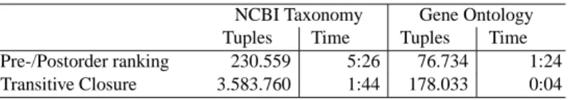
NCBI Taxonomy Gene Ontology Tuples Time Tuples Time Pre-/Postorder ranking 230.559 5:26 76.734 1:24 Transitive Closure 3.583.760 1:44 178.033 0:04

Table 1. Number of tuples inserted in each relation and time (in min:sec) required for computing the index structures.

Table 1 shows for the two ontologies, i.e. the NCBI Taxonomy and the Gene On-tology the size of the index structure and the time required for computing both indexes. As the NCBI Taxonomy is a tree, the pre-/ postorder index is much smaller than the transitive closure. The figures are more interestingly for the Gene Ontology. We used a version with 16.859 nodes and 23.526 edges. Although the number of edges exceeds the number of nodes by approximately 40 %, the size of the pre-/ postorder index is still considerably smaller than the transitive closure, confirming our observation about the edge distribution in real ontologies.

In the following, due to space restrictions, we only give query times for Gene Ontol-ogy. For each of the queries, Q1, Q2, and Q3, 25 % of the nodes of the Gene Ontology were randomly selected. The query for each node was issued 20 times. The following figures give average query execution times.

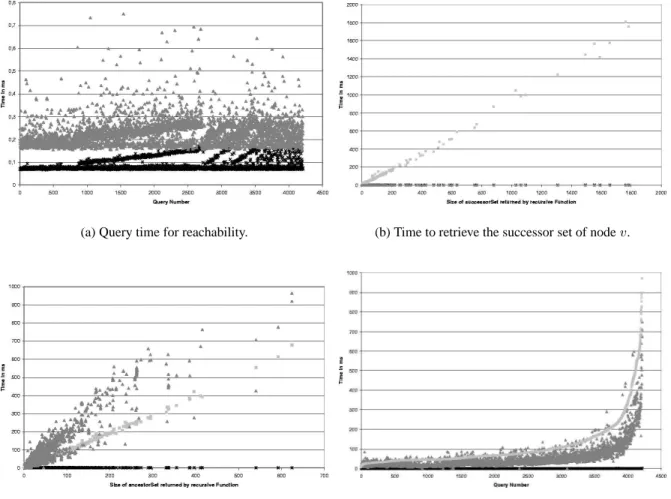
Reachability. We computed times for answering the query ’Is wa successor node ofv?’ for randomly selectedw andv. Figure 5(a) shows the times for 4,300 single queries using either of the two index structures. As one can see, querying the transitive closure is faster than querying the pre-/ postorder index, but only by a small and almost constant factor. The recursive function, whose running time depends on the number of nodes traversed, is not displayed, as it required between 6 and 11,000 times more time than querying the indexing schemes.

Successor Set. The successor set for 25 % randomly selected nodes from the Gene Ontology was retrieved using the queries presented in the former sections. Results can be found in Figure 5(b). Note that the successor set returned from the recursive function and from querying the pre-/ postorder index can contain successor nodes several times. The successor set from the transitive closure will contain any node only once.

Query times using a recursive function is linearly dependent on the number of tu-ples returned. Times for both index structures remain fairly constant over the number of tuples. Times for querying using the pre-/ postorder index are on average 1.5 times higher than using the transitive closure.

Ancestor Set. Figure 5(c) shows the time needed to retrieve ancestor sets. In this case, the indexing methods differ considerably. While query times using transitive closure are

(a) Query time for reachability. (b) Time to retrieve the successor set of nodev.

(c) Time required to compute the ancestor set. (d) Time to get the least common ancestor of two nodes.

Fig. 5. Query times for the three presented methods for the different queries. The light-gray squares are the query times for the recursive function,

similar to the times for the successor set, times for querying the pre-/ postorder index is even more costly than using a recursive function. The reason that the pre-/ postorder index is slow is that the ancestor set has to be calculated for every instance of the start node leading to an extremely redundant ancestor set.

Least Common Ancestor. Computing the least common ancestor of two nodes first requires to compute the ancestor sets of each node, second to find common nodes in both sets, and third to select the node with the minimal distance to both original nodes. Figure 5(d) shows the time necessary to compute the least common ancestor of 4,300 randomly selected pairs of nodes, sorted by the time required for computing the an-swer using the recursive function. The figure shows that querying the pre-/ postorder index structure is better than using a recursive database function and worse than using the transitive closure. The results resemble the one shown in Figure 5(c), as the cost-dominating operation is the computation of the ancestor sets. The steep rise in time for some ”pathological” node pairs, i.e., queries where both sets have extremely large ancestor sets, is somewhat surprising and deserves further study.

6

Discussion

Indexing tree and graph structures is a lively research area. In the XML community the pre-/ postorder ranking scheme is widely used as it preserves information about the document order and allows very fast queries at four axis of the XQuery model. To further optimize access to tree data in relational databases, Mayer et al. [7] have created the so called ’Staircase Join’, a special join operator for queries against pre-/ postorder ranking schemes. It is unclear of this method could also be extended to DAGs.

Vagena et al. [8] presented a different numbering scheme for DAGs. This scheme also conserves the document order, but it is restricted to planar DAGs. As we can not guarantee that every ontology has such a structure, the algorithm is not universally applicable. Another numeric indexing structure for DAGs was presented in [9], where they label spanning trees with numeric intervals. In DAGs not the nodes with several parent nodes get more than one interval, but all ancestor nodes get the first interval of that node. They proposed a reduction, but as intervals are propagated upwards in real ontologies this would probably lead to an index size in the same order of magnitude.

A different indexing method for trees and graphs was proposed by Schenkel et al. [10]. Their method uses the 2-hop cover [11] of a graph, which is more space efficient than the transitive closure and allows to answer reachability queries with a single join. Since computing optimal 2-hop covers is NP hard, they use an approximation optimized for very large XML documents with XPointers. However, 2-hop covers do not allow for least common ancestor queries, as no distance information can be preserved.

[12, 13] are examples of attempts to index graph structures, one by finding and in-dexing all frequent subgraphs, and one by exploiting properties of the network structure. However, both methods are for full graphs, and we would expect them to perform rather poor on DAGs. In the ontology community, we are not aware of any work on optimized indexing and querying of large ontologies.

We have presented a novel structure for indexing and querying large ontologies, extending the well known pre- and postorder ranking scheme to DAGs. Our method has

favorable properties for ontologies that are tree-like, which is true for most ontologies we are aware of. In those cases, most queries for successors are almost as fast as using the transitive closure, while space consumption is an order of magnitude lower. One drawback of our method is the time for creating the index. Our current research is geared towards reducing this time and speed up ancestor queries.

7

Acknowledgement

This work is supported by BMBF grant no. 0312705B (Berlin Center for Genome-Based Bioinformatics).

References

1. DL Wheeler, C Chappey, AE Lash, DD Leipe, TL Madden, GD Schuler, TA Tatusova, and BA Rapp. Database resources of the National Center for Biotechnology Information. Nucleic

Acids Research, 28(1):10 – 14, Jan 2000.

2. Gene Ontoloy Consortium. The Gene Ontology (GO) database and inforamtics resource.

Nucleic Acids Research, 32:D258 – D261, 2004. Database issue.

3. P. Dietz and D. Sleator. Two algorithms for maintaining order in a list. In Proceedings of the

nineteenth annual ACM conference on Theory of computing, pages 365–372. ACM Press,

1987.

4. Torsten Grust. Accelerating XPath location steps. In Proceedings of the 2002 ACM SIGMOD

international conference on Management of data, pages 109–120. ACM Press, 2002.

5. Hongjun Lu. New strategies for computing the transitive closure of a database relation. In

Proceedings of the 13th International Conference on Very Large Data Bases, pages 267–274.

Morgan Kaufmann Publishers Inc., 1987.

6. P. Valduriez and H. Boral. Evaluation of recursive queries using join indices. In L. Ker-schberg, editor, First International Conference on Expert Database Systems, pages 271–293, Redwood City, CA, 1986. Addison-Wesley.

7. Sabine Mayer, Torsten Grust, Maurice van Keulen, and Jens Teubner. An injection of tree awareness: Adding staircase join to postgresql. In Mario A. Nascimento, M. Tamer ¨Ozsu, Donald Kossmann, Ren´ee J. Miller, Jos´e A. Blakeley, and K. Bernhard Schiefer, editors,

VLDB, pages 1305–1308. Morgan Kaufmann, 2004.

8. Zografoula Vagena, Mirella Moura Moro, and Vassilis J. Tsotras. Twig query processing over graph-structured xml data. In Sihem Amer-Yahia and Luis Gravano, editors, WebDB, pages 43–48, 2004.

9. Rakesh Agrawal, Alexander Borgida, and H. V. Jagadish. Efficient management of transitive relationships in large data and knowledge bases. In James Clifford, Bruce G. Lindsay, and David Maier, editors, SIGMOD Conference, pages 253–262. ACM Press, 1989.

10. Ralf Schenkel, Anja Theobald, and Gerhard Weikum. Efficient creation and incremental maintenance of the hopi index for complex xml document collections. In ICDE, 2005. 11. Edith Cohen, Eran Halperin, Haim Kaplan, and Uri Zwick. Reachability and distance queries

via 2-hop labels. SIAM J. Comput., 32(5):1338–1355, 2003.

12. Andrew Y. Wu, Michael Garland, and Jiawei Han. Mining scale-free networks using geodesic clustering. In Won Kim, Ron Kohavi, Johannes Gehrke, and William DuMouchel, editors, KDD, pages 719–724. ACM, 2004.

13. Xifeng Yan, Philip S. Yu, and Jiawei Han. Graph indexing: A frequent structure-based ap-proach. In Gerhard Weikum, Arnd Christian K¨onig, and Stefan Deßloch, editors, SIGMOD