Show and Tell: A Neural Image Caption Generator
Oriol Vinyals
Alexander Toshev
Samy Bengio
Dumitru Erhan
Abstract
Automatically describing the content of an image is a fundamental problem in artificial intelligence that connects computer vision and natural language processing. In this paper, we present a generative model based on a deep re-current architecture that combines recent advances in com-puter vision and machine translation and that can be used to generate natural sentences describing an image. The model is trained to maximize the likelihood of the target de-scription sentence given the training image. Experiments on several datasets show the accuracy of the model and the fluency of the language it learns solely from image descrip-tions. Our model is often quite accurate, which we verify both qualitatively and quantitatively. For instance, while the current state-of-the-art BLEU score (the higher the bet-ter) on the Pascal dataset is 25, our approach yields 59, to be compared to human performance around 69. We also show BLEU score improvements on Flickr30k, from 55 to 66, and on SBU, from 19 to 27.
1. Introduction
Being able to automatically describe the content of an image using properly formed English sentences is a very challenging task, but it could have great impact, for instance by helping visually impaired people better understand the content of images on the web. This task is significantly harder, for example, than the well-studied image classifi-cation or object recognition tasks, which have been a main focus in the computer vision community [26]. Indeed, a description must capture not only the objects contained in an image, but it also must express how these objects relate to each other as well as their attributes and the activities they are involved in. Moreover, the above semantic knowl-edge has to be expressed in a natural language like English, which means that a language model is needed in addition to visual understanding.
Most previous attempts have proposed to stitch together existing solutions of the above sub-problems, in order to go from an image to its description [6, 15]. In contrast, we
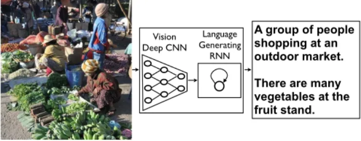
A group of people shopping at an outdoor market. !
There are many vegetables at the fruit stand. Vision! Deep CNN Language ! Generating! RNN
Figure 1. NIC, our model, is based end-to-end on a neural net-work consisting of a vision CNN followed by a language gener-ating RNN. It generates complete sentences in natural language from an input image, as shown on the example above.
would like to present in this work a single joint model that takes an image I as input, and is trained to maximize the likelihoodp(S|I)of producing a target sequence of words
S ={S1, S2, . . .}where each wordStcomes from a given
dictionary, that describes the image adequately.
The main inspiration of our work comes from recent ad-vances in machine translation, where the task is to transform a sentenceSwritten in a source language, into its transla-tionT in the target language, by maximizingp(T|S). For many years, machine translation was also achieved by a se-ries of separate tasks (translating words individually, align-ing words, reorderalign-ing, etc), but recent work has shown that translation can be done in a much simpler way using Re-current Neural Networks (RNNs) [3, 2, 29] and still reach state-of-the-art performance. An “encoder” RNNreadsthe source sentence and transforms it into a rich fixed-length vector representation, which in turn in used as the initial hidden state of a “decoder” RNN thatgeneratesthe target sentence.
Here, we propose to follow this elegant recipe, replac-ing the encoder RNN by a deep convolution neural network (CNN). Over the last few years it has been convincingly shown that CNNs can produce a rich representation of the input image by embedding it to a fixed-length vector, such that this representation can be used for a variety of vision tasks [27]. Hence, it is natural to use a CNN as an image “encoder”, by first pre-training it for an image classification
1
task and using the last hidden layer as an input to the RNN decoder that generates sentences (see Fig. 1). We call this model the Neural Image Caption, or NIC.
Our contributions are as follows. First, we present an end-to-end system for the problem. It is a neural net which is fully trainable using stochastic gradient descent. Second, our model combines state-of-art sub-networks for vision and language models. These can be pre-trained on larger corpora and thus can take advantage of additional data. Fi-nally, it yields significantly better performance compared to state-of-the-art approaches; for instance, on the Pascal dataset, NIC yielded a BLEU score of 59, to be compared to the current state-of-the-art of 25, while human performance reaches 69. On Flickr30k, we improve from 55 to 66, and on SBU, from 19 to 27.
2. Related Work
The problem of generating natural language descriptions from visual data has long been studied in computer vision, but mainly for video [7, 31]. This has led to complex sys-tems composed of visual primitive recognizers combined with a structured formal language, e.g. And-Or Graphs or logic systems, which are further converted to natural lan-guage via rule-based systems. Such systems are heav-ily hand-designed, relatively brittle and have been demon-strated only on limited domains, e.g. traffic scenes or sports. The problem of still image description with natural text has gained interest more recently. Leveraging recent ad-vances in recognition of objects, their attributes and loca-tions, allows us to drive natural language generation sys-tems, though these are limited in their expressivity. Farhadi et al. [6] use detections to infer a triplet of scene elements which is converted to text using templates. Similarly, Li et al. [18] start off with detections and piece together a fi-nal description using phrases containing detected objects and relationships. A more complex graph of detections beyond triplets is used by Kulkani et al. [15], but with template-based text generation. More powerful language models based on language parsing have been used as well [22, 1, 16, 17, 5]. The above approaches have been able to describe images “in the wild”, but they are heavily hand-designed and rigid when it comes to text generation.
A large body of work has addressed the problem of rank-ing descriptions for a given image [11, 8, 23]. Such ap-proaches are based on the idea of co-embedding of images and text in the same vector space. For an image query, de-scriptions are retrieved which lie close to the image in the embedding space. Most closely, neural networks are used to co-embed images and sentences together [28] or even image crops and subsentences [12] but do not attempt to generate novel descriptions. In general, the above approaches cannot describe previously unseen compositions of objects, even though the individual objects might have been observed in
the training data. Moreover, they avoid addressing the prob-lem of evaluating how good a generated description is.
In this work we combine deep convolutional nets for im-age classification [30] with recurrent networks for sequence modeling [10], to create a single network that generates de-scriptions of images. The RNN is trained in the context of this single “end-to-end” network. The model is inspired by recent successes of sequence generation in machine trans-lation [3, 2, 29], with the difference that instead of starting with a sentence, we provide an image processed by a con-volutional net. The closest works are by Kiros et al. [14] who use a neural net, but a feedforward one, to predict the next word given the image and previous words. A recent work by Mao et al. [20] uses a recurrent NN for the same prediction task. This is very similar to the present proposal but there are a number of important differences: we use a more powerful RNN model, and provide the visual input to the RNN model directly, which makes it possible for the RNN to keep track of the objects that have been explained by the text. As a result of these seemingly insignificant dif-ferences, our system achieves substantially better results on the established benchmarks. Lastly, Kiros et al. [13] pro-pose to construct a joint multimodal embedding space by using a powerful computer vision model and an LSTM that encodes text. In contrast to our approach, they use two sepa-rate pathways (one for images, one for text) to define a joint embedding, and, even though they can generate text, their approach is highly tuned for ranking.
3. Model
In this paper, we propose a neural and probabilistic framework to generate descriptions from images. Recent advances in statistical machine translation have shown that, given a powerful sequence model, it is possible to achieve state-of-the-art results by directly maximizing the proba-bility of the correct translation given an input sentence in an “end-to-end” fashion – both for training and inference. These models make use of a recurrent neural network which encodes the variable length input into a fixed dimensional vector, and uses this representation to “decode” it to the de-sired output sentence. Thus, it is natural to use the same ap-proach where, given an image (instead of an input sentence in the source language), one applies the same principle of “translating” it into its description.
Thus, we propose to directly maximize the probability of the correct description given the image by using the follow-ing formulation: θ?= arg max θ X (I,S) logp(S|I;θ) (1)
whereθare the parameters of our model,Iis an image, and
its length is unbounded. Thus, it is common to apply the chain rule to model the joint probability overS0, . . . , SN, whereN is the length of this particular example as
logp(S|I) =
N
X
t=0
logp(St|I, S0, . . . , St−1) (2)
where we dropped the dependency on θ for convenience. At training time, (S, I)is a training example pair, and we optimize the sum of the log probabilities as described in (2) over the whole training set using stochastic gradient descent (further training details are given in Section 4).
It is natural to modelp(St|I, S0, . . . , St−1)with a Re-current Neural Network (RNN), where the variable number of words we condition upon up tot−1is expressed by a fixed length hidden state or memory ht. This memory is updated after seeing a new inputxtby using a non-linear functionf:
ht+1=f(ht, xt). (3) To make the above RNN more concrete two crucial design choices are to be made: what is the exact form of f and how are the images and words fed as inputsxt. Forf we
use a Long-Short Term Memory (LSTM) net, which has shown state-of-the art performance on sequence tasks such as translation. This model is outlined in the next section.
For the representation of images, we use a Convolutional Neural Network (CNN). They have been widely used and studied for image tasks, and are currently state-of-the art for object recognition and detection. Our particular choice of CNN follows the winning entry of the ILSVRC 2014 clas-sification competition [30]. Furthermore, they have been shown to generalize to other tasks such as scene classifi-cation by means of transfer learning [4]. The words are represented with an embedding model.
3.1. LSTM-based Sentence Generator
The choice off in (3) is governed by its ability to deal with vanishing and exploding gradients [10], the most com-mon challenge in designing and training RNNs. To address this challenge, a particular form of recurrent nets, called LSTM, was introduced [10] and applied with great success to translation [3, 29] and sequence generation [9].
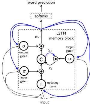
The core of the LSTM model is a memory cellc encod-ing knowledge at every time step of what inputs have been observed up to this step (see Figure 2) . The behavior of the cell is controlled by “gates” – layers which are applied mul-tiplicatively and thus can either keep a value from the gated layer if the gate is1or zero this value if the gate is 0. In particular, three gates are being used which control whether to forget the current cell value (forget gatef), if it should read its input (input gatei) and whether to output the new
h σ σ σ
c
input LSTM memory block word prediction softmax input gate i output gate f forget gate f updating term ct-1 ct mt xFigure 2. LSTM: the memory block contains a cellcwhich is controlled by three gates. In blue we show the recurrent connec-tions – the outputmat timet−1is fed back to the memory at timetvia the three gates; the cell value is fed back via the forget gate; the predicted word at timet−1is fed back in addition to the memory outputmat timetinto the Softmax for word prediction.
cell value (output gateo). The definition of the gates and cell update and output are as follows:
it = σ(Wixxt+Wimmt−1) (4) ft = σ(Wf xxt+Wf mmt−1) (5) ot = σ(Woxxt+Wommt−1) (6) ct = ftct−1+ith(Wcxxt+Wcmmt−1)(7) mt = otct (8) pt+1 = Softmax(mt) (9)
whererepresents the product with a gate value, and the various W matrices are trained parameters. Such multi-plicative gates make it possible to train the LSTM robustly as these gates deal well with exploding and vanishing gradi-ents [10]. The nonlinearities are sigmoidσand hyperbolic tangenth. The last equationmtis what is used to feed to a Softmax, which will produce a probability distributionpt
over all words.
Training The LSTM model is trained to predict each
word of the sentence after it has seen the image as well as all preceding words as defined byp(St|I, S0, . . . , St−1). For this purpose, it is instructive to think of the LSTM in un-rolled form – a copy of the LSTM memory is created for the image and each sentence word such that all LSTMs share
LSTM LSTM LSTM
WeS1 WeSN-1
p1 p2 pN
log p1(S1) log p2(S2) log pN(SN)
...
LSTM WeS0 S1 SN-1 S0 imageFigure 3. LSTM model combined with a CNN image embedder (as defined in [30]) and word embeddings. The unrolled connec-tions between the LSTM memories are in blue and they corre-spond to the recurrent connections in Figure 2. All LSTMs share the same parameters.
the same parameters and the outputmt−1of the LSTM at timet−1is fed to the LSTM at timet(see Figure 3). All recurrent connections are transformed to feed-forward con-nections in the unrolled version. In more detail, if we denote byIthe input image and byS = (S0, . . . , SN)a true
sen-tence describing this image, the unrolling procedure reads:
x−1 = CNN(I) (10)
xt = WeSt, t∈ {0. . . N−1} (11) pt+1 = LSTM(xt), t∈ {0. . . N−1} (12) where we represent each word as a one-hot vector St of
dimension equal to the size of the dictionary. Note that we denote byS0a special start word and bySN a special stop word which designates the start and end of the sentence. In particular by emitting the stop word the LSTM signals that a complete sentence has been generated. Both the image and the words are mapped to the same space, the image by using a vision CNN, the words by using word embedding We. The imageIis only input once, att = −1, to inform the LSTM about the image contents. We empirically verified that feeding the image at each time step as an extra input yields inferior results, as the network can explicitly exploit noise in the image and overfits more easily.
Our loss is the sum of the negative log likelihood of the correct word at each step as follows:
L(I, S) =−
N
X
t=1
logpt(St). (13)
The above loss is minimized w.r.t. all the parameters of the LSTM, the top layer of the image embedder CNN and word embeddingsWe.
Inference There are multiple approaches that can be used
to generate a sentence given an image, with NIC. The first one is Samplingwhere we just sample the first word ac-cording top1, then provide the corresponding embedding as input and samplep2, continuing like this until we sample the special end-of-sentence token or some maximum length. The second one isBeamSearch: iteratively consider the set of thekbest sentences up to timetas candidates to generate sentences of sizet+ 1, and keep only the resulting bestk
of them. This better approximatesS = arg maxS0p(S0|I).
We used the BeamSearch approach in the following experi-ments, with a beam of size 20. Using a beam size of 1 (i.e., greedy search) did degrade our results by 2 BLEU points on average.
4. Experiments
We performed an extensive set of experiments to assess the effectiveness of our model using several metrics, data sources, and model architectures, in order to compare to prior art.
4.1. Evaluation Metrics
Although it is sometimes not clear whether a description should be deemed successful or not given an image, prior art has proposed several evaluation metrics. The most re-liable (but time consuming) is to ask for raters to give a subjective score on the usefulness of each description given the image. In this paper, we used this to reinforce that some of the automatic metrics indeed correlate with this subjec-tive score, following the guidelines proposed in [11], which asks the graders to evaluate each generated sentence with a scale from 1 to 41.
For this metric, we set up an Amazon Mechanical Turk experiment. Each image was rated by 2 workers. The typ-ical level of agreement between workers is65%. In case of disagreement we simply average the scores and record the average as the score. For variance analysis, we perform bootstrapping (re-sampling the results with replacement and computing means/standard deviation over the resampled re-sults). Like [11] we report the fraction of scores which are larger or equal than a set of predefined thresholds.
The rest of the metrics can be computed automatically assuming one has access to groundtruth, i.e. human gen-erated descriptions. The most commonly used metric so far in the image description literature has been the BLEU score [24], which is a form of precision of word n-grams between generated and reference sentences2. Even though
1The raters are asked whether the image is described without any
er-rors, described with minor erer-rors, with a somewhat related description, or with an unrelated description, with a score of 4 being the best and 1 being the worst.
2In this literature, most previous work report BLEU-1, i.e., they only
compute precision at the unigram level, whereas BLEU-n is a geometric average of precision over 1- to n-grams.
this metric has some obvious drawbacks, it has been shown to correlate well with human evaluations. In this work, we corroborate this as well, as we show in Section 4.3. An ex-tensive evaluation protocol, as well as the generated outputs of our system, can be found as part of the supplementary material.
Besides BLEU, one can use the perplexity of the model for a given transcription (which is closely related to our objective function in (1)). The perplexity is the geomet-ric mean of the inverse probability for each predicted word. We used this metric to perform choices regarding model se-lection and hyperparameter tuning in our held-out set, but we do not report it since BLEU is always preferred3.
Lastly, the current literature on image description has also been using the proxy task of ranking a set of avail-able descriptions with respect to a given image (see for in-stance [13]). Doing so has the advantage that one can use known ranking metrics like recall@k. On the other hand, transforming the description generation task into a ranking task is unsatisfactory: as the complexity of images to de-scribe grows, together with its dictionary, the number of possible sentences grows exponentially with the size of the dictionary, and the likelihood that a predefined sentence will fit a new image will go down unless the number of such sentences also grows exponentially, which is not realistic; not to mention the underlying computational complexity of evaluating efficiently such a large corpus of stored sen-tences for each image. The same argument has been used in speech recognition, where one has to produce the sentence corresponding to a given acoustic sequence; while early at-tempts concentrated on classification of isolated phonemes or words, state-of-the-art approaches for this task are now generative and can produce sentences from a large dictio-nary.
Now that our models can generate descriptions of rea-sonable quality, and despite the ambiguities of evaluating an image description (where there could be multiple valid descriptions not in the groundtruth) we believe we should concentrate on evaluation metrics for the generation task than for ranking.
4.2. Datasets
For evaluation we use a number of datasets which consist of images and sentences in English describing these images. The statistics of the datasets are as follows:
3Even though it would be more desirable, optimizing for BLEU score
yields a discrete optimization problem. In general, perplexity and BLEU scores are fairly correlated
Dataset name size
train valid. test Pascal VOC 2008 [6] - - 1000 Flickr8k [25] 6000 1000 1000 Flickr30k [32] 28000 1000 1000
MSCOCO [19] 82783 40504
-SBU [23] 1M -
-With the exception of SBU, each image has been annotated by labelers with 5 sentences that are relatively visual and unbiased. SBU consists of descriptions given by image owners when they uploaded them to Flickr. As such they are not guaranteed to be visual or unbiased and thus this dataset has more noise.
The Pascal dataset is customary used for testing only af-ter a system has been trained on different data such as any of the other four dataset. In the case of SBU, we hold out 1000 images for testing and train on the rest as used by [17]. Sim-ilarly, we reserve 4K images from the MSCOCO validation set as test, called COCO-4k, and use it to report results in the following section.
4.3. Results
Since our model is data driven and trained end-to-end, and given the abundance of datasets, we wanted to an-swer questions such as “how dataset size affects general-ization”, “what kinds of transfer learning it would be able to achieve”, and “how it would deal with weakly labeled examples”. As a result, we performed experiments on five different datasets, explained in Section 4.2, which enabled us to understand our model in depth.
4.3.1 Training Details
Many of the challenges that we faced when training our models had to do with overfitting. Indeed, purely supervised approaches require large amounts of data, but the datasets that are of high quality have less than 100000 images. The task of assigning a description is strictly harder than object classification and data driven approaches have only recently become dominant thanks to datasets as large as ImageNet (with ten times more data than the datasets we described in this paper, with the exception of SBU). As a result, we believe that, even with the results we obtained which are quite good, the advantage of our method versus most cur-rent human-engineered approaches will only increase in the next few years as training set sizes will grow.
Nonetheless, we explored several techniques to deal with overfitting. The most obvious way to not overfit is to initial-ize the weights of the CNN component of our system to a pretrained model (e.g., on ImageNet). We did this in all the experiments (similar to [8]), and it did help quite a lot in terms of generalization. Another set of weights that could be sensibly initialized are We, the word embeddings. We
tried initializing them from a large news corpus [21], but no significant gains were observed, and we decided to just leave them uninitialized for simplicity. Lastly, we did some model level overfitting-avoiding techniques. We have tried dropout [33] and ensembling models, as well as exploring the size (i.e., capacity) of the model by trading off number of hidden units versus depth. Dropout and ensembling gave a few BLEU points improvement, and that is what we report throughout the paper.
We trained all sets of weights using stochastic gradi-ent descgradi-ent with fixed learning rate and no momgradi-entum. All weights were randomly initialized except for the CNN weights, which we left unchanged because changing them had a negative impact. We used 512 dimensions for the embeddings and the size of the LSTM memory. Further implementation details will be released as part of the sup-plementary material.
Descriptions were preprocessed with basic tokenization, keeping all words that appeared at least 5 times in the train-ing set.
We used perplexity for early stopping and model selec-tion, but we report BLEU-1 score (i.e., precision of uni-grams), as done in previous work, which is shown to corre-late well with human evaluations.
4.3.2 Generation Results
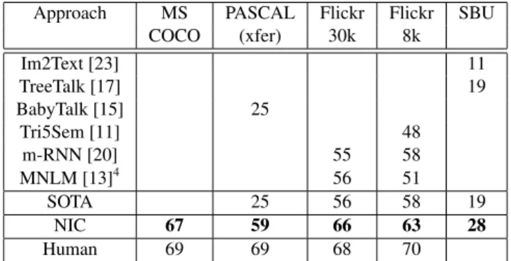
We report our main results on all the relevant datasets in Ta-ble 1. Since PASCAL does not have a training set, we used the system trained using MSCOCO (arguably the largest and highest quality dataset for this task). The state-of-the-art results for PASCAL and SBU did not use image fea-tures based on deep learning, so arguably a big improve-ment on those scores comes from that change alone. The Flickr datasets have been used recently [11, 20, 13], but mostly evaluated in a retrieval framework. A notable ex-ception is [20], where they did both retrieval and genera-tion, and which yields the best performance on the Flickr datasets up to now.
Human scores in Table 1 were computed by comparing one of the human captions against the other four. We do this for each of the five raters, and average their BLEU scores. Since this gives a slight advantage to our system, given the BLEU score is computed against five reference sentences and not four, we add back to the human scores the average difference of having five references instead of four.
Given that the field has seen some impressive advances in the last years, we do think it is more meaningful to report BLEU at a bigram or trigram level. Our results on Flickr8k are reported in Table 2 and show significant improvement with respect to [20] (similar trends are observed for BLEU at higher levels on Flickr30k).
Approach MS PASCAL Flickr Flickr SBU COCO (xfer) 30k 8k Im2Text [23] 11 TreeTalk [17] 19 BabyTalk [15] 25 Tri5Sem [11] 48 m-RNN [20] 55 58 MNLM [13]4 56 51 SOTA 25 56 58 19 NIC 67 59 66 63 28 Human 69 69 68 70
Table 1. BLEU-1 scores. We only report previous work results when available. SOTA stands for the current state-of-the-art.
Approach BLEU-1 BLEU-2 BLEU-3
m-RNN [20] 58 28 23
NIC-8k 63 41 27
NIC-30k 67 45 30
Table 2. BLEU-{1,2,3}scores, on Flickr8k. NIC-30k is our model trained on Flickr30k, while NIC-8k is trained on Flickr8k.
4.3.3 Transfer Learning, Data Size and Label Quality
Since we have trained many models and we have several testing sets, we wanted to understand whether we could transfer a model to a different dataset, and how much the mismatch in domain would be compensated with e.g. higher quality labels or more training data.
The most obvious case for transfer learning is between Flickr30k and Flickr8k. The two datasets are similarly la-beled as they were created by the same group. Indeed, when training on Flickr30k (with about 4 times more training data), the results obtained are significantly better, as seen in Table 2. It is clear that in this case, we see gains by adding more training data since the whole process is data-driven and overfitting prone. MSCOCO is even bigger (5 times more training data than Flickr30k), but since the col-lection process was done differently, there are likely more differences in vocabulary and a clearer mismatch. Indeed, all the BLEU scores degrade by 10 points (e.g. BLEU-1 is only 54). Nonetheless, the descriptions are still reasonable. Since PASCAL has no official training set and was collected independently of Flickr and MSCOCO, we re-port transfer learning from MSCOCO (in Table 1). Doing transfer learning from Flickr30k yielded worse results with BLEU-1 at 53 (cf. 59).
Lastly, even though SBU has weak labeling (i.e., the la-bels were captions and not human generated descriptions), the task is much harder with a much larger and noisier vo-cabulary. However, much more data is available for train-ing. When running the MSCOCO model on SBU, our per-formance degrades from 28 down to 16.
4We computed these BLEU scores with the outputs that the authors of
4.3.4 Generation Diversity Discussion
Having trained a generative model that givesp(S|I), an ob-vious question is whether the model generates novel cap-tions, and whether the generated captions are both diverse and high quality.
Table 3 shows some samples when returning the N-best list from our beam search decoder instead of the best hy-pothesis. Notice how the samples are diverse and may show different aspects from the same image. The agreement in BLEU score between the top 15 generated sentences is 58, which is similar to that of humans among them. This indi-cates the amount of diversity our model generates. In bold are the sentences that are not present in the training set. If we take the best candidate, the sentence is present in the training set 80% of the times. This is not too surprising given that the amount of training data is quite small, so it is relatively easy for the model to pick “exemplar” sentences and use them to generate descriptions. If we instead analyze the top 15 generated sentences, about half of the times we see a completely novel description, but still with a similar BLEU score, indicating that they are of enough quality, yet they provide a healthy diversity.
A man throwing a frisbee in a park.
A man holding a frisbee in his hand. A man standing in the grass with a frisbee.
A close up of a sandwich on a plate.
A close up of a plate of food with french fries. A white plate topped with a cut in half sandwich. A display case filled with lots of donuts.
A display case filled with lots of cakes.
A bakery display case filled with lots of donuts.
Table 3. N-best examples from the MSCOCO test set. Bold lines indicate a novel sentence not present in the training set.
4.3.5 Ranking Results
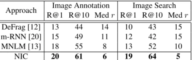
While we think ranking is an unsatisfactory way to evalu-ate description generation from images, many papers report ranking scores, using the set of testing captions as candi-dates to rank given a test image. The approach that works best on these metrics (MNLM), specifically implemented a ranking-aware loss. Nevertheless, NIC is doing surprisingly well on both ranking tasks (ranking descriptions given im-ages, and ranking images given descriptions), as can be seen in Tables 4 and 5. Note that for the Image Annotation task, we normalized our scores similar to what [20] used.
4.3.6 Human Evaluation
Figure 4 shows the result of the human evaluations of the descriptions provided by NIC, as well as a reference system
Approach Image Annotation Image Search R@1 R@10 Medr R@1 R@10 Medr
DeFrag [12] 13 44 14 10 43 15 m-RNN [20] 15 49 11 12 42 15
MNLM [13] 18 55 8 13 52 10
NIC 20 61 6 19 64 5
Table 4. Recall@k and median rank on Flickr8k.
Approach Image Annotation Image Search R@1 R@10 Medr R@1 R@10 Medr
DeFrag [12] 16 55 8 10 45 13 m-RNN [20] 18 51 10 13 42 16
MNLM [13] 23 63 5 17 57 8
NIC 17 56 7 17 57 7
Table 5. Recall@k and median rank on Flickr30k.
Figure 4. Flickr-8k: NIC: predictions produced by NIC on the Flickr8k test set (average score: 2.37); Pascal: NIC: (average score: 2.45);COCO-1k: NIC: A subset of 1000 images from the MSCOCO test set with descriptions produced by NIC (average score: 2.72);Flickr-8k: ref: these are results from [11] on Flickr8k rated using the same protocol, as a baseline (average score: 2.08);
Flickr-8k: GT: we rated the groundtruth labels from Flickr8k us-ing the same protocol. This provides us with a “calibration” of the scores (average score: 3.89)
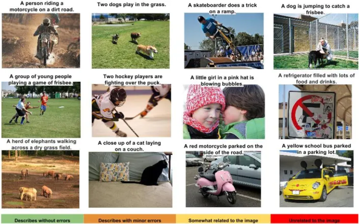
and groundtruth on various datasets. We can see that NIC is better than the reference system, but clearly worse than the groundtruth, as expected. This shows that BLEU is not a perfect metric, as it does not capture well the difference between NIC and human descriptions assessed by raters. Examples of rated images can be seen in Figure 5. It is interesting to see, for instance in the second image of the first column, how the model was able to notice the frisbee given its size.
Figure 5. A selection of evaluation results, grouped by human rating.
4.3.7 Analysis of Embeddings
In order to represent the previous word St−1 as input to the decoding LSTM producingSt, we use word embedding
vectors [21], which have the advantage of being indepen-dent of the size of the dictionary (contrary to a simpler one-hot-encoding approach). Furthermore, these word embed-dings can be jointly trained with the rest of the model. It is remarkable to see how the learned representations have captured some semantic from the statistics of the language. Table 4.3.7 shows, for a few example words, the nearest other words found in the learned embedding space.
Note how some of the relationships learned by the model will help the vision component. Indeed, having “horse”, “pony”, and “donkey” close to each other will encourage the CNN to extract features that are relevant to horse-looking animals. We hypothesize that, in the extreme case where we see very few examples of a class (e.g., “unicorn”), its proximity to other word embeddings (e.g., “horse”) should provide a lot more information that would be completely lost with more traditional bag-of-words based approaches.
5. Conclusion
We have presented NIC, an end-to-end neural network system that can automatically view an image and generate
Word Neighbors
car van, cab, suv, vehicule, jeep boy toddler, gentleman, daughter, son street road, streets, highway, freeway horse pony, donkey, pig, goat, mule computer computers, pc, crt, chip, compute Table 6. Nearest neighbors of a few example words
a reasonable description in plain English. NIC is based on a convolution neural network that encodes an image into a compact representation, followed by a recurrent neural net-work that generates a corresponding sentence. The model is trained to maximize the likelihood of the sentence given the image. Experiments on several datasets, including Pascal, Flickr8k, Flickr30k and SBU, show the robustness of NIC in terms of qualitative results (the generated sentences are very reasonable) and quantitative evaluations, using either ranking metrics or BLEU, a metric used in machine trans-lation to evaluate the quality of generated sentences. It is clear from these experiments that, as the size of the avail-able datasets for image description increases, so will the performance of approaches like NIC. Furthermore, it will be interesting to see how one can use unsupervised data, both from images alone and text alone, to improve image
description approaches.
Acknowledgement
We would like to thank Geoffrey Hinton, Ilya Sutskever, Quoc Le, Vincent Vanhoucke, and Jeff Dean for useful dis-cussions on the ideas behind the paper, and the write up.
References
[1] A. Aker and R. Gaizauskas. Generating image descriptions using dependency relational patterns. InACL, 2010. [2] D. Bahdanau, K. Cho, and Y. Bengio. Neural
ma-chine translation by jointly learning to align and translate.
arXiv:1409.0473, 2014.
[3] K. Cho, B. van Merrienboer, C. Gulcehre, F. Bougares, H. Schwenk, and Y. Bengio. Learning phrase representations using RNN encoder-decoder for statistical machine transla-tion. InEMNLP, 2014.
[4] J. Donahue, Y. Jia, O. Vinyals, J. Hoffman, N. Zhang, E. Tzeng, and T. Darrell. Decaf: A deep convolutional acti-vation feature for generic visual recognition. InICML, 2014. [5] D. Elliott and F. Keller. Image description using visual
de-pendency representations. InEMNLP, 2013.
[6] A. Farhadi, M. Hejrati, M. A. Sadeghi, P. Young, C. Rashtchian, J. Hockenmaier, and D. Forsyth. Every pic-ture tells a story: Generating sentences from images. In
ECCV, 2010.
[7] R. Gerber and H.-H. Nagel. Knowledge representation for the generation of quantified natural language descriptions of vehicle traffic in image sequences. InICIP. IEEE, 1996. [8] Y. Gong, L. Wang, M. Hodosh, J. Hockenmaier, and
S. Lazebnik. Improving image-sentence embeddings using large weakly annotated photo collections. InECCV, 2014. [9] A. Graves. Generating sequences with recurrent neural
net-works.arXiv:1308.0850, 2013.
[10] S. Hochreiter and J. Schmidhuber. Long short-term memory.
Neural Computation, 9(8), 1997.
[11] M. Hodosh, P. Young, and J. Hockenmaier. Framing image description as a ranking task: Data, models and evaluation metrics.JAIR, 47, 2013.
[12] A. Karpathy, A. Joulin, and L. Fei-Fei. Deep fragment em-beddings for bidirectional image sentence mapping. NIPS, 2014.
[13] R. Kiros, R. Salakhutdinov, and R. S. Zemel. Unifying visual-semantic embeddings with multimodal neural lan-guage models. InarXiv:1411.2539, 2014.
[14] R. Kiros and R. Z. R. Salakhutdinov. Multimodal neural lan-guage models. InNIPS Deep Learning Workshop, 2013. [15] G. Kulkarni, V. Premraj, S. Dhar, S. Li, Y. Choi, A. C. Berg,
and T. L. Berg. Baby talk: Understanding and generating simple image descriptions. InCVPR, 2011.
[16] P. Kuznetsova, V. Ordonez, A. C. Berg, T. L. Berg, and Y. Choi. Collective generation of natural image descriptions. InACL, 2012.
[17] P. Kuznetsova, V. Ordonez, T. Berg, and Y. Choi. Treetalk: Composition and compression of trees for image descrip-tions.ACL, 2(10), 2014.
[18] S. Li, G. Kulkarni, T. L. Berg, A. C. Berg, and Y. Choi. Com-posing simple image descriptions using web-scale n-grams. InConference on Computational Natural Language Learn-ing, 2011.
[19] T.-Y. Lin, M. Maire, S. Belongie, J. Hays, P. Perona, D. Ra-manan, P. Doll´ar, and C. L. Zitnick. Microsoft coco: Com-mon objects in context.arXiv:1405.0312, 2014.
[20] J. Mao, W. Xu, Y. Yang, J. Wang, and A. Yuille. Ex-plain images with multimodal recurrent neural networks. In
arXiv:1410.1090, 2014.
[21] T. Mikolov, K. Chen, G. Corrado, and J. Dean. Efficient estimation of word representations in vector space. InICLR, 2013.
[22] M. Mitchell, X. Han, J. Dodge, A. Mensch, A. Goyal, A. C. Berg, K. Yamaguchi, T. L. Berg, K. Stratos, and H. D. III. Midge: Generating image descriptions from computer vision detections. InEACL, 2012.
[23] V. Ordonez, G. Kulkarni, and T. L. Berg. Im2text: Describ-ing images usDescrib-ing 1 million captioned photographs. InNIPS, 2011.
[24] K. Papineni, S. Roukos, T. Ward, and W. J. Zhu. BLEU: A method for automatic evaluation of machine translation. In
ACL, 2002.
[25] C. Rashtchian, P. Young, M. Hodosh, and J. Hockenmaier. Collecting image annotations using amazon’s mechanical turk. In NAACL HLT Workshop on Creating Speech and Language Data with Amazon’s Mechanical Turk, pages 139– 147, 2010.
[26] O. Russakovsky, J. Deng, H. Su, J. Krause, S. Satheesh, S. Ma, Z. Huang, A. Karpathy, A. Khosla, M. Bernstein, A. C. Berg, and L. Fei-Fei. ImageNet Large Scale Visual Recognition Challenge, 2014.
[27] P. Sermanet, D. Eigen, X. Zhang, M. Mathieu, R. Fergus, and Y. LeCun. Overfeat: Integrated recognition, localization and detection using convolutional networks. arXiv preprint arXiv:1312.6229, 2013.
[28] R. Socher, A. Karpathy, Q. V. Le, C. Manning, and A. Y. Ng. Grounded compositional semantics for finding and describ-ing images with sentences. InACL, 2014.
[29] I. Sutskever, O. Vinyals, and Q. V. Le. Sequence to sequence learning with neural networks. InNIPS, 2014.
[30] C. Szegedy, W. Liu, Y. Jia, P. Sermanet, S. Reed, D. Anguelov, D. Erhan, V. Vanhoucke, and A. Rabinovich. Going deeper with convolutions. InarXiv:1409.4842, 2014. [31] B. Z. Yao, X. Yang, L. Lin, M. W. Lee, and S.-C. Zhu. I2t: Image parsing to text description. Proceedings of the IEEE, 98(8), 2010.
[32] P. Young, A. Lai, M. Hodosh, and J. Hockenmaier. From im-age descriptions to visual denotations: New similarity met-rics for semantic inference over event descriptions. InACL, 2014.
[33] W. Zaremba, I. Sutskever, and O. Vinyals. Recurrent neural network regularization. InarXiv:1409.2329, 2014.
![Figure 3. LSTM model combined with a CNN image embedder (as defined in [30]) and word embeddings](https://thumb-us.123doks.com/thumbv2/123dok_us/1841254.2766968/4.918.116.387.106.321/figure-lstm-model-combined-image-embedder-defined-embeddings.webp)