GRIPS Discussion Paper 15-02
A Fiscal Perspective on the Sustainability
of Japanese Government Debt
Tatsuya Takeda
April 2015
National Graduate Institute for Policy Studies 7-22-1 Roppongi, Minato-ku,
A Fiscal Perspective on the Sustainability
of Japanese Government Debt
Tatsuya TAKEDA
∗National Graduate Research Institute for Policy Studies (GRIPS)
April 16, 2015
Abstract
Japan’s outstanding debt keeps increasing and there are concerns regarding its sustainability. Nevertheless, the financial market seems to be neglecting such concern. Its growing debt level and subdued general price level are not easy to explain from the fiscal theory of price level (FTPL) either. Thus, Japan has been a “puzzle” for many. This puzzle can be better understood with extended definition of government and its debt. If Fiscal Investment and Loan Program (FILP) agencies are included in the definition of “government”, Japan was running surpluses for several years since 2000, implied by the change in the real value of the government’s total debt including loans owed to the private sector. This paper introduces the new measurement scheme for the fiscal state of Japan and its implication on FTPL calculations to analyze the puzzle and to address the debt sustainability issue of Japan through FTPL perspectives on “Abenomics”.
I
Introduction
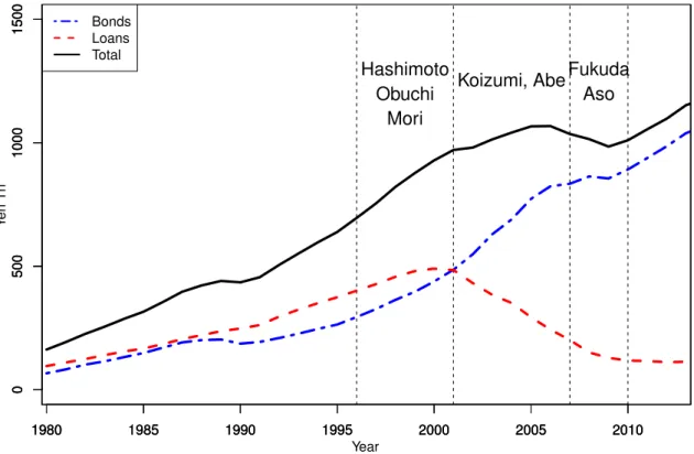
Japan’s fiscal position has been a concern for many policy makers and economists around the world. As Hoshi and Ito (2012, p.3) summarizes, “[m]any academic papers written in the last decade have concluded that the current Japanese government deficits and debts are not sustainable.” In terms of market value, 911 trillion yen of Japanese Government Bonds (JGBs), 157 trillion yen Treasury Discount Bills (TBs), and 163 trillion yen of loans are outstanding as of March, 2014. Of the loans, 56 trillion yen is borrowed by the central government and 107 trillion yen is borrowed by Fiscal Investment and Loan Program (FILP) agencies. Figure I-1 shows how this large amount of debt has grown over the past 25 years. JGB is mostly held by domestic investors1 and this fact is typically
quoted as a reason for JGB market’s stability. However, as Hoshi and Ito (2012, p.14) discusses, “Japanese government debt will soon exceed private sector financial assets” possibly within 10 years. Still the JGB market is quite calm and nominal interest rates are extremely low.
1980 1985 1990 1995 2000 2005 2010 0 500 1000 1500 Hashimoto Obuchi Mori
Koizumi, AbeFukuda Aso 1980 1985 1990 1995 2000 2005 2010 0 500 1000 1500 1980 1985 1990 1995 2000 2005 2010 0 500 1000 1500 Year Y en Tn Bonds Loans Total
Figure I-1. History of Japanese debt (market value): A casual observation of bonds leads to an impression of fast growing debt but the total debt level has not materially changed sine 2001 during the era of Koizumi, Abe, Fukuda, and Aso if loans are included.
In the context of the fiscal theory of price level (FTPL), an increase in the nominal value of the
government debt should be accompanied by either one or the combination of an increase in the general price level and an increase in the present value of future government surpluses. The price level did not rise and the government surplus as casually observed in the primary balance was generally negative (or deficit) over the past 25 years except for a very brief period around 1990.
The surprisingly stable JGB market and the subdued price level despite the growing debt level and the continuing primary balance deficit are the two sides of the same puzzle. The government debt price should fall when there is too much of them in the market and there is no clear sign of future decrease in volume through budget surpluses. The general price level should rise when the nominal value of the government debt increases without corresponding increase in the present value of future surpluses. Both theories imply an economy with higher price level with lower real values for the government debts.
This puzzle has made it difficult for economists and policy makers to understand the true nature of the issue of debt sustainability in Japan. The stable JGB market has led some to believe that the Japanese economy is different from the US or European economies because there is sufficient domestic savings to support the government deficits.2 The subdued price level has led others to
conclude that the fiscal theory is not quite applicable to Japan; rather, the monetary policy dominates the fiscal policy and thus the open market monetary operation by the Bank of Japan (BoJ) is effective in controlling inflation. If indeed there is not sufficient domestic savings to support the growing government debts as Hoshi and Ito (2012) suggests and the fiscal constraint is binding, the JGB market may be at the brink of sell-offand BoJ may not be able to control a fiscal inflation at the end of the current aggressive monetary easing, in which people try to dispose of all government liabilities including both money and JGBs, making it difficult for BoJ to contract the economy as it will not be able to conduct open market operations.3
This paper attempts to provide a new measurement of the government debt and the derived sur-pluses to bridge the gap between the theory and the data. A casual observation of JGBs leads to an impression that the Japanese government debt burden has kept increasing for 25 years and accelerated from 2001. However, the government borrows funds from the private sector not only in the form of
2Sims (2013) makes an interesting observation on the US and European economies with respect to their common difficulty in assuring effective partnership between fiscal and monetary authorities. He claims “it is not hard to imagine Congress blaming the Fed for the painful decisions it faces and in the process casting doubt on its commitment to recap-italize the Fed” for the US and “if the capital called for were substantial, and the call came in the wake of ECB policy actions that were politically unpopular in some countries, the provision of capital might not be automatic” for Europe. (Sims, 2013, p.567)
3Sims (2013) also mentions the risk of people realizing that a central bank not having sufficient assets to sell in order to contract the economy if its balance sheet is impaired and the fiscal authority is not willing to support.
bonds and bills but also in the form of loans, most of which has been used to finance the FILP finan-cial agencies. If such loans are included in the definition of the government debt, one can see that the market value of debt did not increase during the first several years of 2000s and it only started to increase again after the global financial crisis in 2008. Figure I-1 suggests that fiscal consolidation in Japan led by Prime Ministers Koizumi and Abe was successful in stabilizing Japan’s fiscal condition. The trend continued on throughout the Liberal Democratic Party (LDP) rule until 2009 under Prime Ministers Fukuda and Aso. The Japanese government debt started to grow again when the Democratic Party of Japan (DPJ) came into power in 2009 right after the global financial crisis, even before the 2011 earthquake.
This paper suggests that fiscal dominance exists in Japan if one properly accounts for the FILP financial agencies as a part of the government and the implied surplus is used as a measure of surplus in the government sector. The existence of fiscal dominance indicates a possibility of fiscal inflation in Japan beyond the control of BoJ.
II
Literature
II. 1 On Japanese debt sustainability
Japan has a large amount of debt outstanding by any measurement. Economists have tried to reconcile the growth of JGBs in the past 25 years since the burst of bubble, particularly in the past 15 years since the turn of the century, and Japan’s deflationary experience and the stable JGB market during the same period.
The sustainability of Japanese government debt situation has been extensively discussed among economists and various reports have been published by international organizations such as IMF as well. IMF (2011) suggests the slow growth and policy missteps as the root cause of the Japanese fiscal imbalances and also mentions that “market sentiment toward sovereigns with unsustainably large fiscal imbalances can shift abruptly, with adverse effects on debt dynamics.” It also refers to the high corporate savings and declining household savings due to demographic change and stagnating wages. Although the private saving remains high, the composition has changed. Hoshi and Ito (2012) claims that the private saving supporting the government fiscal imbalances has a ceiling and summarizes literature in this field all pointing at the dire situation of the Japanese government debt position. Doi, Ihori, and Mitsui (2006) discusses the sustainability of the Japanese government debt situation by
focusing on the JGB market and suggests that “[t]he fiscal authority has an incentive to default when the amount of debt outstanding is more than a certain level.” It also touches on the “non-Keynesian effects”, where several countries have experienced growth in private demand under tight fiscal policy. Additionally, credit rating agencies such as and Standard and Poor’s and Moody’s have continu-ously downgraded the Japanese sovereign rating. Standard and Poor’s lowered the sovereign rating of Japan to AA- in January 2011 claiming that the Japanese government would not achieve a primary balance before 2020 unless a significant fiscal consolidation program is implemented (S&P, 2011). Standard and Poor’s changed the credit outlook of Japan from stable to negative in April 2011 re-flecting the increased fiscal difficulty incurred by the Great Tohoku Earthquake in March 2011. More recently, Moody’s downgraded the Government of Japan’s debt rating from Aa3 to A1 with a stable outlook in December 2014 (Moody’s, 2014). The agency cites as the reason both the increased un-certainty of achieving debt reduction goals and the unun-certainty over the effectiveness of the growth strategy, which is the “Third Arrow” of Abenomics.
II. 2 On Fiscal Investment and Loan Program (FILP)
Information on FILP can be obtained in the official FILP report published by the Japan Ministry of Finance. Doi and Hoshi (2002) examines the financial health of the FILP agencies by studying the financial conditions of FILP recepients and concludes that “many are de facto insolvent” (Doi & Hoshi, 2002, p.1). Iwamoto (2002) states, following Doi and Hoshi (2002), “[t]he already created loss is unavoidable. What is important for the current decision making is how not to produce a further welfare loss in the future FILP programs.”
Tomita (2000) summarizes the need and the purpose of FILP reform. He states that FILP was a policy tool to mitigate failures of financial markets in its inability to provide long term risk money but a new concern has emerged about the “political failures” that FILP may have not kept up with the socio-economic changes and that it may “have placed a burden on future generations”. Iwamoto (2002) similarly concludes that FILP needs to be changed to fit “the well-developed market economy”. Watarase (2007) studies FILP from the perspective of the flow of funds and concludes that the “private to public” flow has not changed despite the FILP reform because private financial institutions still make a large amount of JGB investments. He also points out that Postal Savings, Postal Insurance, and Public Pensions were forced to purchase JGBs between 2001 and 2007 as a means of smoothing the transition of financing mechanism for FILP agencies from loans to JGBs.
II. 3 On the fiscal theory of price level (FTPL)
FTPL has been developed since 1991 by Leeper (1991), Sims (1994), Cochrane (1999, 2001, 2005), and Woodford (1999) among others. Most literature uses one period debts and is with or without money. Cochrane (1999, 2001) extends the model to use long term debts and shows FTPL is consistent with the history of surpluses and debts of the United States.
Cochrane (2001) also explores the impact of term structure on the price level evolution against exogenous shock to surpluses. He shows that any surprise shock to the government surplus can be absorbed by the nominal value change of the government debt portfolio when it contains long term debts. Since any shock to the surplus would affect the general price level immediately in a one-period debt model, this is a significant extension of the framework.
Additionally, Cochrane shows the maturity structure of long term debts affect the timing of changes in the price level in response to shocks to the surplus and suggests an optimal term struc-ture for countries hoping to control variances of price levels or inflation. In the Japanese context, a longer term structure of government bonds dampens the impact of future surplus changes on the cur-rent price levels. Japan Ministry of Finance (MoF) has been extending the average duration of JGBs both to take advantage of the low interest rate environment and to minimize refunding risks while BoJ is buying longer term JGBs, effectively shortening the government debt portfolio duration.
The policy discussion in Japan has revolved around the monetary side and there have not been many studies from the fiscal perspective. Doi (2000) follows Cochrane (1999) and Woodford (1999) and concludes that, based on data from 1955 to 1997, the monetary policy in Japan was passive during this period, the fiscal policy was active, and FTPL cannot be neglected in order to explain price levels in Japan (Doi, 2000). However, there has not been much research since then.
While being pioneering, Doi’s analysis has some room for improvement in order to be applied to the current environment. For example, Doi focuses on the central government and uses the govern-ment bonds as the proxy for the governgovern-ment obligation but Japanese governgovern-ment used to borrow a large amount in the form of loans until 2000 in FILP as discussed earlier. Another area is the nomi-nal yield of the government debts. Doi (2000) uses the average issuing yield of JGBs but it is more appropriate to use the average yield of all outstanding bonds. Finally, he uses the primary balance as the surplus instead of the implied surplus derived by the change in the privately held government debt values. This is not much of an issue for his sample period from 1955 to 1997 and for the limited scope of the central government but, as I shall show shortly, the primary balance is not a good proxy
for the overall government surplus in Japan.
This paper extends the current discussion on Japanese debt sustainability by re-scoping the gov-ernment debt and by adding a fiscal theory perspective. Further it extends existing FTPL literature on Japan in two ways. First, it uses the surplus implied by the change in the privately held government debt, which enables the analysis to cover the broadly defined government including FILP agencies. Second, it uses both bonds and loans as the government debt and the weighted average yield of out-standing debt as the nominal yield on the government debt portfolio. These two extensions provide a better vantage point to analyze and solve the Japan puzzle for FTPL.
III
Review of The Fiscal Theory of Price Level (FTPL)
There are two approaches for the determination of price level, monetary and fiscal, expressed by the following two equations as extensively used by Cochrane (2005, 2011b).4
MtVt = Ptyt (1) Bt +Mt Pt =Et Z ∞ τ=0 Λt+τ Λt st+τdτ (2)
Mt is the monetary base,Vt is the ‘velocity’ including the money multiplier, Pt is the general price
level,ytis the output,Btis the nominal value of the government debt portfolio,Λt+τ/Λtis the
stochas-tic discount factor fromttot+τ, and st+τis the real primary government surplus including seignorage
at t +τ. (1) represents the quantity theory of money (the monetary equation) and (2) is the fiscal equation.
If one assumes a stable velocity Vt = V, the monetary equation (1) determines the general price
level Pt from the policy variable Mt once the output yt is set. Then the government, or the fiscal
authority, has to adopt the surplus path st+τ which satisfies the fiscal equation (2) for given Bt and Mt. In this case, the monetary framework dominates the fiscal framework and it is called monetary
dominance, also known as the Ricardian regime. In the Ricardian policy regime, the fiscal authority chooses the level of st+τ in order to make (2) balanced for any price level Pt which is set by the
monetary authority through (1). In this framework, (1) sets the price levels and (2) follows them by choosing appropriate future surpluses. Thus, the price level is set by the quantity theory.
4Most description of the fiscal theory framework is taken from Cochrane (1999, 2001, 2005, 2011b) and Woodford (1999).
On the other hand, if the fiscal authority sets the future surplus path st+τindependently from the
output level or simply assuming it is exogenously given, the fiscal equation (2) determines the price level Pt for given Bt and Mt. In this case, the fiscal equation dominates and the monetary authority
must choose Mt that satisfies the monetary equation (1). This is the fiscal dominance, also known
as the non-Ricardian regime. Of course, there is a possibility of perfect coordination between the monetary and fiscal authorities to solve those two equations simultaneously. In the non-Ricardian policy regime, (2) does not hold for all price levels but there may be a unique Pt which makes (2)
balanced for any exogenously given sequence of st+τ. That is, the price level is set by (2), then (1)
follows this by adjusting Mt. This is the fiscal theory of price level.
Three points are worth noting regarding the relevance and the advantages of FTPL in today’s economic analyses. First, it is interesting to note that the fiscal theory of price level is completely immune to financial innovations as Cochrane (2005) emphasizes, whereas the quantity theory has difficulty explaining the economy as a larger portion of money becomes inside and as private moneys increase their significance. Financial innovations can materially affect the velocity and the demand for monetary base.
Secondly, Sims (2013, p.563) points out that “monetary and fiscal policy are tied together” now that reserve deposits at a central bank bears interests in many countries including the US and Japan. Very low interest rate level has made the short term government securities and the monetary base highly interchangeable and now even the medium term government bonds and the interest-bearing reserves have become close substitutes. He further claims that fiat money can become valueless without fiscal backing. He then concludes,
The kinds of models that have been the staple of undergraduate macroeconomics teach-ing, with price level determined by balance between “money supply” and “money de-mand”, and money supply using the “money multiplier”, are obsolete and provide little insight into the policy issues facing fiscal and monetary authorities in the last few years. (Sims, 2013, p.582)
Thirdly, as Cochrane shows, the maturity structure of debts matters in price determination for today. In general, the longer the average duration of the nominal debts is, the smaller the price variation can be today (Cochrane, 2001) and Woodford (1999) agrees. This is because the general price level is determined by the ratio of the nominal value of the government debt to the future surpluses and a longer duration debt portfolio has higher capability to adjust its nominal value.
Cochrane (2011b, p.7) expands (2) with respect toBt as follows: Bt = Z ∞ j=0 Q(tj)B (j) t dj= Z ∞ j=0 Et Λt+jPt ΛtPt+j ! B(tj)dj, (3)
whereB(tj) denotes the nominal notional amount of jyear debt at timetandQ (j)
t denotes its nominal
market value at timet. Combining (2) and (3), one obtains
Mt Pt +Z ∞ j=0 Et Λt+j ΛtPt+j ! B(tj)dj= Et Z ∞ τ=0 Λt+τ Λt st+τdτ. (4)
Therefore, “[b]y buying and selling debt at date tand later, after Etst+τ is revealed, the government
can achieve any sequence of Et
1/Pt+j
, consistent with this equation, without making any changes in surpluses. The more long-term debt outstanding – the greater B(tj) relative to B(0)t – the better the trade off” (Cochrane, 2011b, p.7).
For a country like Japan with so much government debt outstanding either compared to the GDP or to the monetary base, both the fiscal equation and the quantity theory are important.
IV
Definition of surplus, debts, and the government
In order to shed some light on the fiscal analysis of Japan, it is beneficial to revisit the definitions of surpluses and debts and the scope of the government of Japan. This paper uses implied (or economic) surpluses derived from the change in debt values following Cochrane including both bonds and loans. It also considers FILP agencies as a part of the government for the purpose of fiscal analysis.
IV. 1 Scope of the government and its debts
Most researches including Doi (2000) use the central government as the definition of government in their analyses. On the other hand, Hoshi and Ito (2012, pp.4–5) suggests the following three different definitions of government debts, which implies multiple definitions for the scope of the government as well.
1. JGB (including FILP bonds), long term borrowings, TB, and explicit government guarantees.
3. JGB (excluding FILP bonds), TB, explicit government guarantees, and liabilities in
the social security funds.
The first is used for reports to IMF while the third is used for National Income Accounting.
This research defines the government as the combination of the central government, the Bank of Japan (BoJ), and Fiscal Investment and Loan Program (FILP) agencies. FTPL treats central banks as a part of the government because it focuses on the public sector’s debts to the private sector and the monetary base is a part of what the government owes to the private sector.5 All kinds of borrowed
money such as bonds, bills, and loans are included in debts.
IV. 2 Implied (or economic) surplus
The government collects money in one way or another, mostly by tax, and spends it to provide neces-sary pubic services. The money coming in and going out must be balanced in the long run but there is a surplus or a deficit in each year. There are many ways to measure those surpluses such as the primary balance, whether they are positive or negative. I use the implied surplus following Cochrane (1999, 2011b, and others) based on an accounting identity in which the change in borrowing is equal to the surplus.6 It might be better to convert everything into real scale and still the identity holds.
Cochrane (1999) writes
st+1 = vtrt+1−vt+1, (5)
wherest+1denotes the real surplus for the period fromttot+1,vt the outstanding real value of debt7
at timet, rt+1 the real interest rate on the debt fromtto t+1. That is, vgrows fromvt tovtrt+1 with
the real interest ratert+1and the difference between this value and the actual real value of debtvt+1at
timet+1 is the surplus st+1fromttot+1. This implied (or economic) surplusst is used throughout
this paper.
5Thus, the total value of the government debt does not change when BoJ conducts monetary operations by buying or selling JGBs in the market. Please refer to Cochrane (1999, 2001, 2005, 2011b) for more detailed discussion on this point. 6For example, if a company borrows 100 in yeartat an interest rate of 10% per period and has only notional 90 debt outstanding att+1, the debt should have grown to 110 with the accrued interest but is in fact 90 and this reduction of 20 in debt must come from somewhere else, which I call the surplus. What if the market value of the debt comes down from yearttot+1? It still means there is less to be returned to the creditors and I consider it as a surplus generated by a proper debt management, or by a pure luck.
IV. 3 Treatment of FILP in this paper
This paper includes FILP in the scope of the government for three reasons. First of all, FILP is too big to be ignored. As Doi and Hoshi (2002) says, most countries have government sponsored investment and loan programs but the amount of funds that go through FILP is comparable to the central government as Figure IV-1 shows. Further, FILP agencies’ investments are made as an integral part of fiscal policies to support the creation of future tax base just like ordinary spending by the general account. As MoF (2014) says, FILP is a tool of fiscal policy and its plan is annually submitted to the Diet (the Japanese parliament) for deliberations and resolutions. FILP agencies are closely linked with various special accounts of Japanese government budget, which need to be captured in fiscal analyses. 1980 1985 1990 1995 2000 2005 2010 0 200 400 600 800 1000 1980 1985 1990 1995 2000 2005 2010 0 200 400 600 800 1000 Year Y en Tn Central Government FILP Agencies
Figure IV-1.Debt comparison between the central government and the FILP agencies: The outstanding debt value of the FILP agencies was the same or more than the debt value of the central government until the FILP reform of 2001.
One might argue that some FILP agencies make investments and not just expend the funds and therefore FILP should be treated differently from the central government. In other words, there is an argument that FILP liabilities are backed by FILP’s investments. However, FILP financial agencies are making those investments for policy reasons rather than for economic return reason and, in fact,
Doi and Hoshi (2002) claims that many of FILP agencies’ investments are insolvent and that they are supported by taxpayers. In addition, a government spends money with an intention to collect the money with interest. That is, a government cannot run perpetual deficits. If, and when, people come to believe that the government will not earn enough surpluses in the future, they realize there will be more government’s debts in the market than they need to pay the taxes in the future and they will try to get rid of them, causing a “run” on the government (Cochrane, 2011a). From this perspective, all government’s spending must be considered backed by future tax income in a stable economy. Then, there is not much difference between the central government’s activities and those of FILP agencies.
IV. 4 FILP reform in 2001
FILP was set up to provide financial support to long term infrastructure investments and other areas where private investment was not sufficient. Funds from Postal Saving, Postal Insurance, and Public Pension were deposited at the Trust Fund Bureau (TFB) of MoF, which in turn lent those funds to FILP agencies.8 The FILP agencies also borrow funds directly from the private financial institutions.
As the 2014 report on FILP by MoF describes, FILP is run as a part of the overall policy set (MoF, 2014). This is also evidenced by the most recent stimulus package announced by the Japanese gov-ernment on January 9, 2015, where the govgov-ernment announced 3.1 trillion yen of additional spending from the general account accompanied by 0.1 trillion yen increase in FILP.
The Japanese government was quite “big” because of FILP agencies and their associated special account budgets. Further, FILP has become obsolete as Iwamoto (2002) says “[a] system that worked very well in a postwar reconstruction period stumbled in recent times. The system has to be changed so that it fits the well-developed market economy.”
The Liberal Democratic Party (LDP) recovered the premiership back from the coalition of “anti-LDP” parties in 1996. The FILP reform discussion was started and Outline for Fundamental Reform of the Fiscal Investment and Loan Program was published in November 19979and a detailed blueprint was announced in August 1999.10 Legislation to abolish the Trust Fund Bureau was passed in May
2000 to be effective from April 2001.11 At the same time, the direct flow of fund from the public
8Postal Insurance also made direct loans to FILP agencies. Doi and Hoshi (2002, p.39) has a detailed visual description of the flow of funds.
9Please see www.mof.go.jp/english/about mof/councils/fund operation/e1a028.htm 10“Zaisei toyushi no bapponteki kaikaku ni kakaru giron no seiri” in
https://www.mof.go.jp/about mof/councils/unyosin/report/1a1503.htm
11For the more graphical but official description of the FILP reform in English, please see www.mof.go.jp/english/filp/filp report/zaito2011/pdf/p07-1.pdf
1980 1985 1990 1995 2000 2005 2010 2015 0 100 200 300 400 500 1980 1985 1990 1995 2000 2005 2010 2015 0 100 200 300 400 500 1980 1985 1990 1995 2000 2005 2010 2015 0 100 200 300 400 500 Year Y en Tn Bonds Loans Total
Figure IV-2.Evolution of funding for FILP financial agencies: FILP agencies used to fund almost entirely by loans through Trust Fund Bureau and direct loans from Postal Insurance but shifted their main funding channel to FILP bonds since 2000.
pension to FILP was stopped by the legislation in 1999.
Mr. Koizumi became the prime minister in April 2001 and carried through the reform. His main focus was to privatize Postal Saving and Postal Insurance so that they invest their customers’ funds just like other financial service providers. The abolishment of TFB was meant to require FILP agencies to secure their own fundings but this part of reform was not fully executed as the FILP agencies now finance themselves mostly by issuing FILP bonds under full guarantee of the government, which are perfectly fungible with regular JGBs. Therefore, the amount of JGB issuance grew substantially from 2001 to compensate for the decline of the loan channel.12 Figure IV-2 shows how this switch
from loans to bonds took place and the total funding decreased. Postal Saving and Postal Insurance, together with Public Pension, are significant investors of JGBs. Thus, the funds are still flowing from Postal Saving, Postal Insurance, and Public Pension to FILP agencies but now in the form of bonds rather than loans. That is, the flow of funds from the private sector to FILP agencies was only transformed from loans to bonds and, thus, the total amount of fund flowing to FILP has not declined
12There is a little amount of bonds issued by FILP agencies with their own credit but the majority of the funding is done through FILP bonds.
so much as the portion of fund in the form of loans has.
V
Empirical analyses
V. 1 Data and variables
The analysis period of this paper is from 1981 to 2014 and three sources of data are used. They are Flow of Funds report from BoJ13, SNA(System of National Accounts of Japan) from Cabinet Office14, both based on 93SNA, and the websites of MoF.
V. 1 (a) Flow of Funds report
The report is compiled and published by BoJ on the market value basis wherever possible and the numbers for the Japanese fiscal year end (March) are used for all entries. For the complete listing of data series, please refer to Appendix C.
Bonds Japanese central government issues Japanese Government Bonds (JGBs) and FILP Fund issues FILP Bonds, which are completely fungible with and undistin-guishable from JGBs. Additionally, FILP agencies issue bonds with their own credit (FILP Agency Bonds). All three types of bonds’ outstanding market values are re-ported. Intra-government holdings are net out to calculate the bonds held by the private sector.
Discount Bills Japanese central government issues Treasury Discount Bills (TBs) with
up to 1 year maturity for short term financing. These securities are often purchased by various entities to temporarily park investment or operational funds. The market value is reported in Flow of Funds reports and intra-government holdings are netted out.
Loans Central government borrows money from private financial institutions and special
financial institutions such as Postal Saving, Postal Insurance, and Public Pension. FILP agencies borrow money from private financial institutions. Those amounts are reported at market value wherever possible. Bank of Japan provides loans to private financial institutions and this loan value is subtracted from the total value.
13www.stat-search.boj.or.jp/index en.html 14www.esri.cao.go.jp/en/sna/menu.html
FILP Fund Money flows through FILP Special Account. Funds from Postal Saving,
Postal Insurance and Public Pension are deposited into the fund, which is then dis-tributed to FILP agencies for public finance purpose. It is a liability account for FILP agencies but an asset for the central government. The net liability is calcu-lated by subtracting the latter from the former. The numbers are reported at the notional value, rather than the market value.
Financial Assets Market value of foreign securities held by the government for foreign exchange reserves15 and private sector securities held by BoJ are reported at the
market value.
Monetary Base Cash in circulation and reserves held at BoJ.
V. 1 (b) National Accounts of Japan
Cabinet Office of the government reports these figures on a quarterly basis. Two annual series are taken: H21 Series which covers from March 1981 to March 2010 and H24 Series which covers from March 1995. H24 Series is used where possible and H21 Series is simply rescaled in March 1995 and used for 1981 to 1994.
Deflator GDP deflator, 100 in the calendar year 2005
Consumption Annual nominal consumption for both public and private sectors
Primary Balance Reported in SNA as net government lending after adjustment for
in-terest payments
V. 1 (c) MoF websites
The weighted average outstanding nominal yields of JGBs are obtained from the MoF website.16 This weighted average is calculated only for JGBs and excludes discount securities (TBs). TB yields are obtained from another page using the 1 year point on the yield curve.17
15In Japan, foreign reserves are entirely managed and held by MoF instead of BoJ. BoJ simply executes transactions on behalf of MoF.
16www.mof.go.jp/jgbs/reference/appendix/zandaka05.htm 17www.mof.go.jp/jgbs/reference/interest rate/data/jgbcm all.csv
V. 1 (d) Variables
The following variables are constructed from the above data following Cochrane (1999).
vt: Real value of government debts held by the private sector, constructed from the Flow
of Funds report on the basis of market values. In order to derive the privately held debt value, government debt value held by the government agencies including BoJ is subtracted from the total liability value of the central government and the FILP agencies. Further, the foreign securities held by the government as a foreign reserve and the private securities held by BoJ are subtracted from the liabilities as those se-curities are financial assets usable by the government to pay down its debts. Values are converted to real numbers by the GDP deflator.
πt: Inflation πt is defined by the change of GDP deflator from time t − 1 to t. I.e.,
πt = Pt/Pt−1.
rt: Real return of government debt portfolio fromt−1 totcalculated from the weighted
average nominal yield of the government’s total debt portfolio and the inflation. In order to calculate the overall nominal portfolio yield of the government debt, this paper calculates the weighted average between TBs and JGBs assuming zero interest rate for the monetary base and further assumes that the loans have the same weighted average nominal yield as JGBs.
MoF websites’ JGB weighted average yield and 1 year JGB yield are averaged with the market value weight of JGBs and TBs. This weighted average yield is also assumed for the government loans. The monetary base is assumed to have zero interest rate and the overall weighted average nominal rate of the government debt portfolio (JGBs, TBs, loans, and monetary base) is calculated. The inflation from
t−1 tot(πt) is then subtracted from this weighted average rate to producert. sct: Surplus implied by the change in the government debt value and the interest rate, as
expressed in (5), is divided by consumption for normalization following Cochrane (1999, p.361). The division by consumption “scale[s] variables with growth, pro-ducing plausibly stationary series” while avoiding “business-cycle output variation in the surplus measure” which division by output may incur.
dct: Real growth of consumption fromt−1 tot.
Further,vctanddctare log linearized around their steady states (sample means) butsctis a simple
deviation from the sample mean as the value can be negative.
1980 1985 1990 1995 2000 2005 2010 2015 0 2 4 6 8 1980 1985 1990 1995 2000 2005 2010 2015 0 2 4 6 8 Year P er Cent Nominal Rates Real Rates
Figure V-1.Nominal and real rates: Weighted average rates of outstanding bonds, bills and monetary base kept declining throughout the analysis period. The real rate suddenly dropped around 1990 because of the bubble inflation.
Figure V-1 shows the evolution of weighted averaged rates used in the analysis for the case including loans. Nominal rates were high in the 1980s and continued to drop while real rates did not fall as much because of deflation. The sudden drop in real rates toward the end of 1980s is a result of spiking inflation.
V. 2 Implied surpluses
Figure V-2 compares the primary balance reported in SNA to the implied surplus st in (5). st,
including FILP, fluctuates more than the primary balance but the overall fit seems reasonable. The correlation between the two series is 0.78 before year 2000 and 0.91 thereafter. It is interesting to note that the implied surplus is mostly positive during the first decade of this century, which is consistent with flat or slightly decreasing trend of total debts presented in Figure I-1.
1980 1985 1990 1995 2000 2005 2010 2015 −50 0 50 1980 1985 1990 1995 2000 2005 2010 2015 −50 0 50 1980 1985 1990 1995 2000 2005 2010 2015 −50 0 50 Year Y en Tn
Primary Balance as reported Implied Surplus excluding FILP Implied Surplus including FILP
Figure V-2.Surplus comparison: Implied surplus from the change in debt values has wider variation than SNA reported Primary Balance because it is more inclusive but the innovation patterns are similar. Implied surpluses show clear surplus, rather than deficit, in the first several years in this century when FILP is included.
The implied surplus also fluctuates more than the primary balance even FILP is excluded. How-ever, it is worth noting that the implied surplus excluding FILP fluctuates around the primary balance after 2001 while the implied surplus including FILP stays above the primary balance in the same period.18
Figure V-3 summarizes the evolution of implied real surplus, real debt value, and the weighted average real interest rate of government debt portfolio. The figure looks very similar to Figure 8 in Cochrane (1999, p.364) as the surplus and the debt growth correlate negatively. Real interest rates were high in 1980s and 1990s with a sudden drop in late 1980s due to high inflation during the peak of the economic bubble. Real debt value was growing fast in 1980s and 1990s due to both high interest rates and negative surplus (deficit). Interest rates kept falling and the real debt value was stable during the first decade of this century due to lower interest rate and surplus including FILP. The Global Financial Crisis in 2008 and the Great Tohoku Earthquake in 2011 brought the Japanese government
18The correlation between the implied surpluses excluding FILP and the SNA reported primary balance is 0.82 before 2000 and 0.79 thereafter. Regardless of the inclusion of FILP, the correlations drop significantly post 2000 if loans are excluded from the analysis. It falls to 0 if loans are excluded while FILP is kept in the scope of the government.
again into deficit and the real value of government debt has shown a rapid growth since 2009. 1980 1985 1990 1995 2000 2005 2010 2015 −0.2 −0.1 0.0 0.1 0.2 Year s/v and v(t)/v(t−1)
Real Interest Rate (per cent)
0 1 2 3 4 5 6 surplus/debt value debt value growth real interet rate
Figure V-3. Surplus, debt value, and interest rate: Real value of debts was growing fast in 1980s and 1990s with high interest rates and slightly negative surplus. Debt value is more influenced by surplus with declining interest rates from 2000
The next task is to analyze the observed relationship among the surplus, the real value of the government debts, and the real return on the debts.
The fiscal framework views the identity (5) as the following.
rt+1 = st+1 vt + vt+1 vt (6)
The future surpluses determine the real value of the government debts in FTPL. Thus, (6) determines the real return of the privately held government debts with the information on the future surpluses, which in turn determines the inflation from the nominal yield so that the Fischer equation holds. This relationship suggests positive correlations betweenrt+1 and st+1/vt and betweenrt+1 andvt+1/vt
(Cochrane, 1999, p.366).
On the other hand, the monetary framework views the same identity (5) differently. In the mon-etary framework, the price level is given by (1) and this will derive the real value of the government debt vt+1 from its nominal value. Then the government adjusts the value of surplus st+1 to satisfy
the identity shown in (5). Thus, (5) is also interpreted as the derivation equation for st+1. Cochrane rewrites (5) as st+1 vt = rt+1− vt+1 vt . (7)
From the monetary perspective, this equation shows how the surplus as a fraction of debt value is determined by the difference between the real rate of return on the privately held government debts and the growth rate of such debts (Cochrane, 1999, p.364), both of which are determined outside of this equation by the price levelPt set by (1).
Regarding (7), it is expected that st+1/vt has a negative correlation with vt+1/vt. On the other
handrt+1 should have a positive correlation withvt+1/vt asvt should grow atrt+1 assuming balanced
government budget. Therefore,st+1/vt andrt+1should have a weaker negative correlation. (Cochrane,
1999, p.365)
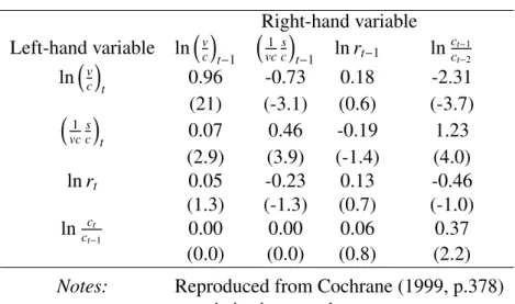
Table V-1.Correlations in Japan data
rt+1 vt+1/vt st+1/vt rt+1 1.00 0.58 -0.35 vt+1/vt 1.00 -0.97 st+1/vt 1.00
Table V-2.Correlations in US data19
rt+1 vt+1/vt st+1/vt rt+1 1.00 0.70 -0.16 vt+1/vt 1.00 -0.82 st+1/vt 1.00
Table V-2 is reproduced from Cochrane (1999, p.365). Cochrane states that the “pattern of corre-lations is what a backward-looking view with relatively stable money and hence prices might expect” and claims that it is a “puzzle” (Cochrane, 1999, p.367). Table V-1 shows my results for Japan, which have the same characteristics.20 That is, the Japanese data also seem to support a backward-looking,
or a monetary, perspective.
V. 3 VAR analysis
V. 3 (a) Explaining the correlations with a simple VAR
Cochrane solves this unintuitive correlation pattern from the FTPL perspective by showing that a very simple VAR model with an exogenous surplus process can indeed create the correlation relationships observed in Table V-1 and Table V-2 (Cochrane, 1999). Please refer to Appendix A for mathematical derivation.
19Reproduced from Cochrane (1999, p.365) 20Excluding FILP, the correlation betweenr
t+1andvt+1/vtfalls to 0.33 and betweenrt+1andst+1/vtfalls to -0.16 while betweenvt+1/vtandst+1/vtincreases to -0.99.
He starts by rewriting the accounting identity in (5) as: vt ct = 1 rt+1 ct+1 ct st+1 ct+1 + vt+1 ct+1 ! .
Further,with the following definition
β≡ E
"
ct+1 ctrt+1
#
and the log linearized21variables, he writes
vct = Et ∞ X j=1 βj sct+j. (8)
The surplus is modeled as the sum of a long term trend componentzt and a cyclical componentat
as the following.
sct = zt+at (9)
zt = ηzzt−1+εzt at = ηaat−1+εat
That is, both the long term trend and the cyclical components are modeled as AR(1) and there is no other shock element in the surplus. Cochrane views the long term trend as driven by policies such as tax and spending. Note thatηzis expected to be close to 1, i.e.,zt should be a persistent process.
Form a simple VAR, represented as
sct vct = A sct−1 vct−1 +δt. (10) 21As discussed in V. 1 (d),vc
I obtain point estimations as22 d sct vct = 0.501∗∗∗ 0.018 −0.558∗∗∗ 0.990∗∗∗ sct−1 vct−1 (11)
and, using the sample mean,
ˆ
β= 0.9896.
Just as equation (37) in Cochrane (1999, p.369), one can observe positive effect ofvct−1on sct in
(11). However, Table B-3 shows that this positive effect cannot be observed in the data excluding FILP. Further, again as Cochrane (1999) points out, both sct and vct are persistent and the negative
effect ofsct−1onvct indicates that high surplus forecasts future lower surpluses.
As Cochrane (1999) mentions, there is a structural restriction that (2, 1) element of A,a21, must be negative of (1, 1) element,a11, which is consistent with the estimation shown in (11) .23 He simply
setsa21as the negative ofa11for further calculation but I take the average of the two absolute values.24 Thus, I rewrite A= 0.529 0.018 −0.529 0.990 . (12)
From this, I obtain
P= ηz 0 0 ηa = 0.964 0 0 0.555 . (13)
The result is quite similar to Cochrane’s equation (38) on P.369 (Cochrane, 1999). The long term trend component is quite persistent as expected. This shows that the exogenous surplus shocks as specified in (9) with parameters shown in (13) can indeed produce an AR(1) process (10) with coefficients specified in (12), which superficially shows and impact of change in debt value vct−1 on the next
period’s surplussct.25
22*** indicates the estimate is statistically significant at 1%.t-statistc for the (1, 2) element is 0.95. The result of VAR analyses with and without FILP are shown in Table B-2 and Table B-3.
23Please see (24) in Appendix A for mathematical derivation. 24Mathematically,a 11< 1 √ β − q 1 β−a22 2
has to hold in order forAto be properly determined. This condition would not be satisfied in Cochrane (1999) if the average of the two absolute values were used fora11. Otherwise, it is more natural to use the average given the similar statistical significances ofac11andac21.
25Doi (2000, p.191) claims that the statistical insignificance of coefficient ofvc
t−1onsctin his result implies “active” fiscal policy. However, Cochrane (1999, p.369) shows and this paper reproduces that active fiscal policy can still result in seemingly inconsistent AR(1) process. Please see Appendix A.
V. 3 (b) Inflation model
Cochrane (1999) expands the simple VAR discussed above by includingdct andrt in addition tovct
andsct. Woodford (1999) modifies this approach by excludingrt, since it is determined by
˜
rt =ρ(vct+ sct)+dct−vct−1, (14)
which is a log-linearized government accounting identity derived from (5). He claims that a VAR model xt = Axt−1+εt (15) where xt = vct sct dct 0 ,
together with (14), can describe a complete model of the evolution of those four series, i.e., vct, sct, dct, and ˜rt. His VAR analysis yields quite a similar result to Cochrane’s.26 Woodford’s point
estimation for (14) is derived from the VAR result in Table B-4 and summarized as
Et−1r˜t =ξUS0 xt−1 =0.064vct−1−0.219sct−1−0.483dct−1 (16)
but my estimation for Japan including the FILP financial agencies is calculated from Table B-6 as
Et−1r˜t =ξJP0 xt−1 =−0.02vct−1+0.20sct−1+0.64dct−1. (17)
The difference between (16) and (17) may reflect the difference in the states of US and Japanese economy. While (17) is intuitive for Japan, where both higher surplus and consumption growth raise the expectation for the real rate, it is worth exploring the stark difference in coefficients between these estimations.
Comparing Tables B-4, B-5, and B-6, my estimation fordctis similar to Doi (2000) and different
from Woodford (1999). In both Tables B-5 and B-6 for Japan, vct−1 has statistically significant
negative impact ondct but Table B-4 shows a positive but statistically insignificant coefficient for the
US. On the other hand, my estimated model for sct is similar to Woodford (1999) while Doi (2000)
shows very different coefficients for sct. Furthermore, my two variable VAR model (11) for sct and 26Please see Table B-4 for Woodford’s result and Table B-1 for Cochrane’s results.
vctfor Japan shows similar results to Cochrane (1999). These results suggest thatdct may be the main
reason for the difference between (16) and (17).
It is important to note that Woodford (1999) reports a statistically significant positive effect from
vct−1 tosct as shown in Table B-4, similar to Cochrane (1999), but Doi’s result reproduced in Table
B-5 does not have this effect. In my analysis, Table B-6 shows this positive effect in the case of including FILP while Table B-7 without FILP shows a similar but statistically weaker result.
Woodford then adds a monetary policy rule in the form of
Rt =φpπt+zt =φpπt +α0xt.
That is, he assumes that a policy rate should respond to the inflation level and to “an exogenous time-varying intercept”zt, which is a some function of the same state variables as in the fiscal VAR (15).27
He further specifies
Etr˜t+1 = Rt−Etπt+1
as another equilibrium condition. From these, Woodford specifies
Etπt+1 = λπt +γ
0
xt, (18)
where
γ= α−ξ
and his point estimation for the US is
Et−1πt = 0.677πt−1−0.027vct−1+0.088sct−1+0.524dct−1. (19)
Doi (2000), using the Japanese data from 1955 to 1997, obtains
Et−1πt = 0.533πt−1−0.014vct−1−0.448sct−1+0.005dct−1. (20) 27As Woodford (1999) says, this is equivalent to Taylor specification ifz
t varies linearly with detrended log of GDP. Here,ztincludes the government debt value and the surplus in addition to the consumption, which is used as a proxy for output.
My estimation for Japan is28 Et−1πt =0.541 ∗∗∗π t−1−0.001vct−1+0.014sct−1+0.424 ∗∗∗ dct−1. (21)
This last estimate for Japan (21) looks closer to Woodford’s US estimate (19) than Doi’s Japan esti-mate (20) in that the coefficient forsct−1 is positive.
Since the point estimates for Japan are
γJP = −0.001 0.014 0.424 0 ξJP = −0.02 0.20 0.64 0 ,
one can write
zt = α0xt = (γJP+ξJP)0xt
≈ ξ0JPxt+0.426dct = Etr˜t+1+0.426dct
or
Rt = 0.541πt +Etr˜t+1+0.424dct. (22)
(22) is consistent with the argument made by Woodford (1999, p.406): for a given level of current inflation rate, BoJ will adjust its policy rate higher when the expected real rate or the growth is higher.
V. 3 (c) Inflation forecast post 2000
Using the parameters obtained for the VAR models, I forecast the inflation development post 2000 and compare it against the realized path.
Figure V-4 compares the forecasted inflation using the parameters calibrated to pre-2000 data against the actuals. The good fit prior to 2000 comes with no surprise but the prediction post 2000 also appears reasonable. The forecast mostly stays below 0 when FILP is included, which implies that FTPL expects deflation in Japan post 2000. In contrast, the prediction goes higher without FILP and shows clear inflation forecast just before the Global Financial Crisis.
1980 1985 1990 1995 2000 2005 2010 2015 −3 −2 −1 0 1 2 3 1980 1985 1990 1995 2000 2005 2010 2015 −3 −2 −1 0 1 2 3 1980 1985 1990 1995 2000 2005 2010 2015 −3 −2 −1 0 1 2 3 1980 1985 1990 1995 2000 2005 2010 2015 −3 −2 −1 0 1 2 3
Predicted with FILP With FILP excluding loans Predicted without FILP Actual
Year
Inflation (P
er Cent)
Figure V-4.Inflation forecast comparison: Predicted line represents VAR model prediction using coefficients calibrated to data before 2000. The predicted inflation from 2000 is staying around 0 or negative with the average of -0.25% when FILP is included but is higher when FILP is excluded with the average of 0.06%. With FILP included but excluding loans has the average forecast of 0.19%. The difference is more distinct post global financial crisis, where the prediction averages are -0.36%, 0.17%, and 0.53% in the same order.
The figure also shows the forecast including FILP but excluding loans, which shows an upward trend in addition to a higher level compared to the other two cases. The outstanding JGB value growth accelerated while the total debt, including both JGB and loans, has been fairly steady since 2000. A better prediction post 2000 better with FILP and loans indicates the importance of appropriately identifying the scope of the government and its debt components in fiscal analyses.
VI
Discussion and conclusion
VI. 1 Japan Puzzle revisited
During the first 10 years of 2000s, the Japanese government’s total debt was quite stable consid-ering FILP and it even decreased in some years. This is a result of FILP reform. FILP program was borrowing a large amount of money from the private sector mostly through Postal Saving and
Postal Insurance. After the FILP reform, this flow of funds was shifted toward bonds. Note that FILP agencies issue bonds that are completely fungible with regular JGBs and Postal Savings has purchased those bonds to induce a shift of financing mechanism from loans to bonds. However, the total debt amount did not materially change. In addition, FILP reform imposed stricter control over FILP agencies’ activities and the total size of the program has decreased.
FILP agencies invest the funds they collect in the form of loans and FILP bonds in private sector activities. This paper treats those equity or debt investments as government expenditures and ma-terially different from a private assets held by the government such as CPs or ETFs purchased and owned by BoJ. The FILP agencies’ investments are a result of government’s long term fiscal policy similar to creating infrastructures. The private assets held by BOJ, on the other hand, are a result of the government’s market operations.
With this understanding, the Japanese government was in fact running surpluses in several years since 2000, where FILP agencies received more funds back from the private sector than they provided such funds, and the nominal value of Japanese government debt did not drastically increase. Thus, it is not inconsistent with the fiscal theory even though the price level did not increase or the JGB prices did not fall as the growth of nominal JGB value suggested. The analysis in this paper suggests that FTPL deserves a proper attention by economists and policy makers for such a debt heavy country as Japan.
VI. 2 Policy implication
The government debt started to grow again since the global financial crisis and the debt sustainability has become a clear and present danger for Japan. However, the JGB market is quite calm and the nominal interest rates have been falling particularly since March 2013 when Mr. Kuroda became the governor of BoJ and assumed the leadership of monetary policy. His very aggressive easing policy is the first one of the “Three Arrows” of Prime Minister Abe’s economic policies dubbed as “Abenomics.”29 The JGB yield curve was pushed down into the negative nominal interest rate zone 29The second arrow is the fiscal expansion. The Japanese government has significantly decreased its public spending on infrastructure after receiving criticism about highways and airports that are not fully utilized. The public spending in Japan came down from over 6% of GDP in mid 1990s to 3% level in 10 years. Under Abenomics, however, fiscal expenditure has increased again in order to strengthen the nation’s infrastructure partially as a reaction to the disaster caused by the Great Tohoku Earthquake in 2011. The third arrow is the innovation and transformation. There are many initiatives being discussed and some have been already started such as renewable energy and big data usage but no material impact has been made yet on the state of the economy.
for the short maturity30 and the surprising additional monetary easing in October 2014 drove JPY
down against major currencies. BoJ has been recently purchasing about 80% of newly issued JGBs.31 The financial market is not in a sustainable condition and it is a stretch to expect the quantity theory to work under such an environment where money and government bonds out to medium term maturity are highly interchangeable.
It is worth understanding the FTPL’s distinct implication of the growing debt situation. Most academic literature and market reports express the Japanese debt concern as potential incapability of the government to refinance the maturing debt. The consequence may include the government’s inability to carry on its services to the people due to the lack of funding, such as police and fire fighting work, border protection and control, and social security related services. A possible prelude for such concerns is the investors’ unwillingness to hold JGBs, which implies the decline of JGB market prices with rising interest rates. Thus, a fiscal consolidation is called for before the government runs out of its capability to borrow.
The concern is expressed somewhat differently from the fiscal theory. As Cochrane (2011a) por-traits, the concern from the FTPL perspective is a potential “run” on the government. He writes (Cochrane, 2011a, p.56):
If people become convinced that our government will end up printing money to cover intractable deficits, they will see inflation in the future and so will try to get rid of dollars today – driving up the prices of goods, services, and eventually wages across the entire country. This will amount to a “run” on the dollar.
This is an extreme case of fiscal inflation. People hold fiat money because they need it for transactions including paying taxes to the government (Cochrane, 2011a, p 69). If people are convinced that the government will continue to print money more than it can absorb by collecting taxes, i.e., by running surpluses, people quickly realize that there will be more money than they need in the future and will try to get rid of them today, without waiting for the day when they have no use for it. This will lead not only to the collapse of the JGB market but also to depreciation of Japanese yen against everything, including goods and foreign currencies.
According to the FTPL, the traditional monetary operations are powerless in controlling price levels, in which the central bank exchanges the short term government bonds with money since it is
302 year and 3 year JGBs closed with negative nominal interest rates for many trading days in December, 2014. The negative nominal rate extended to 4 year maturity in January, 2015.
only a switch from one term to another on the left hand side of the fiscal equation (2). However, BoJ’s purchase of long term JGBs, from the fiscal perspective, effectively shortens the maturity structure of the overall government debt portfolio. Money and short term bonds cannot change their nominal value like long term bonds and any shock on the surplus side should affect today’s price as discussed with (4), rather than future prices through changes in long term bonds’ nominal prices. In addition to the “portfolio effect”32 and the “time line effect”33, the long term JGB purchase by BoJ can be effective in raising today’s price level because it shortens the maturity profile of the overall government debt.
One caveat to this non-traditional BoJ policy is that it increases the refinancing risk. This is ironically the flip side of the same coin as this very policy will push the current price level higher. That is, because of the refinancing risk, the financial market expects that the government will welcome any price level increase so that it can “inflate away” its debt burden.
VI. 3 Private debt purchase
On the other hand, BoJ’s operation of purchasing private securities such as commercial papers and corporate bonds has an ambiguous effect. Cochrane (2011b, p.11) claims that this may be effective because the discount rate for the government debt may rise through these operations. He writes
Mt+Bt−Dt Pt =Et Z ∞ τ=0 1 Rt,t+τ(M+B,·) st+τdτ, (23)
where Dt denotes the private debt owned by the government. In the case of the U.S. operation, the
government issued debts and deposited the proceeds at the Fed, who in turn used this money to purchase private debts. In net, this is an “open-market debt operation”(Cochrane, 2011b, p.11). Mt
did not change while both Bt and Dt increased. Cochrane asserts that this increased supply of the
government debts should raise the discount rate Rt,t+τ(M + B,·) and decrease the right hand side of
(23), which should provide an upward pressure onPt.
I present another path to be considered in order to analyze if this open market operation works from FTPL perspective: this operation may or may not be effective depending on how it reduces or increases the price sensitivity of the overall debt portfolio to nominal interest rates.
(4) shows how the existence of long term debts can provide the government with a leeway with
32The effect where price appreciation of long term JGBs will affect other assets held by the same investor who owns JGBs through portfolio rebalancing.
33The effect where the decline of long term JGB rates sends a signal that BoJ will keep the short term rates low for a very long time.
future price path to respond to the change in the surplus. That is, the government can choose to delay the inflation in response to a negative surplus shock when long term debts exist (Cochrane, 2001, 2011b). Therefore, BoJ’s operation to purchase long term debts has an effect to deprive the government of this freedom and make the inflation happen now rather than in the future.
In the case of Japan, BoJ purchases private debts by printing money in addition to purchasing long term JGBs. Suppose BoJ has two options: one is to purchase a long term JGB and the other is to purchase a AAA rated corporate bond with exactly the same maturity in the same market value amount. These two options have the same effect on the left hand side of (23), whereM increases in the same amount in both cases and eitherBdecreases orDincreases, leaving the net the same.
For the ease of discussion, assume that the newly purchased government bond is not deducted fromBbut is kept as a “treasury stock”T. What this clarifies is that with respect to the government’s freedom of choosing future price path the effect of future prices onBremains the same but there is an opposite, orcontra, elementT, which reduces the effect of this freedom. In net, the freedom of the government decreases its effectiveness in changing the value of the denominator of the left hand side of (23).
If BoJ chooses the second option, in a similar logic, the effect of the government’s choice of future price path will be reduced by the increasedD. The difference in the results of BoJ’s choice is the difference in the price sensitivity of T and D to a given change in the future price expectation. Assuming a given change in the future price expectation moves the value ofT by∆T and ofDby∆D
and∆Dis larger than∆T, the second choice for BoJ has a stronger effect of moving the inflationary pressure to today from the future by reducing the impact of the government’s choice of future price path on the denominator of the left hand side of the fiscal equation. And if ∆Dis smaller than ∆T, then BoJ’s choice delivers a weaker effect on moving the inflationary pressure to today.
Both theoretical and empirical literature suggests that credit spreads and the level of nominal interest rates have negative correlations, suggesting ∆D is smaller than ∆T. For example, Merton (1974) shows that the risk premium on corporate debts depend only on the volatility of the firm’s operations and the debt-to-firm value ratio. If the credit spread on a corporate debt is not affected by the change in risk free interest rates, the debt value should move less in response to the change in risk free rates because of convexity. Empirically, Longstaffand Schwartz (1995) shows that credit spreads tighten when the risk free rates rise, which makes the corporate debt price even less responsive to the change in risk free rates. Thus, while this BoJ operation to purchase corporate debts may have an inflationary impact through the increase of discount rate caused by a larger government debts
outstanding as Cochrane (2011b) claims, the effect may be negated by the fact that corporate debts have smaller price sensitivity to interest rate changes.
VI. 4 Growing debt concern
If one wishes to create inflation, FTPL calls for more government bond issues or decreasing future surpluses to create inflationary pressure to the economy while there is a strong concern regarding the sustainability of Japan’s growing debt position. The refinancing risk discussed above only amplifies this concern. Hoshi and Ito (2012) claims that Japan will face a serious trouble within the next 10 years without a drastic fiscal consolidation. The problem from the fiscal perspective is that a “drastic fiscal consolidation” which will increase the right hand side of the fiscal equation (2) and decrease the outstanding government debt notional amount will produce a material negative pressure on the general price level.
One needs to carefully consider the true nature of this debt sustainability issue. As Hoshi and Ito (2012) says, the mystery of JGB is that the bond price is not falling, or the government bond yield is not rising, despite the growing size of the outstanding government debt and hence the title of their paper “Defying Gravity”. This mystery is very similar to the “Japan puzzle” from the fiscal perspective which this paper tries to address. The nominal value of JGBs may start to fall, which implies rising nominal interest rates, which will most likely be accompanied by rising price level. This will increase today’s price level as well as the inflation expectation.
Or the real value of all government debts including money may start to fall as FTPL suggests. If enough government debt holders, either in the form of bonds, loans, or money, feel that the govern-ment is not going to increase its surpluses in the future, i.e., to increase the right hand side of (2), the left hand side of the equation must drop, which will be delivered by the falling nominal value of the government debt or a rise in general prices or their combination. This FTPL mechanics is like a bank run and BoJ will have very little power to control it as Cochrane (2011a) says.
VI. 5 Conclusion
Japan has been a “puzzle” for FTPL because of its growing debt, subdued general price level, and the stable government bond market. This paper shows that the Japan’s overall debt level did not increase after 2000 if the definition of the government is expanded to include FILP agencies and the government borrowings in the form of loan are considered. It also showed that a simple VAR
model within FTPL framework explains well Japan’s inflation experience. FTPL offers a different perspective in policy evaluation. Some of the recent BoJ actions do make sense from the FTPL perspective. A fiscal consolidation may help reducing nominal notional amount of outstanding debts but this may set a deflationary trend on the economy, which can only be reversed with re-growing the size of the government debt.
This paper shows that FTPL can reasonably explain the debt and price experience in Japan and claims that the implication of fiscal theory on the Japanese debt situation deserves attention. The risk of the current debt situation in Japan from FTPL perspective is not just a potential JGB market collapse but a “run” on all kinds of Japanese government debts, including money. If this kind of a “run” or its milder version of fiscal inflation materializes, there is not much that BoJ can do to control because the market will refuse to hold the Japanese yen currency as well as JGB. While the total debt level since 2000 was rather stable until the Global Financial Crisis and the Tohoku Great Earthquake, the debt value started to increase since then and it accelerated under Governer Kuroda’s BoJ. There is a risk of a “run on yen” if the debt continues to grow but it would be unpredictable as Cochrane (2011a) warns.
References
Cochrane, J. H. (1999, January). A frictionless view of U.S. inflation. In B. S. Bernanke & J. Rotem-berg (Eds.),NBER Macroeconomics Annual 1998, volume 13 (pp. 323–384). Retrieved from
www.nber.org/chapters/c11250
Cochrane, J. H. (2001). Long-term debt and optimal policy in the fiscal theory of the price level.
Econometrica, 69(1), 69–116. Retrieved from www.jstor.org/stable/2692186 (Origi-nally appeared in 1998 as NBER Working Paper No.6771)
Cochrane, J. H. (2005). Money as stock. Journal of Monetary Economics,52, 501–528. (Originally appeared in 2000 as NBER Working Paper N,.7498) doi: 10.1016/j.jmoneco.2004.07.004 Cochrane, J. H. (2011a, November). Inflation and debt. National Affairs,9, 56–78.
Cochrane, J. H. (2011b). Understanding policy in the great recession: Some unpleasant fiscal arith-metic. European Economic Review,55, 2–30. doi: 10.1016/j.euroecorev.2010.11.002
Doi, T. (2000). Wagakuni ni okeru kokusai kanri seisaku to bukka suijun no zaisei riron. Zaisei kenkyu no shiten series,16, 169–211.
Doi, T., & Hoshi, T. (2002, December). Paying for the FILP (Working Paper No. 9385). Na-tional Bureau of Economic Research. Retrieved fromwww.nber.org/papers/w9385 doi: 10.3386/w9385
Doi, T., Ihori, T., & Mitsui, K. (2006, July). Sustainability, debt management, and public debt policy in Japan(Working Paper No. 12357). National Bureau of Economic Research. Retrieved from
www.nber.org/papers/w12357 doi: 10.3386/w12357
Hoshi, T., & Ito, T. (2012, August). Defying gravity: How long will Japanese Government Bond prices remain high? (Working Paper No. 18287). National Bureau of Economic Research. Retrieved fromwww.nber.org/papers/w18287 doi: 10.3386/w18287
IMF. (2011). Japan stability report(Group of Twenty). International Monetary Fund.
Iwamoto, Y. (2002). The Fiscal Investment and Loan Program in transition. Journal of the Japanese and International Economics,16, 583–604. doi: 10.1006/jjie.2002.0513
Leeper, E. (1991). Equilibria under ’active’ and ’passive’ monetary and fiscal policies. Journal of Monetary Economics,27, 129–147.
Longstaff, F., & Schwartz, E. S. (1995). A simple approach to valuing risky fixed and floating rate debt. Journal of Finance,50, 789–819.
Merton, R. C. (1974). On the pricing of corporate debt: The risk structure of interest rates. Journal of Finance,29, 449–470.
MoF. (2014). FILP Report 2014 (Tech. Rep.). Japan Ministry of Finance. Retrieved from
www.mof.go.jp/english/filp/filp report/zaito2014
Moody’s. (2014). Rating Action: Moody’s downgrades Japan to A1 from Aa3; outlook stable(Rating Action). Moody’s Investor Service.
Sims, C. A. (1994). A simple model for study of the determination of the price level and the interaction of monetary and fiscal policy. Economic Theory,4.
Sims, C. A. (2013). Paper money. American Economic Review, 103(2), 563–584. doi: 10.1257/aer.103.2.563
S&P. (2011). Ratings On Japan Lowered to ’AA-’; Outlook Stable (Rating Action). Standard & Poor’s Financial Services.
Tomita, T. (2000). Reform of Japan’s Fiscal Investment and Loan Program.Capital Research Journal,
3(1). (Nomura Institute of Capital Markets Research)
Watarase, Y. (2007, 12). Kokusai unyo men kara mita zaisei touyushi seido no kaikaku to kadai