Modelling of nozzle cavitation in newtonian and viscoelastic fluids

(1)

City, University of London Institutional Repository

Citation

:

Naseri, Homa (2019). Modelling of nozzle cavitation in newtonian and

viscoelastic fluids. (Unpublished Doctoral thesis, City, University of London)

This is the accepted version of the paper.

This version of the publication may differ from the final published

version.

Permanent repository link:

http://openaccess.city.ac.uk/id/eprint/23279/

Link to published version

:

Copyright and reuse:

City Research Online aims to make research

outputs of City, University of London available to a wider audience.

Copyright and Moral Rights remain with the author(s) and/or copyright

holders. URLs from City Research Online may be freely distributed and

linked to.

City Research Online: http://openaccess.city.ac.uk/ [email protected]

(2)

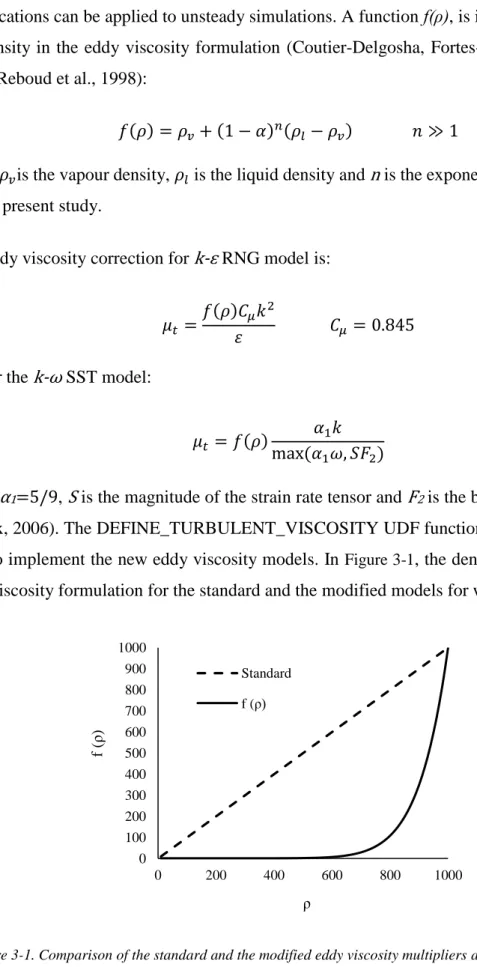
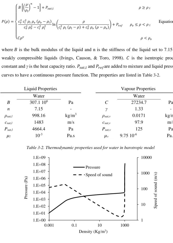
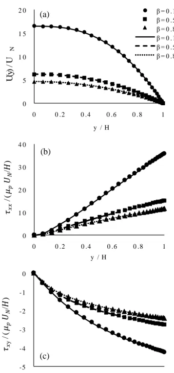
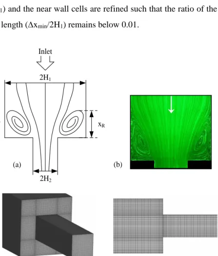
MODELLING OF NOZZLE

CAVITATION IN NEWTONIAN

AND VISCOELASTIC FLUIDS

By Homa Naseri

Thesis Submitted in Partial Fulfillment for

Degree of Doctor of Philosophy

City, University of London, UK

Department of Mechanical Engineering

and Aeronautics

(3)

(4)

II

I, Homa Naseri confirm that the work presented in this thesis is my own. Where information has been derived from other sources, I confirm that this has been indicated in the thesis.

Homa Naseri London, 2019

(5)

III

(6)

IV

Abstract

Cavitation is the abrupt process of vapour formation due to pressure drop in liquid flows, which may occur in various equipment and hydraulic machinery such as propellers, bearings or fuel injectors. In fuel injector nozzles, cavitation formation may be either beneficial or detrimental to the engine performance, depending on the location and type of the vaporous structures. Cavitation can enhance the turbulence levels inside the nozzle and therefore improve the spray atomisation, moreover large vortex cavities known as string cavitation, can increase the spray cone angle. However, cavitation bubbles collapsing near the internal surfaces result in erosion and ultimately failure of the injector parts. Furthermore, excessive vapour formation inside the nozzle significantly reduces the nozzle discharge coefficient and may eventually result in chocked flow conditions. Therefore, understanding the cavitation dynamics and cavitation control is vital for injector design and an active topic in fluid dynamics research.

Newly developed deposit control fuel additives have the potential to reduce the in-nozzle cavitation and enhance the flowrate even in clean injectors due to their non-Newtonian properties. This research aims to provide an understanding about the association between viscoelastic detergent additives and turbulent cavitating nozzle flows using computational fluid dynamics.

An accurate framework for modelling the in-nozzle cavitation is developed. Performance of several RANS and LES models is assessed in predicting incipient and developed cavitation regimes. The Reboud at al. eddy viscosity correction is utilized to compensate the effect of mixture compressibility on turbulent viscosity in k-ɛ RNG and k-ω SST models. WALE LES results are validated against the velocity and rms of turbulent velocity measurements in a step nozzle. A homogeneous equilibrium cavitation model based on Wallis speed of sound formula is utilised to study the effect of vapour-liquid mass transfer rate compared to Zwart-Gerber-Belamri (ZGB) and Schnerr-Sauer (SS) cavitation models. Cavitation vapour fraction values are validated against X-ray CT measurements.

The Phan-Thien-Tanner (PTT) fluid model is implemented to simulate the shear-induced viscoelastic behaviour of Quaternary Ammonium Salt (QAS) surfactants in the additised fuel. The model is validated against analytical solution for channel flow and experimental measurements of corner vortex in a square contraction geometry. The effect of liquid viscosity on cavitation development is presented using LES simulations. Finally, the effect of viscoelasticity on different cavitation regimes, namely cloud cavitation inside a step nozzle and string cavitation in a realistic injector geometry is investigated using LES. The physical flow characteristics are investigated and the effect of the additive on cavitation inside the nozzle is presented. The numerical findings are found to be in agreement with experimental studies of additised fuel.

(7)

V

Acknowledgments

Firstly, I would like to thank my supervisor Prof Manolis Gavaises, for creating the opportunity to conduct this research and for believing in me throughout my journey from an undergraduate student to becoming a PhD. Completing this work would not have been possible without his vision, experience and scientific and financial support. I feel fortunate for the chance to get involved in the work of our research group and to get the opportunity to interact with ambitious researchers in cavitation research.

Secondly, I must thank Dr Ilias Malgarinos for assisting me during the implementation of the CFD code. His help is especially valuable to me as it was during some of the hardest days of my PhD and he supported me with an unbiased attitude and a professional approach.

Furthermore, I would like to thank my advisor Dr Phoevos Koukouvinis for his help in conducting the simulations, sharing his CFD knowledge and experience in processing and publishing the research outcomes. Moreover, the support of my second supervisor Dr Ioannis Karathanassis and our productive discussions on various fluid dynamics topics is also recognised.

Thanks are due to the Lubrizol Corporation, especially Dr Robert Barbour, Dr Kieran Trickett and Dr Eugene Pashkovski, for sharing their knowledge of fuels and additives chemistry, that allowed combining the additive properties in CFD investigations.

I would like to thank all the members of the International Institute for Cavitation Research group at City, University of London. In no particular order, my thanks are to Prof George Bergeles, Prof Jamshid Nouri, Dr Konstantinos Papadopolous, Mr Nikos Chatziarsenis, Dr Hesamaldin Jadidbonab, Dr Nikos Kyriazis, Dr Andreas Papoutsakis, Dr Yves Paquette, Dr Carlos Rodriguez, Ms Georgia Nykteri, Mr Milad Heidari Koochi, Mr Akis Stavropoulos, Mr Alvaro Vidal, Mr Murali-Girija Mithun, Mr Maxwell Brunhart, Mr Thodoris Lyras and Mr Konstantinos Kolovos. I have learnt from each and every person in our group and I am grateful for the nice memories we shared.

I would also like to thank my friends and family for supporting me and being by my side in both sad days and happy days. Thanks to Georgia for being kind and for the precious times that we got to spend together in London and around the university. I also thank Andreea and Khush for growing up with me during our friendship of 7 years, and I thank Soroush, Naimeh, Shahandeh and Magda for being supportive and encouraging throughout my studies.

Special thanks are due to my mother, Dr Saadat Molanaei. I want to thank her for being my inspiration, my best friend in all times and my biggest supporter. Finally, I am grateful to my grandmother, Daye, for her big heart that always had a secure place for me. Without their continuous support and love, I could never reach where I am today or understand the meaning of humanity.

(8)

(9)

VII

Present Contribution

The simulations performed in this thesis provide the following insights:

• Mechanism for “power gain” in additised fuels proposed: This thesis explains the improved volumetric efficiency of fuel injectors enriched with the newly developed deposit control additives containing quaternary ammonium salts. The interaction between viscoelasticity and flow turbulence and cavitation is found to be responsible for the additive effect and the findings are currently employed by the project’s industrial partner, Lubrizol, for developing a new range of additives for enhanced fuel delivery and limiting the pressure losses.

• Flow physics in turbulent and cavitating viscoelastic fluids presented: The Phan-Thien-Tanner model that can simulate the effect of entanglement of surfactant aggregates is implemented in a Navier-Stokes equations flow solver. Instantaneous and time-averaged flow field predictions are analysed to distinguish between the effect of the viscoelastic additives in cloud cavitation and string cavitation in a step nozzle and an injector nozzle. The vapour structures and cavitation cloud shedding dynamics in Newtonian and viscoelastic fluids are compared. To the best of the author’s knowledge, these studies have not been reported in the past.

• Findings consistent with parallel X-ray studies on cavitating flows: The numerical simulations were developed in a close collaboration with experimental studies to identify the additive effect. The conclusions reached regarding the effect of the viscoelasticity on various cavitation regimes are compared with the experiments and the findings are in line with the numerical results.

• Quantitative validation of cavitation vapour fraction: Extent of cavitation predicted in the simulations is validated in detail against X-ray CT measurements of in-nozzle vapour fraction. Quantitative validations for in-nozzle cavitation are scarce in the literature due to the complexity of experimental measurements. The effect of turbulence modelling in cavitation simulation is presented using 2-equation RANS models, RSM model and WALE LES model in a range of cavitation regimes. LES performance in incipient cavitation condition and cloud shedding is validated against experimental data. Effect of mass transfer rate on simulation of turbulent nozzle flow is identified with two-phase mass transfer rate models and the barotropic model.

(10)

(11)

IX

List of figures

Figure 1-1. Microbubble in a liquid at rest ... 3 Figure 1-2. (a) Schematic of nozzle flow and the separated shear layer (b) incipient cavitation (c) developed cavitation (shadowgraphy images (Mauger, Méès, Michard, Azouzi, & Valette, 2012) dark regions indicate the cavitation vapours and grey is the liquid flow) ... 5 Figure 1-3. Flow structures and cavitation vapours in a nozzle, flow structures are presented by means of second invariant of the velocity gradient which identifies the vortex cores (blue translucent iso-surfaces), cavitation structures are presented by the black iso-surface showing regions with 50% liquid and 50% vapour, (1) cavitation inception in the core of microvortices, (2) development of the re-entrant jet instability, (3) shedding of detached cavity cloud ... 6 Figure 1-4. Polyisobutylene polymer made from isobutylene monomers ... 6 Figure 1-5. Flow in a contraction/expansion geometry for (a) Newtonian and (b) viscoelastic fluids at Re  6 (Campo-Deaño & Galindo-Rosales, 2011) ... 7 Figure 1-6. Cross flow geometry and the PIV measurement plane passing through the spiral vortex forming at the junction of the incoming streams (top), Streamlines and PIV measurements of the dimensionless vorticity for (a) water, (b) aqueous solutions of 0.001wt% and (c) 0.003 wt%

polyethylene oxide (Burshtein et al., 2017) ... 8 Figure 1-7. Initially, reverse spherical micelles form, the micelles become cylindrical when salt is introduced in the additive composition and the electrostatic repulsion between the head groups is reduced, cylindrical micelles can entangle and form network microstructures when the fluid is

subjected to shear stress (shear induced structures or SIS) ... 10 Figure 1-8. Direct observation of formation of entangled micellar networks (c) from spherical

micelles (a) by gradually increasing the shear stress (Keller et al., 1998) ... 11 Figure 1-9. The intensity of scattered neutrons versus the scattering vector for the QAS additive blend at different concentrations (symbols) along with the model fits (continuous lines), spherical micelles start forming at concentrations as low as 10 ppm and they start to become elongated at 50 ppm (courtesy of Dr K. Trickett (Naseri et al., 2018))... 14 Figure 1-10. Percentage change of discharge coefficient by addition of the QAS additive at different injection pressures and durations (courtesy of Dr N. Mitroglou (Naseri et al., 2018)) ... 16 Figure 1-11. 3D view of the iso-surface of 50% liquid volume fraction in diesel with 1000 ppm QAS additive (transparent grey colour) and iso-surface of regions with 10% increased liquid volume fraction (αDifference = 0.1, blue colour) (courtesy of Dr N. Mitroglou (Naseri et al., 2018)) ... 17 Figure 1-12. (a) High speed X-ray phase contrast imaging of the cavitation vortex (string) forming under the injector needle,(b) FFT of the string radius fluctuations in base and additised fuels (courtesy of Dr I. Karathanassis (Naseri et al., 2018)) ... 18 Figure 1-13. Appearance of both cloud and string cavitation at higher cavitation number in the XCPI device, (a) the contour of time-averaged probability of vapour presence, (b) Mean cavity surface area

(14)

XII

along the nozzle for the base and the additised fuels, values calculated from the projected vapour area in the mid-plane (image courtesy of Dr I. Karathanassis) ... 19 Figure 2-1: Pressure difference versus mass flow rate for transition of non-cavitating flow to choked flow, CS refers to start of cavitation and CC is the critical cavitation point (Winklhofer et al., 2001) 25 Figure 2-2: Process of cavity shedding, from formation of the re-entrant motion to collapse of the separated bubbles (Sato & Saito, 2002) ... 28 Figure 2-3. Cavitation mechanisms inside a diesel injector nozzle ... 29 Figure 2-4 (a) Cavitation structures in cylindrical (top) and tapered (bottom) injector nozzles; in the cylindrical nozzle a cavity cloud covers the orifice surface area whereas in the tapered nozzle only string cavitation is visible (Gavaises et al., 2009), (b) enhancement of the spray cone angle due to string cavitation presence (Mitroglou et al., 2011) ... 30 Figure 2-5. Shadowgraph of cavitation structures appearing inside an injector replica (left) and X-ray reconstruction of the time-averaged cavitation volume fraction (right) (Mitroglou et al., 2016) ... 31 Figure 2-6. Dynamic behaviour of a string cavitation forming under the needle of an injector replica, white lines show the cavitation interface and images are taken with 1.5 ×10-5 s intervals (I.

Karathanassis, Koukouvinis, Kontolatis, et al., 2017) ... 31 Figure 3-1. Comparison of the standard and the modified eddy viscosity multipliers as a function of density ... 50 Figure 3-2. Graph showing the behaviour of the barotropic EoS and the speed of sound variation as a function of liquid density ... 55 Figure 3-3. Schematic presentation of the velocity profile inside the 2D channel flow ... 58 Figure 3-4. Comparison of the CFD code and the analytical solution for the PTT model;

non-dimensionalized values for (a) the streamwise velocity, (b) normal viscoelastic stresses and (c) tangential viscoelastic stresses are presented in the channel at different viscosity ratios (β = µs/µ0, where µ0 is the total viscosity µp +µs) for ε = 0.25 and De =U/H= 1... 61 Figure 3-5. (a) Schematic representation of the flow in the contraction, (b) streak line photography images showing the corner vortices and the flow path and (c) the computational grid with near-wall refinement for the simulations ... 62 Figure 3-6. Comparison of flow streamline images from the experimental study (green) and the PTT model predictions (grey) for CR 2.4 at different De ... 64 Figure 3-7. Dimensionless corner vortex length at different Deborah numbers for contraction ratios of 2.4 and 4, the results are measured in the centre plane of the contraction geometry ... 64 Figure 3-8. Schematic of the axisymmetric nozzle test section with the main dimensions (all in mm), the flow path is shown using blue arrows ... 66 Figure 3-9. The computational domain and the grid used for the axisymmetric nozzle. (a) the

geometry and flow path (blue arrows), the inlet tubes separated by 120° are demonstrated in the inset, (b) magnified image shows the grid cross-section in more detail ... 66

(15)

XIII

Figure 3-10. Schematic of the asymmetric nozzle geometry and the flow direction (blue arrows), the main dimensions of the nozzle are presented (in mm), for full details of the test section geometry see (Koukouvinis et al., 2017) ... 68 Figure 3-11. (a) The computational domain and the grid used for the asymmetric nozzle, (b)

magnified image shows the grid cross-section in more details ... 69 Figure 3-12. (a) Geometry of the step nozzle and the relevant dimensions in mm, inlet boundary (red color) and outlet boundary (blue color) surfaces are shown; all the other surfaces are no-slip walls (gray color). (b) Computational grid with additional refinement inside the nozzle ... 70 Figure 3-13. (a) Simulation domain for the injector test case. The boundary conditions are indicated by coloured surfaces; inlet and outlet boundaries are coloured in red and blue, respectively, and the green surface shows the periodic boundary (another periodic boundary with the same cross section is located on the opposite side of the geometry); all the other surfaces are no-slip walls (grey colour), (b) The computational grid for the injector; the domain is partitioned using blocking and it is hex-

dominant except from an unstructured tetrahedral section in the sac volume ... 73 Figure 4-1. Photography image of the cavitation cloud forming inside the nozzle for (a) incipient cavitation regime CN = 0.95 and (b) developed cavitation regime CN = 1.5 (Bauer et al., 2012) ... 76 Figure 4-2. Effect of successive grid refinement on pressure distribution inside the cavitating nozzle, the area-averaged pressure values are calculated in several slices along the nozzle ... 76 Figure 4-3. (b) Pressure (b) and streamwise velocity distribution inside the nozzle predicted by the k-ɛ RNG model ... 77 Figure 4-4. Iso-surface of 70% vapour volume fraction artificially introduced at the nozzle inlet (a), cavitation vapours diminish after ~ 1 ms (b) (results predicted by the k-ɛ RNG model) ... 78 Figure 4-5. Time variations of the liquid fraction (solid line) and the turbulence kinetic energy dissipation rate (dashed line) at the nozzle entrance ... 78 Figure 4-6. Iso-surfaces of 70% vapour volume fraction at the nozzle inlet, cavitation vapours

diminish after ~10 ms (results predicted by the k-ω SST model) ... 79 Figure 4-7. Comparison of cavitation distribution inside the nozzle as shown by the experimental image and iso-surfaces of liquid fraction predicted by CFD for the CN = 1.5 condition. In the

simulation results, five translucent iso-surfaces show regions of 5%, 30%, 50%, 70% and 90% liquid fraction ... 80 Figure 4-8. Cross sectional liquid fraction measurement locations along the nozzle are indicated at (a) 4.25 mm, (b) 19.25 mm, (c) 40.25 mm, (d) 59.75 mm, (e) 80.75 mm and (f) 94.25 mm downstream the nozzle entrance, the experimental and numerical values for the liquid fraction are compared side by side. Liquid fraction values higher than 100 represent the solid walls made of Perspex (all values are time-averaged) ... 81 Figure 4-9. (a) Pressure tapping measurements (experiment) and CFD predictions of pressure along the cavitating nozzle length, (b) spatially averaged liquid fraction measured using the X-ray CT and the corresponding predictions by CFD simulations ... 82 Figure 4-10. Distribution of TKE inside the nozzle and the experiment image of the cavitating flow 83

(16)

XIV

Figure 4-11. (a) Shadowgraphy image of the cavitation cloud (Koukouvinis et al., 2017) and (b) translucent iso-surfaces of liquid fraction ranging from 10% to 90%. ... 84 Figure 4-12. Time-averaged contours of liquid fraction in four slices along the nozzle (a) as measured by the X-ray CT experiment and (b) as predicted by RANS simulation ... 85 Figure 4-13. Average liquid fraction values in the nozzle, the experimental X-ray measurements are compared to the numerical predictions and the values are calculated in several slices along the nozzle ... 85 Figure 4-14. (a) Shadowgraphy images of the cavity cloud (b) and iso-surfaces of vapour fraction from the simulations, iso-surface values ranging from 10%-90% at 0.1 ms intervals, green circles in the shadowgraphy images indicate the bubbly cloud regions at the nozzle inlet with a foamy

appearance and red circles show the small-scale vortices shedding from the cloud ... 86 Figure 4-15. Schematic demonstrating the unsteady cavitation cloud structures inside the nozzle (blue colour), the bubbly cloud at the entrance and the small-scale micro-cavities are the major source of discrepancy between the experiments and the CFD results ... 87 Figure 4-16. Effect of grid refinement on streamwise velocity profile predictions at X = 1.5 mm downstream the nozzle entrance (nozzle geometry and measurement location is shown in the inset) . 90 Figure 4-17. Streamwise velocity and RMS of turbulent velocity at three locations downstream the nozzle inlet, experimental data are compared to the standard RANS models ... 92 Figure 4-18. Iso-surface of 50% vapour volume fraction predicted by the modified k-ω SST model, the cavitation vapours completely shed after a few cycles at ~100 µs and the eventually only the liquid phase remains ... 93 Figure 4-19. Iso-surface of 50% vapour volume fraction (left) and contours of TKE in the nozzle midplane (right) as predicted by the modified k-ω SST model, results presented at the begging of the simulation (a) and after ~200 µs (b), black lines show regions below vapour pressure ... 94 Figure 4-20. Streamwise velocity and RMS of turbulent velocity at three locations downstream the nozzle inlet, Experimental data are compared the modified RANS models ... 95 Figure 4-21. Streamwise velocity and RMS of turbulent velocity at three locations downstream the nozzle inlet, results presented for LES simulations with different cavitation models ... 97 Figure 4-22. Indicative (a) pressure and (b) density contours in the nozzle midplane, (c) three

instances of shadowgraphy images showing the in-nozzle vapour distribution in the experimental study (Sou et al., 2014). Black iso-lines in the pressure contour (a) indicate regions where the pressure drops below the saturation pressure and iso-surfaces of 75% liquid fraction are added to the density contours in (b) ... 98 Figure 4-23. Contours of liquid fraction in the midplane of the nozzle predicted by the two-phase models (SS, ZGB and the modified ZGB) and the barotropic model ... 99 Figure 4-24. Instantaneous density contours for (a) standard ZGB model and (b) modified ZGB model at 0.1 ms intervals ... 100 Figure 5-1. Contours of time-averaged velocity (left) and liquid volume fraction (right) in the

(17)

XV

and x0.5) and increased viscosity fluids (by factors x2 and x4), the black iso-lines indicate regions with velocities higher than 18 m/s ... 105 Figure 5-2. Nozzle geometry and cavitation in the shear layer (top), contours of the velocity

magnitude for the Newtonian and the viscoelastic fluid in the mid-plane of the nozzle, the black iso-lines show regions with pressures below the vapour pressure (bottom) ... 106 Figure 5-3. (a) Iso-surface of the second invariant of the velocity gradient with the value 1109_s-2 coloured with the streamwise velocity,(b) 3D view of the iso-surface of the second invariant of the velocity gradient at 3109_s2_{coloured with the streamwise velocity along with iso-surface of 50%} vapour volume fraction (grey colour) ... 107 Figure 5-4. (a) Density variations inside the nozzle during three cavitation cycles, (b) magnitude of the streamwise vorticity, mean values are calculated in several planes along the nozzle length, (c) contour plots of streamwise vorticity inside the nozzle ... 108 Figure 5-5. Energy spectra inside the step nozzle for the Newtonian and the viscoelastic fluid, dashed lines (- - - and - - - - -) show indicative examples of the spectra and continuous lines (⎯ and ⎯) show the mean value of the spectra for the Newtonian and viscoelastic fluid ... 109 Figure 5-6.Comparison of time-averaged values of the streamwise velocity, RMS of streamwise velocity, RMS of wall-normal velocity and Reynolds stress(−𝑢′𝑣′) in the Newtonian and the viscoelastic fluid, data are presented in the mid-plane of the step nozzle at four different X locations along the nozzle ... 110 Figure 5-7.Cavitation development inside the step nozzle presented by means of iso-surfaces of 50 % vapour volume fraction, data are presented every 0.1 ms. Small microcavities shedding from the cloud (blue circle 1) are not present in the viscoelastic fluid, cavitation vapours can initially shrink before growing (red circle 2) and elongated streamwise vortices appear between the detached cloud and the cavitation cloud (red circle 3 and 4) ... 112 Figure 5-8. FFT of mass flowrate fluctuations at the outlet of the step nozzle for the Newtonian and the viscoelastic fluid, the dominant frequency corresponds to frequency of mass flowrate fluctuations induced by cyclic growth and shedding of large cavity clouds ... 113 Figure 5-9. Maximum pressures recorded for the Newtonian (top row) and the viscoelastic fluid (bottom row), images show from the side view (left) and in a 3D view (right) ... 115 Figure 5-10. Time-averaged data for pressure and vapour volume fraction inside the nozzles ... 116 Figure 5-11. (a) Average liquid volume fraction (1-α) in the step nozzle mid-plane along with iso-surfaces of 75%, 80% and 85% average liquid volume fraction in the Newtonian and the viscoelastic fluid, (b) Average liquid volume fraction (1-α) inside the cavitation cloud for the Newtonian and the viscoelastic fluid, values taken along 4 lines passing through the cavitation cloud in the nozzle mid-plane ... 117 Figure 5-12. Pressure spectrum inside the nozzle for the Newtonian and the viscoelastic fluid showing the additive can either increase or decrease the local pressure, depending on t he flow scale (a) Probability of cavitation inception at X = 2 mm for the Newtonian and the viscoelastic fluid (b) ... 118

(18)

XVI

Figure 5-13. (a) Two distinct cavitation regions forming inside the injector nozzle, cavitation vapours are presented using 5 translucent vapour volume fraction iso-surfaces ranging from 0.1 to 1, cavitating vortex is presented by streamlines coloured with pressure, (b) Indicative cavitation structures inside the nozzle at 20 µs intervals (0.1< α <1) showing a larger string cavity in the viscoelastic fluid. ... 119 Figure 5-14. (a) Separated vapour volume fraction regions inside the injector nozzle showing the cloud cavitation and the string cavitation in term of iso-surfaces of 80% vapour volume fraction, (b) Development of the string cavitation (dotted lines • • • • • • and • • • • • • ), the cloud cavitation (dashed lines ⎯ ⎯ and ⎯ ⎯) and the total vapour volume fraction (continuous lines ⎯ and ⎯ ) inside the injector nozzle for the Newtonian and the viscoelastic fluid calculated in several slices along the nozzle axis using area weighted averages, error bars indicate the overlap of the vapour volume fraction in the string and cloud region in 40µm in the vicinity of the nozzle axis,(c)

Normalized helicity (Hn) contours in four slices inside the injector nozzle (at X = 0.2 mm, 0.5 mm, 0.8 mm and 1.1 mm), the black iso-lines show the regions of Hn = 0.95 and Hn→1 in vortex cores ... 120 Figure 5-15. (a) and (b) evaporation and condensations rates computed by the mass transfer rate cavitation model in the cloud and the string cavitation region of the Newtonian and the viscoelastic fluid, (c) vortical flow structures in the vicinity of the injector nozzle entrance plotted using the contours of second invariant of the velocity gradient (Q-criterion) in the nozzle mid-plane and

translucent iso-surfaces of Q-criterion at 5E+12 s-2_{... 122} Figure 5-16. (a) Vortex structures inside the sac volume visualized using the iso-surface of second invariant of the velocity gradient at 4E+12 s-2_{, (b) velocity fluctuations inside the nozzle plotted in} terms of RMS of X,Y and Z velocities, values obtained from surface-averaged data calculated in slices along the nozzle ... 124 Figure 5-17. Schematic representation of the additive effect on the cavitating vortices, black arrows indicate the cavitating vortices and the red arrow shows the axis of rotation of the vortices, cavitation is presented by the blue clouds and the micelles are presented by yellow worms. (a) Cavitating vortices in the recirculation region in the Newtonian fluid (top) and the viscoelastic fluid (bottom), micelles align with the flow and supress vortices rotating out of the nozzle cross sectional plane, (b) Vortex (string) cavitation under the needle in the Newtonian fluid (top) and the viscoelastic fluid (bottom), perturbations by the turbulent eddies can decay the string coherence and breakup the cavitating vortex, micelles can reduce the flow turbulence and contribute to development of a more stable longitudinal vortex and cavity core. ... 125

List of tables

Table 3-1. Thermodynamic properties used for water and diesel in two-phase models ... 54 Table 3-2. Thermodynamic properties used for water in barotropic model... 55 Table 3-3. Test case conditions and the non-dimensional vortex length values measured

experimentally and numerically for contraction ratios 2.4 and 4. Deborah number is defined based on velocity and channel length inside the contraction De =U2/H2. ... 63 Table 3-4. Static pressure values used at the inlet and outlet boundaries for the simulations ... 74 Table 4-1.Grid parameters and their effect on inlet pressure convergence ... 90

(19)

XVII

Glossary of terms

Symbols and abbreviations

B Liquid bulk modulus (Pa)

C Speed of sound (Pa.Kg/m3₎ CFD Computational fluid dynamics

CFL Courant–Friedrichs–Lewy

CN Cavitation number

CR Contraction ratio

DCA Deposit control additive

De Deborah number

EoS Equation of state FFT Fast Fourier transform

Hn Normalized helicity

k Turbulent kinetic energy (m2/s2)

LDV Laser Doppler velocimetry

LES Large eddy simulation

PISO Pressure implicit with splitting of operator

PTT Phan-Thien-Tanner

Pv Vapor pressure (Pa)

Psat Saturation pressure (Pa)

QAS Quaternary ammonium salt

QUICK Quadratic upstream interpolation for convective kinetics R Mass transfer rate (Kg/m3_.s)

ℜB Bubble radius (m)

RANS Reynolds-averaged Navier–Stokes

Re Reynolds number

RMS Root mean square

RNG Renormalization group

RSM Reynolds stress model

S Surface tension (N/m)

SIMPLE Semi-implicit method for pressure-linked equations

(20)

XVIII SST Shear stress transport

St Strouhal number

T Time (s)

tr Tensor trace

UDF User defined function

URANS Unsteady

uτ Friction velocity (m/s)

ZGB Zwart-Gerber-Belamri

WALE Wall-adapting local eddy-viscosity Y+ Dimensionless wall distance

Greek Symbols

IIa Second invariant of the velocity gradient tensor (1/s2)

α Vapour volume fraction

β Viscosity ratio

𝛿_𝑖𝑗 Kronecker delta

𝛾̇ Shear rate (1/s)

 Polymer relaxation time (s) g Taylor length scale (m)

ε Dissipation rate (m2/s3)

φ Probability

µ Dynamic viscosity (Pa.s) µp Polymer viscosity (m2/s) µs Solvent viscosity (m2/s) µt Turbulent viscosity (m2/s) ρ Density (kg/m3) ρl Liquid density (kg/m3) ρv Vapour density (kg/m3) τ Stress (Pa)

τv Viscoelastic stress (Pa) τw Wall shear stress (Pa.s)

υ Kinematic viscosity (m2_/s) ω Specific dissipation rate (1/s)

(21)

(22)

1

1.Introduction

Advances in fuel injection equipment represent a key technology for meeting forthcoming emission regulations and mitigating the environmental impacts by improving fuel economy. As energy demand increases to meet the growing society needs associated with the expansion of urbanisation, population growth and increased car ownership, particularly in developing economies, the CO2 and soot emissions will also escalate. Increasing the fuel injection pressure can reduce the soot emissions; however, it will also increase the amount of cavitation, which can induce material erosion due to bubble collapse inside the injector. In addition, pressurisation of fuel to such extreme levels absorbs a non-negligible amount of useful work produced by the engine. Thus, even small improvements to the rheological characteristics of the fuel can lead to significant energy savings.

Moreover, impurities in the fuel composition may lead to formation of deposit layers on injector parts, altering its internal geometry and significantly blocking the fuel flow. Such effects degrade the injector’s performance, reduce atomisation quality and result in excess and uncontrollable emissions, regardless of the legislation limits the engine met when new (Barker, Richards, Snape, & Meredith, 2011). Injector fouling problems become even more pronounced by large variations of diesel and biodiesel fuel blends. Thus, the use of additives to keep injectors deposit-free is essential for today’s engines. However, due to their proprietary nature, the mechanisms by which the additives affect the injector flow and cavitation are largely missing from the literature.

(23)

2

The current investigation was initiated when it was discovered that some compositions of deposit control additives containing quaternary ammonium salts (R Barbour, 2011) have the ability to increase the volumetric efficiency of clean diesel/biodiesel fuel injectors by up to 5% (Robert Barbour, Quigley, & Panesar, 2014). Further investigations revealed that the main difference between this additive and traditional deposit control additives is formation of elongated micelles which can induce viscoelasticity properties in this fuel composition (I. K. Karathanassis et al., 2018; Naseri et al., 2018).

In this chapter, a brief background regarding the physical characteristics of cavitating nozzle flows and viscoelastic fluids is presented. Furthermore, diesel fuel additives and the role of detergents in the fuel injection systems is discussed. Finally, the research question leading to the current study is presented in the context of previous flow measurements and further X-ray and SANS measurements that were conducted concurrently during this research project.

Cavitation is the phenomenon of vapour formation in flow regions where the local pressure drops below the saturated vapour pressure. The pressure in a liquid flow can drop due to different mechanisms such as flow acceleration, recirculation or pressure oscillations (Brennen, 2013). Phase change can be best described in the context of phase diagrams covering the thermodynamic properties of solid, liquid and gaseous phases. Vapour and liquid can coexist in the dome shaped mixture region between the vapour and the liquid saturation curves. If no nucleation sites are present in the liquid phase (i.e. pure liquid) vapour structures do not form when the fluid is depressurized. At this stage, liquid is under “tension”, where it can withstand negative pressures without phase change and can stay for a certain time in this “metastable” condition. However, in engineering systems, nuclei is always present and phase change occurs at the weak solid-liquid interface. While negative pressures have been found in delicate experiments in liquids (for example see (Brennen, 2013), (Caupin & Stroock, 2013) and (Franc & Michel, 2005)), the existence of such cases in industrial scales is questionable and for water in cavitation tunnels, evidence suggests that pressure in the cavity region matches the saturation pressure (Washio, 2014).

Cavitation can begin from pre-existing microbubbles inside the liquid that grow as the pressure drops. If a microbubble is in equilibrium with the surrounding liquid at rest, pressure inside the

(24)

3

bubble is higher than the surrounding pressure due to the effect of surface tension. Hence, the pressure balance for equilibrium of the interface can be written as:

Pg +Pv = P∞+

2S

R Equation 1.1

where Pg and Pv are pressures of the gas and vapour inside the bubble, P∞ is the surrounding

liquid pressure, S is the surface tension and R is the bubble equilibrium radius. Figure 1-1 shows the schematic of a microbubble inside a liquid and the corresponding pressures.

Figure 1-1. Microbubble in a liquid at rest

As the pressure in the surrounding liquid is reduced, the microbubble expands and the oscillations of the bubble radius are governed by Rayleigh-Plesset equation for bubble dynamics (Plesset, 1949; Rayleigh, 1917):

Rd 2_R dt2 + 3 2( dR dt) 2 +4𝜇𝐿 𝑅 𝑑𝑅 𝑑𝑡 + 2𝑆 𝜌_𝐿𝑅+ Δ𝑃(𝑡) 𝜌_𝐿 = 0 Equation 1.2

where 𝜇𝐿 is the liquid viscosity and 𝜌𝐿 is the liquid density.

Cavitation in a liquid flow occurs when the total stress (pressure plus the deviatoric stress) falls below the vapour pressure (Joseph, 1995). This criterion suggested by Joseph, indicates that cavitation occurs at any point that tension exceeds a threshold, regardless of the values of other principal stresses. Therefore, unlike a liquid at rest where pressure must definitely be below the vapour pressure for cavitation to occur, in a flowing liquid cavitation can happen due to shear stress even when pressure values are above the vapour pressure.

Classical scaling theory implies that the flow regime remains the same when the conditions are scaled up. However due to “scale effects” which arise from changes in the velocity, size, fluid properties and bubbles distribution, this theory does not apply to cavitating flows (Stinebring,

(25)

4

Billet, Lindau, & Kunz, 2001). Scale effects can be divided into two groups; “viscous effects” and “bubble dynamics effects” (Martynov, 2005). Viscous effects make changes in the local pressure field of the liquid surrounding the cavitation bubbles. These include the effects of turbulent pressure fluctuations and geometry imperfections due to surface roughness and manufacturing errors. Bubble dynamics effects have an impact on the behaviour of bubbles formation, growth and collapse. Temperature variations, surface tension, effect of non-condensable gases and micro bubbles in the flow are some of the factors that can affect the bubble dynamics.

Studies of cavitation and bubble dynamics have been the subject of research for more than a century with applications that span across areas such as pumps and turbines, fuel systems and lubricants and biomedical applications. Inside a fuel injector nozzle, cavitation vapours can significantly block the flow passage area and hence reduce the nozzle discharge coefficient. One of the first studies that investigated in-nozzle flow cavitation was carried out by Bergwerk (Bergwerk, 1959) in diesel injector nozzles. This study shows that in non-cavitating flow regimes, the discharge coefficient is mostly a function of the Reynolds number (Re = UD/υ, where U and D are the characteristic velocity and length scale of the flow respectively and υ is the kinematic viscosity). However, in cavitating flow conditions, the cavitation number effect becomes more dominant and therefore cavitating flows are better described by means of cavitation number (see also (D. P. Schmidt, Rutland, & Corradini, 1999b)).

Various formulations are used in the literature to classify cavitation regimes, in the current study, the cavitation number based of the definition proposed by Bergwerk for nozzle flows (Bergwerk, 1959) will be employed:

CN =P1−P2

P₂−Pv

Equation 1.3

where P1 and P2 are the pressure upstream and downstream of the nozzle and Pv is the vapour pressure.

As the flow enters the nozzle, a strong streamline curvature forms due to the sharp turn in the flow direction. This results in the separation of the boundary layer and formation of a recirculation zone at the nozzle entrance, which reduces the cross sectional area for the main flow passage as demonstrated in Figure 1-2. Furthermore, due to the velocity difference

(26)

5

between the recirculating flow and the main flow (VR and VM) a shear layer forms between these two regions that induces further flow instabilities. Cavitation can be induced in the core of microvortices that are produced by the shear layer instability and as the cavitation number is increased, small vapour pockets merge to form larger cavity clouds.

Figure 1-2. (a) Schematic of nozzle flow and the separated shear layer (b) incipient cavitation (c) developed cavitation (shadowgraphy images (Mauger, Méès, Michard, Azouzi, & Valette, 2012), dark regions indicate the

cavitation vapours and grey is the liquid flow)

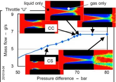
The mass flowrate through the nozzle is a function of the difference between the upstream and downstream pressure (P1 – P2) such that the mass flowrate is enhanced as P is increased. As the cavitation number is increased, vapour structures cover a large area of the nozzle and fill the lower and upper nozzle surfaces. At this point, the mass flowrate reaches a maximum value and it remains constants as P is further increased (choked flow condition) (Mauger et al., 2012; Nurick, 1976).

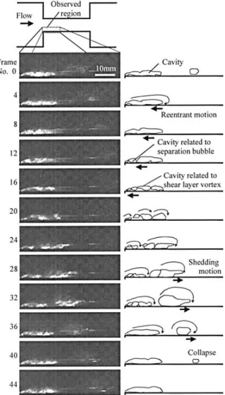
Formation and evolution of cavitation cloud structures is described by a schematic using a simulation instance in Figure 1-3 which shows cavitation development in a step nozzle. Initially, small-scale microcavities appear in the core of the shear layer vortices emerging in the separated flow between the recirculating flow region and the main flow passing through the nozzle (label 1). As these vortices grow and the pressure drops in their core, the size of the cavitation vapours increases and they are convected downstream the nozzle. A re-entrant jet instability (label 2) forms before the cavity closure region due to the adverse pressure gradient in the recirculation region (Callenaere, Franc, Michel, & Riondet, 2001). The re-entrant jet travels upstream toward the nozzle entrance and cuts the liquid/vapour interface, forming a

(a)

(b) (c)

(27)

6

detached cavity cloud. The detached cloud (label 3) is convected towards the nozzle exit by the motion of larger eddies in a turbulent flow region containing a combination of streamwise, spanwise and hairpin vortices (Altimira & Fuchs, 2015). The re-entrant jet instability has a periodic motion that results in cyclic growth and shedding of the cavity cloud. The Strouhal number (St = fL/U, where f is the cloud shedding frequency, L is the cavity length and U is the re-entrant jet velocity) is in the range of 0.2-0.4, irrespective of the operating conditions and the cavity length (Callenaere et al., 2001).

Figure 1-3. Flow structures and cavitation vapours in a nozzle, flow structures are presented by means of second invariant of the velocity gradient which identifies the vortex cores (blue translucent iso-surfaces), cavitation structures are presented by the black iso-surface showing regions with 50% liquid and 50% vapour,

(1) cavitation inception in the core of microvortices, (2) development of the re-entrant jet instability, (3) shedding of detached cavity cloud

More recently, X-ray densitometry of cavitation void fraction in a cavity cloud identified that in addition to the re-entrant jet motion, bubbly shock propagation due to reduction of speed of sound in the liquid/vapour mixture region is also responsible for the shedding of the cavity cloud (Ganesh, Makiharju, & Ceccio, 2016).

Polymers are large molecules made of smaller structural units called monomers. For example, a class of detergents commonly used as fuel additives is amines with a polyisobutylene tail, and polyisobutylene is made from isobutylene monomers:

Figure 1-4. Polyisobutylene polymer made from isobutylene monomers

1 2 3 CH3 CH3 C C H H Isobutylene n CH3 CH3 C C H H Polyisobutylene

(28)

7

The configuration of a polymer can change as it is stretched due to stress or thermal effects and the time scale associated with these changes is known as the “relaxation time”. It is then possible to say that the polymer has a “fading memory” due to the relaxation time required for the polymer to get back to its equilibrium configuration. In Newtonian fluids however, equilibrium state is reached as soon as the stress disappears and the flow is stopped. Polymeric solutions are non-Newtonian and therefore, the shear rate is not linearly proportional to the shear stress. The Non-Newtonian property of viscoelastic fluids is attributed to structural changes or the orientation of particles in the fluid flow. A property of polymeric solutions is that on top of the Newtonian shear stress, they add an extra stress component along the streamline (Bird, Armstrong, Hassager, & Curtiss, 1977). The extra stress is usually measured by means of the “first normal stress difference”, that is the difference between the streamwise stress and the wall-normal stress. The “second normal stress difference” is the difference between the wall-normal and spanwise stresses which has a magnitude much smaller than the first normal stress difference.

In order to characterise the properties of polymeric solutions, various rheological parameters such as storage modulus G′, loss modulus G″, shear viscosity µ, dynamic viscosity η′, polymer viscosity µp and polymer relaxation time λ should be measured at a range of strain rates. Due to the complex behaviour of viscoelastic fluids, it is difficult to define general rheological relations to describe their properties and usually experimental measurements are conducted to define the properties of individual solutions. Extensional viscosity is usually used to define the resistance of viscoelastic fluids when they are subjected to pure extensional (normal) stress and usually polymers with higher molecular weight have higher extensional viscosities and relaxation times.

Figure 1-5. Flow in a contraction/expansion geometry for (a) Newtonian and (b) viscoelastic fluids at Re  6 (Campo-Deaño & Galindo-Rosales, 2011)

(29)

8

The viscoelastic stress effect is observed in many benchmark flow configurations such as the flow around a sphere, rotating disk-cylinder, rising bubble and jet breakup and whether it causes flow stabilization or destabilization largely depends on the specific flow configuration. An example of the additional viscoelastic stresses can be demonstrated in flow near a sudden contraction at low Reynolds numbers (Re  6) in Figure 1-5. In case of the Newtonian fluid, all the flow upstream of the contraction enters the small tube without forming any recirculation zone before the entrance due to the low Reynolds number. However, in the polymeric solution a large recirculation region forms before the entrance. At higher Reynolds numbers corner vortices develop in the Newtonian fluid after the expansion, however in the viscoelastic fluid these corner vortices are completely supressed. (Campo-Deaño & Galindo-Rosales, 2011). This is because in contraction flows, vortex growth is inhibited by increasing the Reynolds number, but the situation is reversed in expansion flows where inertial effects stimulate the vortex growth, likewise the polymer extensional viscosity affects each flow region differently.

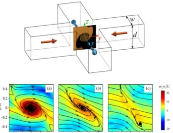
Figure 1-6. Cross flow geometry and the PIV measurement plane passing through the spiral vortex forming at the junction of the incoming streams (top), Streamlines and PIV measurements of the dimensionless vorticity for (a) water, (b) aqueous solutions of 0.001wt% and (c) 0.003 wt% polyethylene oxide (Burshtein, Zografos, Shen,

Poole, & Haward, 2017)

The flow in a pair of cross-slots channels can demonstrate the ability of polymers in supressing the instabilities (Burshtein et al., 2017). The two incoming streams of fluids move in the opposite directions form a spiral vortex core as the flow exists from adjacent channels positioned at 90° with respect to the inlet channels. In Figure 1-6 the flow configuration, streamlines and PIV measurements of vorticity are presented for water and viscoelastic solutions of water and polyethylene oxide. It is evident that by adding polymers and increasing the polymer concentration, the vorticity in the core of the vortex is significantly reduced while

(30)

9

the vortex formation is inhibited. These results indicate that even by adding a very small concentration of high molecular weight polymers to a fluid, the flow instabilities can be supressed by the action of the polymer torque.

It is known that addition of minute amounts of high molecular weight polymers to a solution can reduce the turbulent drag in the flow passing through a pipe. Turbulent drag reduction (DR) by viscoelastic additives is referred to as Toms effect after the first scientist who discovered this property (Toms, 1948). Since then, DR by additives has been studied extensively numerically and experimentally and the knowledge is applied in oil delivery pipelines or district heating/cooling systems to reduce the turbulent drag, heat losses and the pumping costs.

Fuel injectors operate at high injection pressures (>2000 bar) and they have small hole diameters (<0.2 mm) in order to achieve optimum fuel atomization, improve fuel and combustion efficiency and eventually reduce emissions. However, at high temperatures unstable components of the fuel can oxidise and form deposit layers that alter the internal geometry of the injector. Because of the small size of nozzle holes, deposits can significantly block the fuel flow in the injector and reduce the engine efficiency. Additives are blended with diesel fuel in order to improve its properties, they can enhance the performance of the fuel and engine in several ways including:

- Improving the combustion process and reduce emissions - Improving the fuel flow and lubricity

- Removing deposits in the fuel injection system and help engine cleanliness

Diesel fuel injectors are carefully designed, as the injector cleanliness is critical to fuel atomization, mixture formation and subsequently improving combustion efficiency and reduction of fuel consumption and emissions. Deposits formed in tubes of the exhaust gas recirculation system can result in engine knocking and increase NOx emissions and deposit build-up-inside the injector nozzles, results in power loss due to reduction of the fuel flow. Deposit control additives (DCAs or detergents) are usually made of polyalkenyl-succinic-acid derivatives, Mannich bases and ashless polymeric compounds and have a polar head group and a nonpolar tail. The polar head attaches to the deposit precursor and prevents deposit formation

(31)

10

while neutralizing acid activities (dispersant effect/keep-clean effect). A thin layer of additive film covers the metal parts and prevents the formation of new deposit (protective effect). Moreover, the polar head of detergent molecules attaches to deposit layers and removes them from the metal surfaces (clean-up effect). In multifunctional additive packages, deposit control additives are combined with other additives such as antioxidants, antifoam additives, metal deactivators, corrosion inhibitors and cetane improvers (Srivastava & Hancsok, 2014).

As mentioned earlier, polymeric solutions are known for their turbulence suppression properties. Adding small quantities of certain polymers to Newtonian fluids (in some cases as low as a few ppm) induces viscoelastic properties and generally such effects intensify as the polymer concentration increases. For instance, low concentrations of high molecular weight Polyisobutylene (PIB) in oil pipelines are used as drag reducers in treat rates of 10-20 ppm (Mowla & Naderi, 2006). Addition of polymers can alter the dynamics of flow such as laminar to turbulent transition, formation and shedding of vortices and transport of mass, momentum and energy in the flow. Increasing the ratio of counter-ions to surfactants can induce high extensional viscosity, overshoot in normal and shear stress and increase the drag reduction property of viscoelastic fluids. Moreover, viscoelastic surfactant additives are also used in enhanced oil recovery applications to decrease the interfacial surface tension.

Figure 1-7. Initially, reverse spherical micelles form, the micelles become cylindrical when salt is introduced in the additive composition and the electrostatic repulsion between the head groups is reduced, cylindrical micelles can entangle and form network microstructures when the fluid is subjected to shear stress (shear

induced structures or SIS)

Lurizol® diesel fuel deposit control additive compositions can increase the mass flowrate through clean (deposit-free) injection systems, resulting in power gains up to 5% depending on the type of engine (R Barbour, 2011; Robert Barbour et al., 2014). The main novelty of the aforementioned additive is introduction of quaternary ammonium salts to the traditional Polyisobutylene Succinimide (PIBSI) detergent formulation. The flow enhancement effect is attributed to formation of cylindrical micelles by addition of QAS counter-ions to the additive, which can induce viscoelastic properties in the fuel composition.

Spherical micelle Cylindrical micelle Entangled micelle network

(32)

11

urfactant molecules can form spherical micelles as the hydrophobic tail dissolves in the non-polar fuel and the hydrophilic head groups of the surfactant gather in the centre of the micelle (see Figure 1-7). In presence of added salt or electrolytes, surfactant micelles can cluster to form long rodlike micelles that can entangle under shear stress and form network structures. The salt acts by screening the electrostatic repulsion between the charged particles, thus increasing the ionic strength and allowing surfactant molecules to join. When the length of the rodlike micelles increases, they bend and form wormlike micelles (J. Yang, 2002). Figure 1-7 demonstrates the transition of initially spherical micelles to rod-like micelles and finally to entangled networks by addition of salt and shear stress. These network structures are known as shear induced structures (SIS) and can be directly visualised by freeze-fracture electron microscopy (Keller, Boltenhagen, Pine, & Zasadzinski, 1998).

Figure 1-8. Direct observation of formation of entangled micellar networks (c) from spherical micelles (a) by gradually increasing the shear stress (Keller et al., 1998)

Figure 1-8 shows the transition from spherical/rodlike micelle to wormlike micelles and finally entangled micelle networks in a solution of TTAA (tris (2-hydroxyethyl) tallowalkyl ammonium acetate) and NaCl (Keller et al., 1998). Viscoelastic properties can also be present in surfactant solutions where only long rod-like micelles form (i.e. without any evidence of network structures under shear stress).

Due to formation of the rodlike micelles in the fluid, the shear modulus increases and this effect is intensified as the salt concentration increases (Cates & Candau, 1990). However, above a critical micelle concentration, spherical micelles can form again and the viscoelasticity effect is diminished. In linear viscoelastic fluids, either the viscosity or the elasticity property may be dominant depending on the time scale of the experimental measurements. Typically when the experiment time is short and measurements are taken at a fast pace, the elasticity effect becomes more dominant, whereas in longer experimental time scales the viscosity effect can be more significant (Fischer & Rehage, 1997).

(33)

12

Long-chain polymer additives can break under strong shear stress or in high temperatures without returning to their original structure after destruction, and so they lose their viscoelasticity and drag reduction effect. On the other hand, entangled micelle networks in surfactant additives have a more dynamic nature. The main difference in the microstructure between the polymer additives and surfactant additives is that the latter can recombine after breaking, i.e. the surfactant solutions can restore their viscoelastic properties even after breaking. The surfactant networks are in thermodynamic equilibrium with surfactant monomers and molecules are constantly exchanged between the solution and the network, which makes the breaking mechanism reversible. The ability of surfactant additives to self-assemble after breaking renders them beneficial for applications such as fuel injector where the fuel undergoes a lot of shear stress while passing through various parts of the fuel injection equipment and before reaching the injector holes. The high temperatures in diesel injectors can have an adverse effect on the additive effect and reduce the viscoelasticity of the fuel composition. Nonetheless, entangled micelle networks can also demonstrate thermo-thickening properties, i.e. some low viscous micellar solutions become highly viscoelastic by increasing the temperature (Feng, Chu, & Dreiss, 2015), therefore it is necessary to investigate the thermal response of individual solutions to determine their response at high temperatures.

The viscoelastic behaviour of surfactant solutions fits approximately with a Maxwellian fluid model where a damper and a spring in series are used to model the viscoelastic stress. Therefore, the Maxwell fluid model consists of a viscous stress and an elastic stress part:

𝜏 + 𝜕𝜏

𝜕𝑡 = 𝜇0 𝛾̇ Equation 1.4

where τ is the shear stress, 𝜇₀ is the zero shear viscosity,  is the polymer relaxation time and

𝛾̇ is the shear rate . The relaxation time is defined as the ratio of viscosity and the shear modulus

G0 ( = µ0 / G0) (Bird et al., 1977).

However at regions of high shear in entangled polymers, flow properties become non-linear and constitutive equations like Giesekus model (Giesekus, 1982) or Phan-Tien-Tanner model (Thien & Tanner, 1977) are required to describe the flow dynamics. These models are able to predict stress overshoots, non-vanishing second normal stress difference and limiting shear stress at high velocity gradient regions (Fischer & Rehage, 1997).

(34)

13

The current investigation was triggered when some compositions of deposit control additives demonstrated the ability to increase the engine power output above the baseline power, even in clean (deposit-free) injectors (Robert Barbour et al., 2014). Traditional DCAs can clean-up the injector deposits and ideally, return the engine power to the initial value of a deposit-free injector. However the new Lubrizol DCA containing quaternary ammonium salts, can increase the power above the baseline level up to 5% in various engine tests (Robert Barbour et al., 2014), an effect referred to as “power gain” in the original study. The change in the fuel flow

was simultaneously measured, indicating that the specific fuel consumption remained unchanged during the tests. Further investigations that are presented in this section confirm that the increase of power is due to increase of flowrate in the fuel injection system. However, the underlying mechanism for this phenomenon is not understood and describing the power gain

mechanism is challenging as the additive does not significantly alter the physical properties of the fuel such a density and viscosity. Quaternary ammonium surfactants with appropriate counter-ions can be very effective in reducing the turbulent drag in aqueous solutions (Lu et al., 1998), however, less is known about the effect of such surfactants in oil-based solvents or in cavitating flow conditions.

Studies about the interaction of viscoelasticity and cavitating flows are scarce in the literature. A study on tip vortex cavitation in propellers showed that addition of small amounts of high molecular weight polymers in water can delay cavitation inception (Chahine, Frederick, & Bateman, 1993). The effect of viscoelasticity on single bubble dynamics has also been studied experimentally and numerically (E. A. Brujan, Ohl, Lauterborn, & Philipp, 1996a; E A Brujan, 1999; E A Brujan, Ikeda, & Matsumoto, 2004; Dollet, Marmottant, & Garbin, 2018; Fogler & Goddard, 1970; Tanasawa & Yang, 1970; W. Yang & Lawson, 1974). However, there are no studies in the literature investigating the effect of viscoelasticity on turbulent cavitating flows, such as those realised in high-pressure fuel injectors.

This thesis investigates the effect of viscoelasticity on injector flows in a numerical framework and the relevant experimental studies conducted simultaneously by collaborators in the project are also presented in this section. The concurrent studies include small angle neutron scattering (SANS) for investigation of micelles self-assembly in the additive, injector flowrate measurement in tapered and cylindrical nozzles, X-ray micro computed tomography (micro-CT) and high-flux X-ray phase contrast imaging (XPCI) in nozzle replicas to identify the

(35)

14

additive effect in various cavitation regimes. Finally, a hypothesis regarding the effect of the additive on cavitating vortices is developed based on the experimental observations, which will be presented at the end of this section.

Surfactant aggregation properties of the deposit

control additive

SANS studies conducted by Lubrizol provide evidence for the viscoelastic property of the QAS additive (Naseri et al., 2018). The time-of-flight instruments LOQ and SANS2D at the ISIS spallation source located at the Rutherford Appleton Laboratory, UK were used for the SANS experiments.

During spallation, H-_{ions are accelerated and then stripped of their electrons by a thin} aluminium oxide film, producing high energy H+ ions. These ions are further accelerated using a circular synchrotron and then used to bombard a heavy-metal target producing pulses of neutrons which are directed to the sample for the SANS measurements. The observed scattering is dependent on both the wavelength of the incoming radiation and the scattering angle, which can be used to plot the intensity of the scattered neutrons (I(Q)) versus the scattering vector (Q).

Figure 1-9. The intensity of scattered neutrons versus the scattering vector for the QAS additive blend at different concentrations (symbols) along with the model fits (continuous lines), spherical micelles start forming

at concentrations as low as 10 ppm and they start to become elongated at 50 ppm (courtesy of Dr K. Trickett (Naseri et al., 2018)) 0 .0 0 0 0 1 0 .0 0 0 1 0 .0 0 1 0 .0 1 0 .1 1 1 0 1 0 0 0 .0 0 1 0 .0 1 0 .1 1 I(Q ) (c m -1) Q (Å- 1₎ 1 0 0 5 p p m 6 0 3 p p m 3 0 1 p p m 1 0 1 p p m 5 0 p p m 1 0 p p m

(36)

15

The SANS patterns obtained for the PIBSI additive (traditional DCA) fit with a spherical micelle profile with a core radii of 3.5 nm and the shape of the micelles is not concentration dependent; i.e. spherical micelles form in the range of 100 ppm to 14,000 ppm. However, any attempts to fit the QAS additive data with a spherical model is unsuccessful and a cylinder model is used to fit the dataset as shown in Figure 1-9. The QAS additive micelle shape is studied for a wide range of concentrations and it is observed that cylindrical micelles exist in concentrations between 50 ppm to 1,005 ppm. Viscoelasticity has been reported for micelle rod lengths of around 10-40 nm (Ohlendorf, Interthal, & Hoffmann, 1986) and rod lengths of 25-250 nm in concentrations of 100-2,000 ppm (Gyr & Bewersdorff, 2013). The lower end values quoted here are similar to those observed with the QAS additives. It is common for QAS surfactant systems to form highly viscoelastic solutions by forming entangled micelles (Berret, Gamez-Corrales, Séréro, Molino, & Lindner, 2001; In, Bec, Aguerre-Chariol, & Zana, 1999; Oda, Panizza, Schmutz, & Lequeux, 1997) and the viscoelasticity in these solutions is found to be due to formation of three-dimensional dynamic surfactant networks. Likewise, the effectiveness of the additive performance in the highly turbulent and cavitating flow conditions of the injector at such dilute concentrations can be attributed to formation of shear-induced-structures. In fact, a recent Holtzer plot analysis of the additised fuel composition established that the micelles present the morphological characteristics required to form complex network aggregates (I. K. Karathanassis et al., 2018).

Fuel flowrate measurements

Both experimental and computational studies performed in enlarged nozzle replicas (Andriotis, Gavaises, & Arcoumanis, 2008; Gavaises, 2008) have established that nozzles with tapered holes (converging towards the nozzle exit) can supress or eliminate cavitation, although at the highest (>3000 bar) injection pressures, even tapered nozzles are likely to suffer from cavitation. On the other hand, in nozzles with cylindrical holes there is a high level of cavitation and the nozzle discharge coefficient is significantly reduced due to the blockage of the holes by cavitation bubbles (Gavaises, 2008).

The fuel flowrate in cylindrical and tapered injector nozzles in fuel injection equipment is compared in order to determine whether the flow enhancement property of the QAS additive is related to the injector geometry and the amount of in-nozzle cavitation (Naseri et al., 2018). The fuel flowrate is measured by collecting and weighing the injected fuel after 1000 successive injections. The percentage change in the discharge coefficient is calculated from the

(37)

16

difference in the injector flowrate using the base diesel and diesel treated with 1000 ppm of the QAS additive.

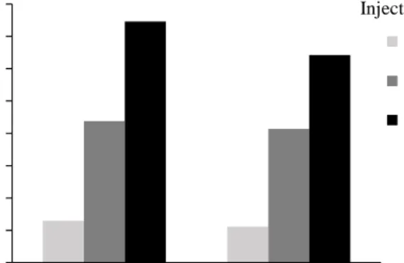
Figure 1-10. Percentage change of discharge coefficient by addition of the QAS additive at different injection pressures and durations (courtesy of Dr N. Mitroglou (Naseri et al., 2018))

It is noted that the additive does not alter the fuel flowrate when tapered injector nozzles are used (only small variations below 0.5% observed in injection pressures from 1300bar to 1800 bar). However, its effect becomes significant in cylindrical nozzles where the flow is more turbulent and prone to cavitation. In cylindrical nozzles, as the injection pressure is increased from 1300 bar to 1800 bar, the discharge coefficient enhancement is also increased from 0.65% to 3.73% for the 1 ms injection duration and from 0.56% to 3.21% for the 1.5 ms injection duration. This observation confirms that the additive is effective in maintaining its flow enhancement property even after passing though the fuel pump, filters and the common rail, providing further evidence about the dynamic nature of the surfactants viscoelasticity. Furthermore, it is demonstrated that the flow enhancement effect is in fact observed in cavitating flow conditions. Moreover, as the injection pressure is increased and so the flow becomes more turbulent and cavitation is enhanced, the additive effect is also improved

Cavitation volume fraction measurements using X-ray

micro-CT

Flow measurement and visualization studies such as shadowgraphy can only provide qualitative information about cavitation. More recently, application of micro-CT (Bauer, Chaves, & Arcoumanis, 2012) and high energy X-rays (Duke et al., 2014; Sun, Jiang, Strzalka, Ocola, & Wang, 2012) have allowed for quantification of cavitation volume fraction. In order to quantify the additive effect on cavitation, a device designed (Mitroglou, Lorenzi, Santini, &

0 0.5 1 1.5 2 2.5 3 3.5 4 1.0 ms 1.5 ms P erc entag e C ha ng e in Dis cha rg e C oe ffic ient Injection Duration 1300 bar 1600 bar 1800 bar Injection Pressure