Aerodynamic optimisation of a camber morphing aerofoil

(1)

Aerodynamic

optimisation

of

a

camber

morphing

aerofoil

J.H.S. Fincham

∗

,

M.I. Friswell

CollegeofEngineering,SwanseaUniversity,SA28PP,UK

a

r

t

i

c

l

e

i

n

f

o

a

b

s

t

r

a

c

t

Articlehistory: Received2October2014

Receivedinrevisedform25February2015 Accepted26February2015

Availableonline3March2015 Keywords:

Morphing Optimisation Multi-objective Geneticalgorithm Radialbasisfunction

Anaircraftthathasbeencarefullyoptimisedforasingleflightconditionwilltendtoperformpoorlyat otherflightconditions.Foraircraftsuchaslong-haulairliners, thisis notnecessarilyaproblem,since thecruiseconditionsoheavilydominatesatypicalmission.However,otheraircraftsuchasUAVs,may beexpectedtoperformwellatawiderangeofflightconditions.Morphingsystemsmaybeasolution tothisproblem,astheyallowtheaircrafttoadaptitsshapetoproduceoptimumperformanceateach flight condition.Optimisationofmorphing aerofoilsis typicallyperformedseparatelytothe morphing mechanismdesign.Inthiswork,anoptimisationstrategyisdevelopedtoaccountforaknownpossible morphing system within the aerodynamic optimisation process itself. This allows for the limitations of the system to be considered from the start of the design process. The Fishbone Active Camber (FishBAC) camber morphing system is chosen as the example mechanism,and it is shown that the FishBACcan achieve large improvementsin performance overnon-morphing aerofoils whenmultiple flight conditionsareconsidered.Additionally,itsperformance iscomparedtoan aerofoilwhose shape canchangearbitrarily(as ifaperfectmorphingmechanismcanbedesigned),anditisshownthatthe FishBACperformsnearlyaswell,despitebeingarelativelysimplemechanism.

1. Introduction

In a broad sense, the camber of an aerofoil describes its asym-metry, and is typically used to control its zero-lift angle of attack. Adding camber, for example, will tend to increase the amount of lift produced at a given angle of attack of the aerofoil, although this is of course limited by stall and separation. There may be changes in the lift to drag ratio also, though with such a broad deﬁnition of camber, it is diﬃcult to state in a general way what this effect will be.

Almost all modern aircraft use discrete control surfaces, such as ﬂaps, ailerons, or sometimes slats, to adjust the camber of the wing. Trailing edge devices are typically hinged surfaces occupy-ing the rearmost 20–30% of the chord which rotate to change their angle, sometimes also translating in the chord-wise direction to increase chord as well as camber. The camber change, however, is almost always discrete in that after actuation of the control surface, there is no longer a smooth transition of camber in the chord-wise direction. This causes a similarly sudden change in the pressure distribution over the corner created at the hinge line, and is associated with a drag penalty and the possibility of separation.

*

Correspondingauthor.

E-mailaddresses:j.h.s.ﬁncham@swansea.ac.uk(J.H.S. Fincham), m.i.friswell@swansea.ac.uk(M.I. Friswell).

While this drag penalty may be deemed acceptable either be-cause the control surface is only used occasionally (such as flaps on an airliner being used only at takeoff or landing), or because there is no suitable alternative, the penalty on surfaces that are in a continuously deflected shape can become significant over a long flight. An example of this would be an elevator or rudder device that is used to trim the vehicle, and is thus being employed for extended periods of time.

Camber-morphing aerofoils aim to achieve their camber change in a smooth way, to potentially reduce this drag penalty. This could be useful in normal aircraft applications, such as the above men-tioned example of a trim-tab or tailplane control surface, but if the problem scope is extended to include rotorcraft, wind turbines, or any number of other applications where aerofoils are required to operate in a wide range of flight conditions, the potential ad-vantages of a camber morphing aerofoil become more apparent. It is at these varied flight conditions that morphing aircraft may be able to provide a significant advantage over traditional aircraft. If the optimum aerodynamic shape is considerably different at the different flight conditions, then it makes sense to have an aircraft whose shape can change on the fly to react to changes in flight conditions, such that it always flies at optimum aerodynamic effi-ciency.

The concept of camber morphing aerofoils is not a new one, and has been extensively studied by engineers over the last hun-dred or so years; an early example is the 1920 design by Parker[1]. http://dx.doi.org/10.1016/j.ast.2015.02.023

(2)

Research activity in this area is even more intense now than it has been in the past, with the general trend being towards compliance rather than mechanism-driven camber changes. Ref.[2]provides a comprehensive review of past and current camber morphing con-cepts.

In traditional aircraft design, aerodynamic and structural design are handled by different groups of engineers, and the design is iterated until an optimum is converged upon. However, morph-ing aircraft design requires tighter integration of the aerodynamic and structural design to ensure that the aerodynamic design pro-duced can be achieved by the morphing systems and structures available. This is a problem that does not appear to be commonly addressed. There are a large number of papers where an aerody-namic analysis is first performed at the different flight conditions, and then a morphing mechanism is produced that can deform the structure to match those desired shapes. Refs. [3–7]are examples of such a design philosophy: the morphing is achieved through compliant mechanisms that can approximately match the target shapes. However, the accuracy to which the external shape can be matched clearly depends upon the complexity and number of de-grees of freedom of the system. A very simple mechanism may only match the target shapes very approximately, whilst a more complex system will match the shapes more accurately, but come at the cost of increased weight (which may very rapidly offset the reduction in drag due to a higher lift-coefficient requirement) and complexity. For example, Gamboa et al. [8]used a complex actu-ation system that can alter the thickness distribution around the chord line in flight, whilst also being able to change the chord length. Despite this, the authors showed that when the flexible skins were considered in an FSI problem, the shapes obtained were still only approximately those obtained from the aerodynamic op-timisation.

In this work, rather than performing an aerodynamic optimi-sation and then designing a morphing system to obtain the re-quired shape-change, the morphing system is explicitly accounted for within the optimiser. This means that the ﬁnal design that the optimiser produces will be directly related to the morphing system in question, effectively turning the problem from multiple single-objective aerodynamic optimisations into a single multi-objective optimisation. The camber morphing system used as an example in this paper is the Fishbone Active Camber (FishBAC) system.

The FishBAC system [9–12] is a biologically inspired compli-ant structure, comprised of a thin bending spine with stringers branching from it. A pretensioned elastomeric matrix composite skin surface provides the aerodynamic shape. The skin tension is used to increase the out-of-plane stiffness, whilst the reinforce-ment is used to produce a near-zero Poisson’s ratio in the spanwise direction. Unlike many other camber morphing designs, the Fish-BAC deformations are achieved purely through compliance of the structure, rather than mechanisms. A non-backdriveable antagonis-tic tendon system is used to drive the deformations.

This work concerns only 2D (aerofoil) optimisation, but the shape-change and optimisation frameworks could be trivially ex-tended to 3D with a suitable aerodynamic analysis tool.

2. Shape-changeframeworkwithradialbasisfunctions

The optimisation tool needs to be able to change the shape of the aerofoil in two ways: ﬁrstly, it must be able to directly modify its external shape (regardless of camber morph) to obtain an opti-mum thickness distribution along the chordline; secondly, it must be able to add the effect of the FishBAC system.

Typically in aerofoil optimisation, the aerofoil is parametrised in some fashion. A common approach is to use a series of splines with control points [8], or to express the aerofoil as a baseline shape plus a summation of shape functions [13]. Spline-based

methods approximate the shape of the aerofoil, and the accuracy of the approximation is dependent upon the number of control points used. Higher degrees of accuracy then imply more degrees of freedom for the optimisation to operate on, which in turn will require longer computational time to reach a converged optimum. These commonly used methods may also not be compatible with an additional camber change, such as the one imposed by Fish-BAC. However, Gamboa et al. [8]had good success using splines to model both an external shape, and a camber morph.

Radial basis function methods [14] are favoured by some au-thors [15–18], especially for FSI simulations where they provide not only a framework to deform the aerodynamic and structural meshes, but a way to interpolate the forces and moments between them, as the two meshes will likely not be coincident. Addition-ally, they extend trivially to three-dimensional problems. A similar approach is used in this work. Using the RBF method, the aero-foil does not need to be parametrised, and is instead expressed as a cloud of points of arbitrary order and spatial resolution. This point cloud is referred to as the aerodynamic surface. A second series of points is used to control the shape of the aerodynamic surface, generally referred to in this work as shape-control points. Again, the order and spatial resolution of these points is arbitrary. Choosing a large number of these shape-control points increases the number of degrees of freedom in the optimisation, giving the opportunity to have more complex shape changes at the cost of increased computational effort. Finally, a third point cloud is used to represent the camber line of the aerofoil, and thus the effect of the morphing actuation system.

These three point clouds are coupled together via matrices, and changes in any one point cloud are interpolated onto the others through these matrices. One of the advantages of the RBF method is that whilst the initial calculation of the coupling matrices re-quires some significant computational effort, once established, the matrices remain constant. If a point cloud changes, then its effect upon the other two point clouds can be calculated by a simple matrix multiplication of the change in the cloud by the relevant coupling matrix. Therefore, once the coupling matrices have been established, all shape changes can be computed with very lit-tle computational cost. The optimisation framework is discussed in more detail in Section 3, but in general terms, the optimiser does not act on the aerodynamic surface cloud directly, but rather modifies the shape-control cloud, which then affects the aerody-namic cloud directly via its coupling matrix. Camber changes occur through the camber cloud, which causes a change in the shape-change cloud, which then in turn changes the external shape to reflect the change in camber.

There are a large number of basis functions to choose from. A radial basis function operates on the radius between points, and returns a scalar value. The returned value will vary between 1.0 when the distance is 0, and 0 when the distance is equal to the support radius. This support radius is chosen by the user, and roughly speaking represents the radius of inﬂuence of one point on the other points. A support radius of just larger than the aero-foil chord length is used in this paper, as this allows all points to affect all others. The Wendland C2 function (shown in Eq.(1)) is selected as the RBF, as it has been used by previous authors with good success [17].

φ (

r

)

=

(

1

−

r

)

4

(

4r

+

1

)

:

0

<

r

≤

1

0

:

1

<

r (1)

Rendall and Allen [17] give a thorough description of the RBF method for FSI problems, and so only a brief summary will be provided here. They commented on the use of polynomial terms in addition to the basis functions to exactly recover rotations and translations. For their work, they used the polynomial terms to

(3)

Fig. 1.Example of a NACA 0012 morphed to different cambers through the RBF method.

calculate the coupling between the structural mesh and the aero-dynamic surface mesh, but did not employ these terms to calculate the coupling between the aerodynamic surface and the CFD vol-ume mesh. This was to prevent the entire mesh from translating or rotating (essentially limiting the deformation in the volume mesh to be near to the wing). In this work, polynomial terms are used for all coupling matrices so that a pure rotation or translation of the surface-control points will produce the same rotation or trans-lation in the camber line and surface, and viceversa.

If the surface-control points were to move by a distance of

xs

(where the subscript s indicates a surface-control point), then the change to the aerodynamic surface (subscript a) is given by:

xa

=

Hsa

xs (2)

The coupling matrix, Hsa, is itself the product of two matrices:

Hsa

=

C−ss1Asa (3)

Css and Asaare calculated as:

Css

=

⎡

⎢

⎣

0 0 0 0 1 1

· · ·

1 0 0 0 0 xs1 xs2

· · ·

xsN 0 0 0 0 ys₁ ys₂

· · ·

ys_N 0 0 0 0 zs1 zs2

· · ·

zsN 1 xs1 ys1 zs1

φ

s1s1

φ

s1s2

· · ·

φ

s1sN

..

.

..

.

..

.

..

.

..

.

..

.

. .

.

..

.

1 xsN ysN zsN

φ

sNs1

φ

sNs2

· · ·

φ

sNsN

⎤

⎥

⎦

(4) Asa

=

⎡

⎢

⎣

1 xa₁ ya₁ za₁

φ

a1s1

φ

a1s2

· · ·

φ

a1sN

..

.

..

.

..

.

..

.

..

.

..

.

. .

.

..

.

1 xaN yaN zaN

φ

aNs1

φ

aNs2

· · ·

φ

aNsN

⎤

⎥

⎦

(5)

Due to the zero-block at the upper left of the Css matrix,

com-putation of the inverse can be performed by extracting the blocks as follows: Css

=

_P0T _MP

(6) C−_ss1

=

MpPM −1 M−1

−

M−1PTMpPM−1

(7) where Mp

=

(

PM−1PT

)

−1 (8)

The process to ﬁnd the other coupling matrices, Hsc(where the

subscript c denotes the camber points) and Hcs can then be

re-peated in an identical fashion.

The choice of spatial resolution of the point clouds depends upon a number of factors. For the aerodynamic cloud, there must

merely be sufficient resolution to produce a smooth shape for the aerodynamic meshing and analysis tool, and there is little penalty in using a large number of points, since the majority of the compu-tational time is likely to be directed towards producing the aero-dynamic solution, rather than calculating the deformed shape of the surface (which as discussed above is a simple matrix multipli-cation). The same can be said for the camber point cloud, which merely needs to be sufficiently fine to accurately represent the camber-line of the aerofoil. Greater resolution of this cloud allows for more complex camber shapes, but since the FishBAC concept used in this paper produces a simple camber morph that is rep-resented to good accuracy with a third order polynomial, only a low resolution of points is required. The polynomial used is shown in Eq.(9), where w is the deflection, and xs is the start location of the morph. Finally, for the shape-control cloud, it is advanta-geous to use as few points as possible, as this will decrease the time required to find the optimum shape. Thus the user will tend to choose the minimum number of points that can still create the range of shapes that may yield optimum performance. Two differ-ent densities of points are used and compared in this work, as it is not known apriorihow many shape-control points are required. w

=

⎧

⎨

⎩

0

:

0

<

x

≤

xs

−

wTE

(

x

−

xs

)

3

(

1

−

xs

)

3

:

xs

<

x (9)

An example of a deformed NACA 0012 aerofoil, showing the effect of a camber change on the surface, is shown in Fig. 1. 3. Optimisationframework

Morphing aircraft usually weigh more than their non-morphing counterparts, on account of their increased mechanism and ac-tuation weight, and also because of their inherent and necessary structural compliance in certain places. This will often lead to strengthening of the structure in other (generally less optimal) places. The vehicles thus make sense when there is a mission with multiple highly varied ﬂight phases, where the optimal shapes are greatly different. For these types of missions, a non-morphing air-craft will be highly compromised in design.

Two different flight conditions are chosen within this work, detailed in Section4. Each has a target lift coefficient, and the ob-jective is to reduce the drag at both flight conditions. Rather than a single optimal aerofoil, there exists a family of aerofoils, all of which may be considered optimum depending upon the relative importance of the two flight conditions. Whilst the optimisation process can go a long way towards automating the aerofoil design, ultimately the decision of which aerofoil is ‘best’ is still up to the aircraft designer, commonly referred to as the decision maker (DM) in optimisation problems.

(4)

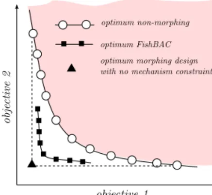
Fig. 2.Examples of non-morphing and morphing Pareto frontiers.

The usual way to represent this family of optimum designs is with a Pareto frontier. In the case chosen here, the two objectives are the drag coefficient at each of the flight conditions. An exam-ple of what the Pareto frontier may look like is shown in Fig. 2. For morphing aerofoil design, previous authors (as mentioned in Sec-tion1) usually approach the problem by producing the Pareto fron-tier, and then attempting to devise a morphing system to morph between two different optimum shapes on the Pareto frontier, e.g. the two designs highlighted at the extremities of Fig. 2(a). This morphing aerofoil will have greater performance at both condi-tions than the ‘best compromise’ aerofoil marked on the figure.

This process, assuming that a perfect morphing system can be achieved, collapses the Pareto population down to a single line, as shown by the grey line in Fig. 2(b), yielding a single optimum individual from the original frontier of Pareto designs (the point on this line closest to the origin). In this work, the goal is to ex-plicitly account for the morphing system within the optimisation itself, such that the ﬁnal aerofoil produced by the optimiser will be achievable by the speciﬁed camber morphing system. Since the limitations of the morphing system are now accounted for, instead of collapsing a non-morphing frontier down to a single line (and thus ultimately a single optimum design), a new Pareto frontier is produced representing a new range of morphing designs. The frontier will generally be smaller than the non-morphing frontier, as the morphing system has effectively reduced the variation in off-design performance of the designs, yielding much closer perfor-mance between all designs on the frontier. However, there will still be a frontier generated rather than a single optimum, and some designs will show better performance in Condition 1 than Condi-tion 2, for example. Because of this, the problem is still treated as a multi-objective optimisation. An example of how this frontier might look is shown in Fig. 3.

Genetic algorithms (GA) are suited to solving multi-objective problems which may exhibit many local optima in design. A GA is used to produce the external shape optimisation of the aero-foils in question. For each individual, when the performance is evaluated at the two flight conditions, a second layer of opti-misation is utilised to determine the best camber morph at the flight condition in question. There are two flight conditions, but each is treated as a single objective optimisation for the morph optimiser. Additionally, the drag as a function of camber morph should be a smooth function, ideally exhibiting a single minimum. A gradient-based optimisation technique should work well for this sub-problem. However, the outer GA optimiser can produce highly unusual aerofoils, especially when morphed, and these will not always produce a converged aerodynamic solution. With the aero-dynamic tool used in this paper, this problem was indeed found to

Fig. 3.Accountingfor themorphing systemintheoptimisationleadstoanew, smaller,frontier.

be the case, and it was deemed simpler and more robust to sim-ply sweep through camber morphs from a prescribed minimum to maximum, whilst discarding non-converged or spurious results. The minimum can then be selected, and refinement of the step-size performed in the area of interest, if required. This is a simple technique which is likely not the most efficient, but is at least ro-bust. It should be noted that changing camber also causes a change in lift coefficient at a given angle of attack, so the correct

α

value must be computed for each new morph to obtain the desired CL. The operations within one generation of the GA are summarised in Fig. 4.

A relatively standard GA technique is used within this paper. The only non-standard addition is a variable mutation rate to pro-mote diversity within small populations. A linear function is used that scales the rate of mutation from a high level for small pop-ulations, and a low baseline level when the breeding population reaches a certain size.

4. Softwareandproblemdeﬁnition

The GA and camber-morphing optimisation are written in Python, whilst the aerodynamic solver used is XFOIL, a 2D panel method with coupled boundary layer solver [19]. XFOIL has shown good performance when compared to RANS CFD for this speciﬁc type of problem [12], and can simulate the effects of transition, separation, and compressibility, all to varying degrees of approxi-mation. Compared with RANS methods, the solution time is orders of magnitude lower. The optimisation algorithm is trivially paral-lelisable (with close to linear speed-up), and so is run on 10 cores in this work.

(5)

Fig. 4.Order of operations for performance evaluation for a given population.

Table 1

Flightconditionsconsidered.

Reynolds number Mach CL

Condition 1 6.5E+05 0.100 0.800

Condition 2 2.5E+06 0.417 0.046

Two ﬂight conditions are considered, which are summarised in Table 1. The low Reynolds number case can be considered a loiter case, whilst the high Reynolds number case is considered to be a dash or cruise case. These ﬂight conditions may be typical of a military UAV, which would dash to an area, and then loiter to perform reconnaissance.

The optimisation problem as described in Section 3is consid-ered. A non-morphing case is also considered so that the advan-tage of a morphing aerofoil can be compared to that of a compro-mised non-morphing aerofoil.

Through the RBF method, each individual within the popula-tion is expressed as a set of perturbations from a baseline shape. Choosing a good starting shape is important, as it will greatly speed up the convergence to the optimum set of solutions. Since a camber morph is allowed for in the problem described in Sec-tion3, it is expected that the external shape of the aerofoil may not need to be signiﬁcantly cambered. Because of this expectation, the NACA 0012 aerofoil is selected as a baseline, as it is a symmet-ric aerofoil that is known to have reasonably good performance at low Mach numbers.

The two optimisation processes (non-morphing and morphing) are both repeated for two sets of surface-control points. It was briefly mentioned in Section2that the number of surface-control points required is unknown before performing the optimisation to obtain the best set of optimum designs. In the first set, referred to as Set A, and shown in Fig. 5, six control points are used. The leading edge point is not allowed to move, whilst the trailing edge point is only allowed to move in the z(vertical) direction, to effec-tively fix the chord-length of the aerofoil. It is worth noting here that for a real camber-morphing aerofoil, the chord length will shorten as the aerofoil is deflected. However, this shortening effect has previously been shown to be small, even for very large deflec-tions, and can thus be ignored [20]. The other four control points (two on the upper surface, and two on the lower) all have two degrees of freedom, and so are free to translate in both x and z. The upstream of these two are bounded between 0

<

x

≤

0

.

5 and the downstream two points are bounded so that 0

.

5c

<

x

≤

1

.

0. In terms of z bounds, the upper two points are bounded so that 0

<

z

≤

0

.

1, whilst the lower two points are bounded between 0

>

z

≥ −

0

.

1. Although these bounds effectively permit an aerofoil of zero thickness, the optimiser does not generally run up against this constraint, and will be shown to often choose a thinner aero-foil than the NACA 0012 baseline. A very thin wing will have its own structural issues which are not considered in this work, but could be incorporated within the problem constraints. The total number of degrees of freedom for the outer shape is thus 9, ex-cluding the ability to camber morph, which could be considered as an additional degree of freedom.

Fig. 5.The two sets of surface-control points used.

The first set of surface-control points discussed above allows for some control over the total thickness of the aerofoil, as well as the position of maximum thickness, with some control, albeit lim-ited, over the aerofoil camber. The position of maximum thickness, however, is not explicitly controlled, and is inherently a function of the positions of the upstream and downstream surface-control points. The second set (B) of control points used includes an addi-tional two points located at the position of maximum thickness of the baseline aerofoil, as shown in Fig. 5. This gives greater control over the position of maximum thickness, as well as the thick-ness to chord ratio, whilst also independently allowing for concave shapes, such as those typically found in reflex or supercritical aero-foils. It is not expected that a great degree of concavity will be required in this work to reach an optimum, but it is useful to con-sider this possibility. If the problem suited reflex or supercritical aerofoils more (such as a requirement to carefully control pitch-ing moment, or for transonic cases), surface-control points such as Set B may be required. The number of degrees of freedom for Set B is 13, excluding the camber morphing ability.

5. Resultsanddiscussion

Before optimisation of the morphing aerofoil was performed, the non-morphing case was computed. This serves as a useful comparison, not only because it will help to quantify the advan-tage of morphing aerofoils vs. their non-morphing counterparts, but also because it is the method used to optimise aerofoils that can morph arbitrarily (and thus shadows the work of previous au-thors).

Fig. 6shows the ﬁnal-generation populations and Pareto fronts from the optimisations. The green and red points show the two sets of non-morphing Pareto frontiers. The two sets of results share the same trends at end points of the frontier (representing the best aerofoils for a single condition only), and general shape and slope of the frontier. For the most part, the frontier is approximately a straight line, indicating a simple trade-off between performance in Condition 1 and Condition 2. The slope is an important parameter because it indicates the penalty in designing for off-design condi-tions. There is a corner produced at good Condition 1 performance (upper left on the graph), but a relatively short arm of the frontier above this in both Set A and Set B results.

Set B shows consistently better performance across the frontier, however, which demonstrates that a greater performance can be achieved by allowing for a larger number of degrees of freedom

(6)

Fig. 6.Populations from the optimisations.

within the shape optimiser. However, one can expect that adding additional degrees of freedom beyond Set B will yield diminish-ing returns at greater computational cost to reach an optimum set of designs. Genetic algorithms are usually run multiple times since they rely on a stochastic search of the design space. For these re-sults, and especially those in Set B, populations from different runs were merged together in an attempt to provide a more even cov-erage of the Pareto frontier. It is a common problem with GA that without using this merging technique, the frontier from any sin-gle run is unlikely to be free of significant gaps. Unfortunately, by doing this, convergence is difficult to track, and so no convergence data is provided in this work. However, it can be safely said that Set B populations took significantly more computational effort to reach a satisfactory (both converged and without gaps) frontier.

Several aerofoils from the Pareto frontiers are compared in Ta-ble 2. For each of Set A and Set B, three aerofoils are chosen representing: the best aerofoil in Condition 1; the best aerofoil in Condition 2; and the ‘best compromise’ aerofoil. In this case, the best compromise aerofoil is considered to be the one that is the minimum distance from the origin in the objective function space (Fig. 6), effectively placing equal importance on the two ﬂight con-ditions. As was discussed previously, Set A and Set B performance is very similar. Choosing the best aerofoils for Condition 1 shows that drag from the baseline aerofoil (NACA 0012) can be reduced by over 50% in Condition 1, at the expense of increased drag in Condition 2 (13% for Set A, and 17% for Set B). For the Condi-tion 2 aerofoils, the opposite is true; performance in Condition 1 has been traded off (approximately a 12% increase in drag for both sets) to achieve a signiﬁcant reduction in drag in Condition 2 (36% for Set A, and 39% for Set B). The best compromise aerofoils are both reasonably close in performance to their Condition 1 coun-terparts. However, the drag at Condition 2 is actually higher than that of the baseline aerofoil. Condition 2 has a very low target CL to represent a high-speed dash condition. This favours symmetrical aerofoil designs, but in order to obtain performance in Condition 1, the best compromise aerofoils tend to be slightly cambered.

The generally poor performance of the baseline aerofoil can be attributed to its ‘peaky’ pressure distribution, in which the suction peak is located very near to the leading edge, and shows a large unfavourable gradient on the upper surface shortly thereafter. This causes a relatively early laminar–turbulent transition of the

bound-Table 2

Comparisonofdragforvariousnon-morphingaerofoils.

Best in Condition 1 Best in Condition 2 Best compromise CD1 CD2 CD1 CD2 CD1 CD2

Set A 0.00559 0.00617 0.01386 0.00347 0.00574 0.00578

Set B 0.00544 0.00640 0.01335 0.00335 0.00565 0.00566

Baseline aerofoil (NACA 0012) CD1 CD2

0.12080 0.00545

Table 3

Transitionpointsforvariousnon-morphingaerofoils.

Condition 1 Condition 2

Upperxtr Lowerxtr Upperxtr Lowerxtr

Best in Condition 1 Set A 0.7616 1.000 0.8575 0.0360 Set B 0.7706 1.000 0.8716 0.0150 Best in Condition 2 Set A 0.0175 1.000 0.7928 0.7341 Set B 0.0196 0.9975 0.7642 0.7761 Best compromise Set A 0.7163 1.000 0.8511 0.0961 Set B 0.7636 0.9995 0.8703 0.1093

Baseline aerofoil (NACA 0012)

0.0650 0.9959 0.4671 0.5438

ary layer, leading to higher drag. Since XFOIL has been set up to calculate transition, the optimiser is generally driving the designs towards natural laminar ﬂow. This can be seen in Table 3, which shows the transition position (normalised by chord length) on the upper and lower surfaces of three aerofoils of interest from each set.

The table shows that the baseline aerofoil transitions very near to the leading edge on the upper side in Condition 1. The best aerofoils in Condition 1 from Set A and Set B show that this tran-sition point has been moved back to a little further than 75% chord, which is associated with the signiﬁcantly lower drag value, shown in Table 2. The best aerofoils in Condition 2, however, show even less laminar ﬂow than the baseline at Condition 1. Unsur-prisingly, they show much better transition performance at

(7)

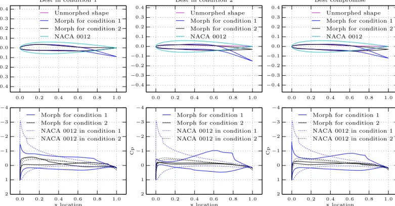
Con-Fig. 7.Non-morphingaerofoilperformance(SetAonleft,SetBonright),showingthebestaerofoilineachﬂightcondition,plusthebestcompromisebetweenthetwo,in additiontoabaselineNACA0012.(Forinterpretationofthereferencestocolourinthisﬁgure,thereaderisreferredtothewebversionofthisarticle.)

dition 2, where the baseline aerofoil transitions at around 45–55% on both upper and lower surface, whilst both Set A and B opti-mised aerofoils transition at between 70 and 80%. Finally, the best compromise aerofoils show very similar transition performance to the best aerofoils in Condition 1 at Condition 1, but tend to lose their laminar ﬂow over the lower surface in Condition 2, unlike the baseline aerofoil – this can be directly related to their increase in drag over the baseline aerofoil in Condition 2.

Fig. 7shows the shape and pressure distribution of the three aerofoils from each set. Due to the relatively short length of the upper arm of the Pareto front in Fig. 6, the best compromise aero-foil is similar in shape to the best aeroaero-foil in Condition 1 for both sets of control points. This is reﬂected in the pressure distribution plots, which show that for both sets of aerofoils at Condition 1, the best aerofoil and the compromise aerofoil have reduced suction peaks from the baseline aerofoil (and the best aerofoil for

(8)

Condi-Fig. 8.Relative performance of morphing vs. non-morphing aerofoils as a function ofCDin ﬂight conditions 1 and 2, for Set A.

tion 2). In Condition 2, both sets of aerofoils show that the best at Condition 1 now displays a large suction peak at the leading edge, whilst the compromise, best, and baseline aerofoils all show a reduction in the suction peak and correspondingly higher perfor-mance.

The blue line represents the best aerofoil at Condition 2, and shows how the optimiser has attempted to flatten the pressure distribution to produce a very small amount of lift. The moment coefficient is not constrained or penalised within this work, but it is worth noting that some aerofoils show the upper and lower pressure lines crossing in Condition 2. This might suggest that a large moment coefficient is being generated in these cases, which might not be a favourable characteristic. To avoid this, one could incorporate a simple constraint within the optimiser (valid individ-uals must have a moment coefficient smaller in magnitude than a certain value), or as an additional objective (minimise both drag and moment) at considerably increased computational cost.

Returning to Fig. 6, the improvement in performance for the FishBAC aerofoils over the non-morphing aerofoils can be clearly seen by the movement of the Pareto frontier towards the ori-gin. As predicted in Section 3, the frontiers are smaller than the non-morphing frontiers, and exhibit a sharper corner, making the choice of ‘best compromise’ aerofoil a little clearer. Again, Set B has slightly out-performed Set A, although the general shape and end-points of the frontiers are very similar. The morphing aero-foils appear to have reached a better optimum at Condition 2 than the non-morphing optimisation found, which indicates that the non-morphing optimisations have yet to successfully identify the end-point of the frontier.

The relative performance of the morphing aerofoils to the non-morphing frontiers is shown for Set A in Fig. 8; Set B results are not shown, but display a similar trend. The left-hand subfigure shows the drag in Condition 2 for a given drag in Condition 1, whilst the right-hand subfigure shows the opposite. These figures essentially show the benefit of morphing in off-design conditions; for a given required performance in the main flight condition, they show the benefit in the off-design condition. From the left-hand figure, the morphing aerofoil is producing approximately 30–45% less drag in Condition 2 for any given desired performance in Con-dition 1. From the right-hand subfigure, at a given performance in Condition 2, the morphing aerofoils perform 50% to 58% bet-ter in Condition 1. The main difference between these two figures (which show two interpretations of the same data) is that if Con-dition 1 is considered to be the main condition, as the design moves towards higher performance in this condition, the

mor-phing and non-morphing aerofoil performance grows closer. In Condition 2, however, the opposite is true; the morphing aero-foil becomes ever better as greater performance in Condition 2 is required. These ﬁgures begin to highlight some of the issues a designer may face when attempting to decide if morphing con-cepts are worthwhile on his or her aircraft. There is a complex trade study required. Even though the morphing designs show at worst 30% less drag than non-morphing, there is of course an un-modelled weight penalty associated with morphing systems that should be accounted for, so the true morphing vs. non-morphing comparison will be rather more complex than this.

Figs. 9 and10show the shapes of three aerofoils from the two morphing Pareto fronts (Set A and Set B). Firstly, there is less varia-tion between the three designs within each set than has been seen previously. The ability to morph has reduced the size of the Pareto frontier, but has also reduced the variation in shapes required to produce it. The optimiser has generally found thin shapes – this is slightly more pronounced than for the non-morphing aerofoils, which tended to be thinner than the baseline design, but not to an extreme extent. It may be necessary for a designer to place stricter bounds on the minimum thickness than has been done here, to ensure that a suitable structure can be designed.

Both ﬁgures plot three shapes for each individual design: the shape at each of the two ﬂight conditions, in addition to an un-morphed shape. It is this unmorphed shape that the optimiser acts upon. Although not constrained to do so, it has generally cho-sen reasonably symmetric designs, and then utilised the FishBAC mechanism to add the camber required for optimum performance in Condition 1, and to a lesser extent, Condition 2. To make clear the shape-change due to FishBAC, the plots show the geometric shapes of the aerofoils, rather than plotting them at their correct angle of attack.

The pressure distributions show the same trends as those seen for the non-morphing aerofoils. The optimiser has tried to reduce the peakiness of the pressure distribution to encourage laminar ﬂow, whilst those aerofoils that perform well in Condition 2 have very ﬂat pressure distributions. Set A and Set B show the same trends in shapes and pressure distributions.

Finally, it is worth considering the performance of the opti-mised FishBAC aerofoil against that of an aerofoil with an arbitrary or perfect morphing mechanism. This aerofoil will have the perfor-mance of the best non-morphing aerofoils for Conditions 1 and 2, and is compared to the FishBAC and the baseline aerofoil in Ta-ble 4. Despite the relatively simple mechanism of the FishBAC, which can change camber only, careful tailoring of the thickness

(9)

Fig. 9.Morphingaerofoilperformance(SetA),showingthebestaerofoilineachﬂightcondition,plusthebestcompromisebetweenthetwo,inadditiontoabaselineNACA 0012.

Fig. 10.Morphingaerofoilperformance(Set B),showingthebestaerofoilineachﬂightcondition,plusthebestcompromisebetweenthetwo,inadditiontoabaselineNACA 0012.

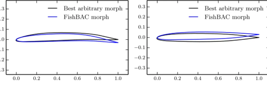
distribution around the camber line means that the drag is only 3.5% higher at Condition 1, and 2.4% higher at Condition 2 than the aerofoil which can change shape arbitrarily. Relative to the base-line aerofoil, there is still a very large increase in performance, but without the necessity to design a complex (and possibly heavy) mechanism as would be the case for the arbitrarily morphing aero-foil. Fig. 11shows that the optimum FishBAC aerofoil is very close in shape to the optimum arbitrary morphing aerofoil.

Table 4

FishBACperformancevs.thebaselineaerofoilandanarbitrarymorphingaerofoil.

CD1 CD2

NACA 0012 0.12080 0.00545

Best compromise FishBAC 0.00563 0.00343

(10)

Fig. 11.Optimum FishBAC shapes compared to the optimum shapes for an arbitrary morphing aerofoil.

6. Conclusions

A multi-objective optimisation method for morphing aerofoils has been designed with the intention to incorporate specific mor-phing systems into the optimisation process, rather than design-ing the morphing systems and aerofoils separately. The FishBAC camber-morphing concept was used as the morphing system. In order to perform the optimisation, two different optimisation tech-niques were coupled together: the first to optimise the thickness distribution of the aerofoil, and the second to find the optimum amount of camber to add for each objective. A Pareto frontier of optimum designs was produced. This differs from the conven-tional approach, where the aerofoils are optimised without consid-eration of morphing capability, and then a morphing mechanism is designed to attempt to morph between the best shapes. This approach yields only a single optimum design, but can lead to highly complex morphing mechanisms required to match the tar-get shapes.

Both the thickness distribution and camber morph were applied to the baseline design via radial basis function interpolation, which allows for smooth shape changes with any number of degrees of freedom, without the need to parametrise aerofoil shape via shape functions or splines. This method is computationally eﬃcient, and easy to work with, since it acts upon unstructured clouds of points. Three clouds of points (aerodynamic surface, shape control, and camberline points) were coupled together within the RBF frame-work through simple coupling matrices.

Two different sets of surface-control points have been studied, with differing degrees of freedom, since it is unknown apriori how many are required to reach a satisfactory optimum design. Ultimately, it has been shown that there is a small beneﬁt for in-creasing the number of degrees of freedom, though it is expected that increasing this further will yield diminishing returns at the cost of greater computational expense.

Pareto frontiers for the two sets of points were generated for non-morphing aerofoils via a genetic algorithm. When the coupled optimiser was applied to the FishBAC, it was found that there was a very large improvement in performance obtained by having a morphing aerofoil. For matched performance in on-design condi-tions, the drag reduction in off-design conditions varied from 30% to almost 60%.

When compared to an aerofoil which can morph arbitrarily (an assumed perfect morphing system that can change to any shape), the FishBAC was found to have 2–4% more drag. However, consid-ering the simplicity of the morphing mechanism, this is considered a very promising result; nearly the same performance as a perfect system was obtained simply through a single degree of freedom camber morph (FishBAC), plus careful tailoring of the thickness distribution.

Conﬂictofintereststatement

We wish to conﬁrm that there are no known conﬂicts of in-terest associated with this publication and that the only source of

ﬁnancial support has come from the European Research Council, which has not inﬂuenced the outcome of the work.

We confirm that the manuscript has been read and approved by all named authors and that there are no other persons who satisfied the criteria for authorship but are not listed. We further confirm that the order of authors listed in the manuscript has been approved by all of us.

We conﬁrm that we have given due consideration to the pro-tection of intellectual property associated with this work and that there are no impediments to publication, including the timing of publication, with respect to intellectual property. In so doing we conﬁrm that we have followed the regulations of our institutions concerning intellectual property.

We understand that the Corresponding Author is the sole con-tact for the Editorial process (including Editorial Manager and di-rect communications with the office). He/she is responsible for communicating with the other authors about progress, submis-sions of revisions and final approval of proofs. We confirm that we have provided a current, correct email address which is acces-sible by the Corresponding Author and which has been configured to accept email from j.h.s.fincham@swansea.ac.uk.

Acknowledgements

The research leading to these results has received funding from the European Research Council under the European Union’s Sev-enth Framework Programme (FP/2007–2013)/ERC Grant Agreement No. (247045).

References

[1]H.F.Parker,TheParkervariablecamberwing,TechnicalReportNo.77,NACA, 1920.

[2]S.Barbarino,O.Bilgen,R.M.Ajaj,M.I.Friswell,D.J.Inman,Areviewof morph-ingaircraft,J.Intell.Mater.Syst.Struct.22(June2011)823–877.

[3] E.Gillebaart,RoelanddeBreuker,Optimisationofamechanicallinkagefora morphingwinglet,in:Proceedingsofthe DeMEASSVIConference, Ede,The Netherlands,May2014.

[4] M.Radestock,J.Riemenschneider,H.P.Monner, M.Rose,Structural optimiza-tionofanUAVleadingedgewithtopologyoptimization,in:Proceedingsofthe DeMEASSVIConference,Ede,TheNetherlands,May2014.

[5] J.Sodja,RoelanddeBreuker,M.Martinez,Geometryandforcevalidationof themorphingleadingedgeconcept,in:ProceedingsoftheDeMEASSVI Con-ference,Ede,TheNetherlands,May2014.

[6]J.J.Joo,G.W.Reich,J.T.Westfall,Flexibleskindevelopmentformorphingaircraft applicationsviatopologyoptimisation,J.Intell.Mater.Syst.Struct.20 (Novem-ber2009)1969–1985.

[7] D.Baker,M.I.Friswell,Thedesignofmorphingaerofoilsusingcompliant mech-anisms,in:The19thInternationalConferenceonAdaptiveStructuresand Tech-nologies,Ascona,Switzerland,October2008.

[8]P.Gamboa,J.Vale, F.J.P.Lau,A.Suleman,Optimizationofamorphingwing based on coupled aerodynamic and structural constraints, AIAA J. 47 (9) (September2009)2087–2103.

[9] B.K.S.Woods,M.I.Friswell,Preliminaryinvestigationofaﬁshboneactive cam-berconcept,in:ProceedingsoftheASME2012ConferenceonSmartMaterials, AdaptiveStructuresandIntelligentSystems,Stone Mountain,GA,September 19–21,2012.

(11)

[13]S.Eyi,J.O.Hager,K.D.Lee,AirfoildesignoptimizationusingtheNavier–Stokes equations,J.Optim.TheoryAppl.83 (3)(December1994)447–461.

[14]H.Wendland,ScatteredDataApproximation,CambridgeUniversityPress,2005. [15]R.Ahrem,A.Beckert,H.Wendland,Ameshless spatialcouplingschemefor large-scaleﬂuid–structureinteractionproblems,Comput.Model.Eng.Sci.12 (2006)121–136.

tion,Int.J.Numer.MethodsFluids58(March2008)827–860.

[19]M. Drela, XFOIL: an analysis and design system of low Reynolds number aerofoils, in:Low ReynoldsNumber Aerodynamics,vol. 54, Springer-Verlag, 1989.

[20]B.K.S.Woods,I.Dayyani,M.I.Friswell,Fluid/structure-interactionanalysisofthe ﬁsh-bone-active-cambermorphingconcept,J.Aircr.52 (1)(2015)307–319.