Hypersonic Transition Analysis for HIFiRE Experiments
Fei Li,* Meelan Choudhari,* Chau-Lyan Chang* NASA Langley Research Center, Hampton, VA 23681
Roger Kimmel# and David Adamczak& Air Force Research Laboratory, WPAFB, OH 45433
Mark Smith##
NASA Dryden Flight Research Center, Edwards, CA 93523 Abstract
The HIFiRE-1 flight experiment provided a valuable database pertaining to boundary layer transition over a 7-degree half-angle, circular cone model from supersonic to hypersonic Mach numbers, and a range of Reynolds numbers and angles of attack. This paper reports selected findings from the ongoing computational analysis of the measured in-flight transition behavior. Transition during the ascent phase at nearly zero degree angle of attack is dominated by second mode instabilities except in the vicinity of the cone meridian where a roughness element was placed midway along the length of the cone. The growth of first mode instabilities is found to be weak at all trajectory points analyzed from the ascent phase. For times less than approximately 18.5 seconds into the flight, the peak amplification ratio for second mode disturbances is sufficiently small because of the lower Mach numbers at earlier times, so that the transition behavior inferred from the measurements is attributed to an unknown physical mechanism, potentially related to step discontinuities in surface height near the locations of a change in the surface material. Based on the time histories of temperature and/or heat flux at transducer locations within the aft portion of the cone, the onset of transition correlated with a linear N-factor, based on parabolized stability equations, of approximately 13. Due to the large angles of attack during the re-entry phase, crossflow instability may play a significant role in transition. Computations also indicate the presence of pronounced crossflow separation over a significant portion of the trajectory segment that is relevant to transition analysis.
Nomenclature
f = frequency of instability waves M∞ = freestream Mach number n = azimuthal wavenumber P∞ = freestream pressure
Re = freestream unit Reynolds number
Ren = Reynolds number based on nose radius and free-stream conditions s = surface distance
t = time elapsed since the start of the flight experiment Tw = wall temperature
T∞ = freestream temperature N = N-factor of linear instabilities U = axial velocity component Uc = crossflow velocity component Ue = axial velocity at boundary layer edge Un = wall-normal velocity component Us = streamwise velocity component X = axial coordinate
*
Aerospace Technologist, Computational AeroSciences Branch, M.S. 128. #
Senior Research Engineer, Air Vehicle Directorate, 2130 8th St &
Senior Aerospace Engineer, Air Vehicle Directorate, 2130 8th St. ##
Aerospace Engineer, Aerodynamics and Propulsion Branch, M.S. 2228. Hypersonic Laminar-Turbulent Transition Meeting,
San Diego, California, April 16-19, 2012.
Xtr = axial coordinate of transition location
y = Cartesian coordinate orthogonal to cone axis within symmetry plane Y = wall-normal coordinate
α = angle of attack (degrees) ν = angle of attack (degrees)
θ = azimuthal coordinate with respect to windward meridian (θ = 180 at leeward meridian) θc = cone half angle (7 degrees)
I. Background and Objective
The Hypersonic International Flight Research and Experimentation (HIFiRE) series of flight experiments by the U.S. Air Force Research Laboratory (AFRL) and Australian Defense Science and Technology is designed to demonstrate fundamental technologies critical to the next generation aerospace systems. The aim of the first of these experiments, HIFiRE-1, was to obtain in-flight transitional and turbulent boundary layer heating data on a 7-deg cone-cylinder-flare configuration. The follow-on HIFiRE-5 experiment is designed to provide transition data for an elliptic cone, i.e., fully 3D flow configuration. The present computational analysis is aimed at characterizing the laminar-turbulent transition over the surface of the HIFiRE-1 cone and comparing the predicted transition behavior with that inferred from the flight and/or wind tunnel measurements and direct numerical simulations. The primary technical objectives are to test and validate the state of the art transition prediction tools for flow configurations with multiple modes of instability, to establish transition correlation criteria against flight data for both simple (i.e., axisymmetric) and fully 3D flow configurations, and to examine the sensitivities of transition characteristics to uncertainties in flight conditions.
The design of the HIFiRE-1 flight experiment and the associated pre-flight effort are summarized in Refs. [1] and [2], and the analysis of the actual flight data is discussed in Refs. [3−5]. The primary configuration for the transition measurement in the HIFiRE-1 flight experiment corresponds to a circular cone of 1.1 meters in length, with a cone half angle of 7 degrees and a small nose radius of 2.5 mm. The first and last 45 seconds of the flight were endo-atmospheric (i.e., inside the atmosphere) and, hence, are potentially relevant to post-flight transition studies. In the ascending phase, the transition front is observed to move off the cone at t = 23 seconds into the flight, leaving behind a laminar boundary layer. During the descending (or re-entry) phase, transition to turbulence first appears at t = 483.5 seconds into the flight, based on the estimates of Refs. [4−5], and is last observed at t = 485 seconds. Ref. [6] outlined computational results pertaining to transition analysis and correlations for a selected portion of the ascent phase of the HIFiRE-1 model trajectory corresponding to near-zero angle of attack. This paper presents a broader set of results including a larger portion of the ascent trajectory and a preliminary analysis of selected conditions from the descent phase of the flight trajectory. The descent phase exhibited significant deviations from the design trajectory, resulting in transition under angles of attack that were comparable to or even larger than the cone half-angle of 7 degrees. Thus, while flow conditions in the ascending phase led to transition due to second-mode instability at sufficiently high values of the flight Mach number, both second second-mode and crossflow instabilities may be relevant to the transition process during the descending phase. Selected results pertaining to both modes of instability are presented in sections II and III, respectively.
II. Transition Analysis during Ascent Phase
The mean boundary layer flow over the cone surface was computed on various grids using a second order accurate algorithm as implemented in a finite-volume, structured grid, compressible Navier-Stokes flow solver VULCAN [7]. The VULCAN computations utilized the code’s built-in capability to accomplish shock adaptations. Extensive grid convergence tests were performed to ensure that the mean flow solutions were sufficiently resolved for the purpose of stability analysis. The surface temperature distribution imposed during the mean flow computations was obtained by combining the results of thermal analysis based on axisymmetric, finite element calculations using AFRL’s TOPAZ code [2, 3] and the experimental data based on thermocouple measurements.
The stability of the computed boundary layer flow was analyzed using the Langley Stability and Transition Analysis Code (LASTRAC) [8]. Most of the analysis was performed using parabolized stability equations (PSE), but the classical, quasi-parallel stability theory was used for the analysis of crossflow instabilities during the reentry phase. Sutherland’s law is assumed to describe the viscosity variation for both the base flow and the unsteady perturbations associated with boundary layer instability waves. Stokes’ law is assumed for bulk viscosity.
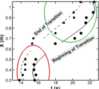
It should be emphasized at the outset that the transition in the ascending phase occurs via laminarization, i.e. initially turbulent boundary layer becomes laminar as the transition front moves downstream in response to the progressively smaller Reynolds number at higher altitude. The experimentally determined transition locations from Table 3 of Ref. [3] are plotted in Fig. 1 for a small time window in the ascending phase that corresponds to approximately 14 to 23 seconds into the flight. The times corresponding to both the boundary between laminar and transitional flow (i.e., time for transition onset) and the boundary between transitional and fully turbulent flow (i.e., “end of transition”) are plotted in the figure. The determination of transition is somewhat subjective, and depends on the criteria and type of sensor used for detection. In these results for ascent, transition end is defined as the time corresponding to a well-defined departure from the turbulent heat transfer, as measured by thermocouples. Transition onset is the time at which heat transfer appears to have fully relaxed to a laminar value.
During the window between 14 and 23 seconds, the transition onset front moves from X = 0.3 m over the first half of cone length to 1.05 m near the end of the cone. The circular and square symbols represent, respectively, the onset and the ending of transition. The lines are curve fits through these data points. The solid line is a curve fit for the onset of transition and the dashed line is a curve fit for the end of transition. Two distinct regions in Figure 1 can be identified: (1) a region of rapid transition front movement (enclosed by the red ellipse), in which transition happens almost simultaneously upstream of X = 0.5 m, and (2) a region of relatively gradual transition front movement (enclosed by the green ellipse). According to Ref. [3], the rapid transition behavior may be attributed to a boundary-layer tripping effect due to the existence of two locations of material discontinuities at approximately X = 0.1 and 0.2 m, respectively. The latter region enclosed by the green ellipse in Figure 1 leaves a window of approximately 5 seconds in which second-mode N-factor correlations with the experiment can be carried out.
Mean flow computations are carried out for different instances of flight from 16 to 23 seconds in intervals of 1 second (and 0.5 seconds, occasionally). The boundary-layer edge Mach number at X = 0.55m (mid-cone) is shown in Fig. 2(a) as a function of time and the ratio of wall temperature to wall adiabatic temperature along the cone are shown in Fig. 2(b) for selected cases. Similar to many hypersonic flight configurations, the surface temperatures downstream of the nose are considerably smaller than the local temperatures corresponding to an adiabatic thermal boundary condition. Thus, no significant first mode instability is expected during the selected window from the ascent phase and this was confirmed by the calculations. The linear instability phase is, therefore, dominated by second mode disturbances. The robustness of findings with respect to uncertainty in surface temperatures was directly confirmed via computations for different temperature distributions.
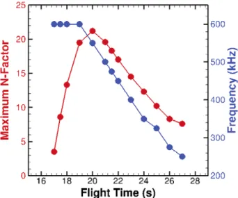
Based on these mean flow computations, N-factors for each instance of flight in this time range are computed. The maximum N-factors and the corresponding frequencies are shown in Fig. 3. It can be seen that the mean flow at t = 20 seconds gives rise to the largest N-factor of N = 21.2 among all instances for which computations were performed. By t = 27 seconds, the N-factor drops to 7.6, indicating a progressively less unstable boundary layer. At the other end of the time window, t = 17 seconds, the maximum N-factor is only 3.5, and yet the experiment shows that there exists large regions of turbulent flow over the cone. This may also be attributed to the tripping effect discussed earlier.
Based on the N-factor computations (Fig. 4) and experimental data (the portion of the fitted curve for the onset of transition that falls within the green ellipse in Figure 1) between 18 and 23 seconds into the flight, the N-factor value correlating with the onset of transition was found to be approximately 13. Quantifiable contributions to the uncertainty in N-factor correlation were also determined. The factors influencing the accuracy of the N-factor correlation include: uncertainties in the surface temperature distribution which must be specified as a boundary condition during mean flow computations; uncertainties in the actual angle of attack during the flight; and uncertainties about the freestream conditions of the flight at each instant of the trajectory. The effect of these uncertainties on the N-factor correlation was found to be small. The uncertainty due to some other factors was difficult to quantify and, hence, was not addressed. One such factor corresponds to the uncertainty in the data reduction process involving the time histories of surface temperature and/or heat flux measured by the thermocouples and heat flux gauges, respectively. It pertains to the noise in the raw measurements and its impact on the estimates of the times for the onset and the end of transition, respectively. Furthermore, determining the times for the onset and the end of transition based on the inferred time histories at a given transducer location also involved some subjectivity as noted in Refs. [3, 6].
The effect of changes in the surface geometry due to steps near material discontinuities was addressed in Ref. [6], wherein the effect of backward facing steps on second mode amplification was computed. It was found that, because the anticipated step locations near the material discontinuities on the model (X = 0.113 m and 0.213 m) were sufficiently farther upstream of the range of amplification for the relevant second mode disturbances, the effect of steps on second mode amplification during the trajectory window of interest was deemed to be secondary. Of course, this does not rule out other mechanisms by which the step excrescences could have influenced transition (e.g., increased receptivity, seeding of streamwise vorticity via azimuthal variations in step height, etc.). Investigation of these mechanisms was deferred to a future study.
III. Re-entry Phase
As described in Refs. [3] and [4], the angle of attack during the re-entry phase of HIFiRE-1 flight departed substantially from the design value of zero degrees. The instrumentation pattern for the HIFiRE-1 model was designed to provide detailed 2D maps of surface temperature and/or heat flux over the majority of the cone surface. However, as a byproduct of the spinning of the (axisymmetric) cone model during flight, information regarding the crossflow transition behavior could have been obtained by using data along the cone meridians with a relatively dense streamwise spacing of surface transducers. The analysis of transition based on the data from thermocouples and heat transfer gauges was complicated by the large temporal variations in the angle of attack as well as the drift in thermocouples prior to transition onset during the reentry phase [3]. However, valuable information was gained from high-frequency pressure measurements, especially those obtained via the pressure transducer PHBW1 at X = 0.85m. The findings from Refs. [3−4] were used to select specific flow conditions for computational analysis as listed in Table I.
Table I. Freestream conditions at selected times during descent phase. Flow Condition Time (s) (deg) α P∞ (Pascal) T∞ (K) M∞ Unit Re (106/m) Altitude (km) R1 481.3 13.60 1126.975 230.508 6.931 2.40 30.611 R2 483.7 9.60 2278.999 223.175 6.974 5.10 25.864 R3 485.0 7.50 3317.379 216.258 7.030 7.80 23.426 R4* 485.0 6.14 3491.140 217.886 7.196 8.32 23.461 * : earlier version of trajectory, angle of attack based on smoothing of raw data
As described in Ref. [5], he higher amplitude, quasi-periodic surface pressure fluctuations were first discernable within the time history of the PHBW1 signal at approximately 481.11 seconds. The frequency of these disturbances (or, effectively, an azimuthal wavenumber based on the cone roll rate) could be visually estimated using the signal window between 481.25 seconds and 481.26 seconds. Accordingly, the trajectory point corresponding to t = 481.3 seconds was selected to ensure that the computed basic flow would support a measurably strong stationary crossflow instability, with due allowance for the effects of the significant uncertainty in the angle of attack α. The data analysis also indicated the first turbulent signal along the windside ray at t = 484.25 seconds. The last identifiable quasi-periodic fluctuations prior to the breakdown to turbulence were observed within the crossflow region at approximately t = 484.58 seconds. At t = 485 seconds (condition R3 from Table I), the flow at X = 0.85m was believed to be turbulent at all azimuthal locations. The flow conditions corresponding to R4 were derived from an earlier version of the flight trajectory and the angle of attack was based on a smoothing of the raw angle of attack estimates based on surface pressure measurements. The differences between cases R3 and R4 illustrate the increased uncertainty in flow conditions during the re-entry phase. The intermediate trajectory point R2 at t = 483.7 seconds was selected for computational analysis for two specific reasons: (i) a Reynolds number value that is approximately halfway between the two extrema corresponding to flow conditions R1 and R3, and (ii) its close proximity to the trajectory point where the periodic pressure fluctuations (normalized by the local pressure) are at a maximum.
The flow configuration R4 also resembles the ground test configuration for quiet tunnel experiments at Purdue University in terms of the cone half-angle and the angle of attack [9], which supports second mode instabilities along the windward and leeward lines and strong crossflow instabilities in between. Even though the model surface temperatures during the ground experiment are comparable to those in the HIFiRE-1 flight experiment, the
freestream static temperature is considerably lower than that in flight. Because of the considerably higher value of the ratio of model surface temperature to adiabatic surface temperature in the ground experiment, that configuration also supports modest amplification of first mode waves [10], which is not anticipated in the flight case.
This paper outlines the computational analysis pertaining to the trajectory point R1 at t = 481.3 seconds, which highlights the effects of a moderately high angle of attack (α/θc = 1.94) on the basic state as well as the flow
instability characteristics. A brief set of results pertaining to stability predictions for the flow condition R4 are also included. The analysis of crossflow instabilities at t = 481.3 seconds and t = 485 seconds should also provide an opportunity for a preliminary comparison between the linear stability based transition correlation for the HIFiRE-1 model with the earlier findings for the Pegasus flight experiment [11]. More comprehensive analysis of the transition behavior during the reentry phase including the flow conditions R2 and R3 is deferred to Ref. [12]. Because of drift issues with a number of surface thermocouples during the exo-atmospheric segment of the trajectory, the surface temperature distributions used for the mean flow computation pertaining to the reentry cases were based entirely upon the thermal analysis using the TOPAZ code. It was assumed that no unsteady vortex shedding occurs at the flow conditions of interest and, therefore, that the (undisturbed) laminar basic state is purely stationary and, furthermore, symmetric with respect to both windward and leeward planes of symmetry.
Fig. 5 presents an overview of the basic state at t = 481.3 seconds in the form of Mach number contours at selected axial locations. The flow contours at the downstream three stations are qualitatively similar. They are suggestive of a separation of the secondary flow near θ = 180±41 degrees, followed by a roll up between the separation location and the leeward plane of symmetry. The presence of crossflow separation over cones at relatively large angles of attack is well-known in the literature and has been confirmed in both experiments [13] and computations based on a parabolic approximation to the Navier-Stokes equations [14]. The roll-up of the secondary flow appears to cause the near pinching of an inverted tear drop shaped structure centered on the leeward meridian. This structure consists of relatively slow moving parcels of fluid that continue to lift away from the surface at increasing X locations, possibly as a result of self-induced velocity. Analogous features have been observed in steady state computations of laminar flow behind an isolated roughness element [15]. The above-mentioned structure is nearly circular at the farthest upstream location, but becomes increasingly oblong over the length of the cone.
The presence of crossflow separation is confirmed by the limiting surface streamlines as shown in Fig. 6(a). These streamlines also confirm the nearly conical behavior of the separated crossflow, except in the vicinity of the nose where the onset of crossflow separation occurs (Fig. 6(b)). A close up view of the surface streamlines near the end of the cone (Fig. 6(c)) provides a hint of a more complex structure underneath the large scale roll-up, perhaps in the form of secondary vortices. The circumferential variations in both the azimuthal shear stress and the total shear stress at selected axial stations are shown in Figs. 7(a) and 7(b), respectively. In addition to confirming the conical behavior of the crossflow separation characteristics, Fig. 7(a) also confirms the existence of an inner region of secondary separation with positive values of azimuthal shear stress.
Despite the finite nose radius (Ren ≈ 6,000), a non-uniform surface temperature distribution, and the presence of
crossflow separation, the axial velocity profiles within the boundary layer along the windward plane of symmetry are nearly similar as seen from Figs. 8(a)-(b). Velocity profiles along the leeward line do not exhibit self-similarity and the heat flux and wall shear distributions do not follow an X-1/2 decay along the symmetry line. Circumferential variation of streamwise, crossflow and wall-normal velocity profiles at X = 0.85 m is shown in Figs. 9(a) through 9(c), respectively. As may be expected, Fig. 9(b) indicates a reversal in the crossflow direction beyond the onset of crossflow separation. The roll-up of the separated secondary flow is correspondingly manifested in a change in the sign of the wall-normal velocity component (Fig. 9(c)).
Given the relatively strong spanwise variations in the vicinity of the leeward meridian, a conventional stability analysis of the velocity profiles along the leeward plane is not meaningful. It is, however, appropriate to perform a stability analysis for the boundary layer flow along the windward plane of symmetry. N-factor curves for axisymmetric second mode disturbances at various frequencies are shown in Fig. 10. The peak N-factor values at X = 0.85 m (the location of the PHBW1 transducer) and over the entire length of the cone are approximately 4.8 and 6.4, respectively. Based on the correlations derived from the ascent phase analysis, transition onset along the windward plane is not expected at t = 481.3 seconds. This finding is consistent with the flight data analysis, which had indicated the onset of transition along the windward line at approximately t = 484.25 seconds.
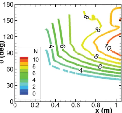
The analysis of crossflow instabilities away from the symmetry planes is considered next. The time history of pressure disturbances measured by the high-frequency transducer PHBW1 is suggestive of the presence of stationary crossflow instability modes with surface pressure disturbance levels of approximately 3.5 percent of the free-stream static pressure [4]. A classical stability analysis was performed for stationary disturbances of fixed azimuthal wavenumber ranging from 20 to 200. The spatial amplification rate is integrated along various trajectories that are aligned with the streamline direction outside the boundary layer. Fig. 11 (a) illustrates the comparison between the inviscid streamline pattern and the limiting surface streamlines presented earlier in Fig. 6. Contours of the peak N-factor value (i.e., maximized over all azimuthal wavenumbers) as a function of location over the cone surface are plotted in Fig. 11(b). It is seen that, for X = 0.85 m, the highest N-factor values are observed within a narrow band of azimuthal locations near θ = 102 degrees relative to the windward meridian. The associated N-factor value is approximately 9. For the Pegasus flight experiment, the onset of crossflow transition was correlated with stationary N-factors (computed using group velocity trajectories) between the range of 7 and 12.4 [11]. However, the comparable N-factor of 9 in the present case is not necessarily inconsistent with the inferred absence of transition in the experiment. That is because boundary layer transition due to stationary crossflow modes is highly sensitive to the external disturbance environment and, particularly, to the surface finish characteristics. Crossflow amplification factors exceeding N=12 have been noted in subsonic flight experiments with smooth surfaces [16].
The range of azimuthal wavenumbers that are most amplified at X = 0.85 m corresponds to n≈ 60−80. Based on Fig. 12 from Ref. [4], one estimates that the quasi-periodic pressure disturbances recorded by the PHBW1 transducer corresponds to an azimuthal wavenumber of n≈ 80 for a cone spinning rate of 4 cycles per second and a wavenumber of approximately n≈ 90 for a spinning rate of 3.5 cycles per second. The observed azimuthal location of θ = 75 degrees is noticeably different from the center of peak N-factor values at X = 0.85 m. This discrepancy could, in part, be caused by the ad hoc approximations required to compute crossflow N-factors in an azimuthally varying boundary layer flow. In particular, we note that the propagation of crossflow disturbances in azimuthally inhomogeneous boundary layers is strongly dependent on a sufficient knowledge of the source of the instability field. Yet, the ad hoc analysis has provided useful information regarding the strength of instability amplification and the frequency-wavelength characteristics of the dominant instability modes.
Instability amplification characteristics for the case R4 are examined next. Due to the lower angle of attack, the crossflow behavior in this case is significantly different from that in case R1 as shown by the Mach number contours in Fig. 12(a). The N-factors along the windward line reach 14 just past the midway point of the cone and approach 23 near the end of the cone. The N-factors along the leeward line are considerably smaller, only about 9.5. This weaker second mode instability along the leeward plane is attributed to the substantially modified local mean flow as a result of the convergence of secondary flow from either side of this plane [17]. Because of the finite angle of attack, crossflow instability is, again, important away from the windward and leeward planes. Figure 12(b) shows the N-factor contours for stationary crossflow instability, obtained as an envelope of the amplification curves for stationary modes of fixed azimuthal wavenumber. The N-factor reaches a value of 14 just before X = 0.5 m. The N-factor values shown in Fig. 12 are capped off at 14 to emphasize that crossflow transition is likely to occur over the middle portion of the cone, but the actual N-factors reach a maximum of approximately 26 at the end of the cone. The large N-factors for the R4 case are consistent with the finding from the flight measurements that the flow over the aft portion of the cone is turbulent by t = 485 seconds.
III. Conclusions
The HIFiRE-1 flight experiment by AFRL has provided a valuable and, in many ways, a unique database for boundary layer transition over a circular cone model at varying Mach number, Reynolds number, and angle of attack. Based on measurements over a relevant subset of the ascent trajectory, the onset of transition due to second mode instabilities is found to correlate with an N-factor of approximately 13. Transition at early times and lower Mach numbers is believed to be influenced by step excrescences on the model. Due to the higher angle of attack during the descending phase, instability characteristics along the leeward line of symmetry are altered substantially and strong crossflow instability exists in between the windward and leeward planes of symmetry. Linear stability correlations for strongly inhomogeneous 3D boundary layers involve ad hoc assumptions that must be substantiated via case by case comparisons with numerical simulations and/or experimental measurements. Preliminary findings presented herein confirm the presence of a moderate instability at t = 481.3 seconds. The locations of peak N-factor values and corresponding azimuthal wavenumbers are approximately consistent with the findings based on the
analysis of the flight measurements [4]. This finding lends credence to the belief that the higher amplitude, quasi-periodic fluctuations measured by the high frequency transducers are likely to be associated with stationary crossflow instability.
The substantial uncertainty in angle of attack during the reentry phase limits the extent of comparison between flight data and computational predictions. Future computations will address the sensitivity of the computed results to the angle of attack as well as direct numerical simulations pertaining to the effect of crossflow separation on the propagation of both crossflow and second mode instabilities.
Acknowledgments
The work of NASA authors was performed as part of the Aerodynamics, Aerothermodynamics, and Plasma Dynamics (AAP) element of the Hypersonics Project of NASA’s Fundamental Aeronautics Program (FAP).
References
1. Kimmel, R. L., Adamczak, D., Gaitonde, D., Rougeux, A., and Haynes, J. R., “HIFiRE-1 Boundary Layer Transition Experiment
Design,” AIAA Paper 2007-534, 2007.
2. Kimmel, R. L., “Aerothermal Design for HIFiRE-1 Flight Vehicle,” AIAA Paper 2008-4034, 2008.
3. Kimmel, R. L., Adamczak, D., and DSTO AVD Brisbane Team, “HIFiRE Preliminary Aerothermodynamic Measurements,”
AIAA Paper 2011-3413, 2011.
4. Adamczak, D., Kimmel, R. L., and DSTO AVD Brisbane Team, “HIFiRE-1 Trajectory Estimation and Preliminary Experimental
Results,” AIAA paper 2011-2358, 2011.
5. Stanfield, S., Kimmel, R. L., and Adamczak, D., “HIFiRE-1 Flight Data Analysis: Boundary Layer Transition
Experiment During Reentry,” AIAA Paper 2012-1087, 2012.
6. Li, F., Choudhari, M., Chang, C.-L., Kimmel, R., Adamczak, D., and Smith, M., “Transition Analysis for the HIFiRE-1 Flight
Experiment,” AIAA Paper 2011-3414, 2011.
7. http://vulcan-cfd.larc.nasa.gov (Aug. 18, 2011)
8. Chang, C.-L., “LASTRAC.3d: Transition Prediction in 3D Boundary Layers,” AIAA Paper 2004-2542, 2004.
9. Wheaton, B. M., Juliano, T. J., Berridge, D. C., Chou, A., Gilbert, P. L., Casper, K. M., Sheen, L. E., and Schneider, S. P.,
“Instability and Transition Measurements in the Mach-6 Quiet Tunnel,” AIAA Paper 2009-3559,2009.
10. Li, F., Choudhari, M., Chang, C.-L., and White, J., “Analysis of Instabilities in Non-Axisymmetric Hypersonic Boundary Layers
over Cones,” AIAA Paper 2010-4643, 2010.
11. Malik, M., Li, F., and Choudhari, M., “Analysis of Crossflow Transition Flight Experiment aboard Pegasus Launch Vehicle,”
AIAA Paper 2007-4487, 2007.
12. Li, F., Choudhari, M., Chang, C.-L., White, J.A., Kimmel, R., Adamczak, D., Borg, M., Stanfield, S., and Smith, M., “Stability
Analysis for HIFiRE Experiments,” To be presented at the AIAA 42nd Fluid Dynamics Conference, New Orleans, LA, June
25-28, 2012.
13. Tracy, R.R., “Hypersonic Flow Over a Yawed Circular Cone,” California Institute of Technology, Aeronautical Lab., Memo 69,
1963.
14. Lin, T.C. and Rubin, S.G., “Viscous Flow Over a Cone at Moderate Incidence. II: Supersonic Boundary Layer,” J. Fluid Mech.,
Vol. 59, March 1973, pp. 593-620.
15. Choudhari, M., Li, F., Wu, M., Chang, C.-L., and Edwards, J.A., “Laminar Turbulent Transition behind Discrete Roughness
Elements in a High-Speed Boundary-Layer,” AIAA Paper 2010-1575, 2010.
16. Carpenter, A.L., Saric, W.S., and Reed, H.L., “Laminar Flow Control on a Swept Wing with Distributed Roughness,” AIAA
Paper 2008-7335, 2008.
17. Choudhari, M., Chang, C.-L., Jentink, T., Li, F., Berger, K., Candler, G., and Kimmel, R., “Transition Analysis for the HIFiRE-5
Vehicle,” AIAA Paper 2009–4056, 2009.
Figure 1. Transition front. Circular and square symbols represent, respectively, experimentally measured onset and ending of transition as given in Ref. [3]. Lines represent curve fit through experimental data. Solid line is a curve fit through transition onset data and the dashed line is acurve fit through the end-of-transition data. Red ellipse encloses region of rapid movement in transition front and green ellipse encloses region of slower transition front movement.
(a) Boundary-layer edge Mach number (b) Temperature ratio
Figure 2. Boundary-layer edge Mach number at X = 0.55m and ratio of wall temperature to wall adiabatic temperature during selected time interval from the ascent phase.
Figure 3. Temporal variation of maximum N-factor over the length of the cone (red line and symbols) and the corresponding second mode frequency (blue line and symbols) during the trajectory segment of interest during ascent.
t (s) Me at X = 0.55 m 16 18 20 22 24 26 28 30 3 3.5 4 4.5 5 5.5 X (m) Tw /T ad b 0.2 0.4 0.6 0.8 1 0.2 0.3 0.4 0.5 0.6 0.7 t = 16 s t = 18 s t = 20 t = 26 s t = 21.5 s t = 24 s t = 30 s
(a) t = 18 s (b) t = 19 s
(c) t = 20 s (d) t = 21 s
(e) t = 22 s (f) t = 23 s
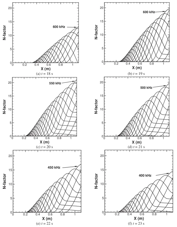
Figure 4. N-factor evolution for second mode disturbances of various frequencies from t = 18 to 23 seconds. The disturbance frequency decreases by 25 kHz across each adjacent pair of N-factor curves.
X (m) N-fact o r 0 0.2 0.4 0.6 0.8 1 0 5 10 15 20 600 kHz X (m) N -fa c to r 0 0.2 0.4 0.6 0.8 1 0 5 10 15 20 600 kHz , X (m) N-fact o r 0 0.2 0.4 0.6 0.8 1 0 5 10 15 20 550 kHz , X (m) N -fa c to r 0 0.2 0.4 0.6 0.8 1 0 5 10 15 20 500 kHz X (m) N-fa c to r 0 0.2 0.4 0.6 0.8 1 0 5 10 15 20 450 kHz X (m) N-fa c to r 0 0.2 0.4 0.6 0.8 1 0 5 10 15 20 400 kHz
Figure 5. Mach number contours at selected axial locations for case R1
(a) Overall (b) Close-up view near nose (c) Close-up view near end of cone Figure 6. Limiting surface streamlines for case R1 (t = 481.3 seconds). Top boundary of each image corresponds
to leeward line.
(a) Azimuthal shear stress (b) Total shear stress
(a) 0.4 m < X < 0.6 m. (b) X > 0.6m. Figure 8. Axial velocity profiles at various stations along windward meridian.
(a) Streamwise velocity (b) Crossflow velocity (c) Wall-normal velocity Figure 9. Velocity profiles at X = 0.85 m.
Fig. 11(a). Inviscid streamline pattern (red curves) used for N-factor calculation along with limiting surface streamlines (black curves).
Fig. 11(b). N-factor contours for stationary crossflow mode disturbances. Bottom of the figure corresponds to windward side and the top boundary is leeward side. Figure 11. Analysis of stationary crossflow instability for trajectory point R1 at t = 481.3 seconds
Fig. 12(a). Mach number contours at selected axial locations.
Fig. 12(b). N-factor contours for stationary crossflow mode disturbances. Bottom of the cone is windward side and top is leeward side.