Open Access Theses Theses and Dissertations
Fall 2014
Crossflow Transition At Mach 6 On A Cone At
Low Angles Of Attack
Ryan O. Henderson
Purdue UniversityFollow this and additional works at:https://docs.lib.purdue.edu/open_access_theses Part of theAerospace Engineering Commons
This document has been made available through Purdue e-Pubs, a service of the Purdue University Libraries. Please contact [email protected] for additional information.
Recommended Citation
Henderson, Ryan O., "Crossflow Transition At Mach 6 On A Cone At Low Angles Of Attack" (2014).Open Access Theses. 334.
ATTACK
A Thesis
Submitted to the Faculty of
Purdue University by
Ryan O. Henderson
In Partial Fulfillment of the Requirements for the Degree
of
Master of Science in Aeronautics and Astronautics
December 2014 Purdue University West Lafayette, Indiana
ACKNOWLEDGMENTS
First and foremost, I would like to thank my advisor, Professor Steven Schneider, for his guidance throughout this research as well as giving me the opportunity to investigate the unknown. I would also like to acknowledge Dr. John Sullivan and Dr. Patrick Rodi, for joining my advisory board. I would also like to acknowledge Lockheed Martin for funding the research.
I would like to acknowledge Robin Snodgrass, Jim Younts, and Jerry Hahn in the ASL machine shop for keeping the tunnel and the experiments operating smoothly. The machine shop humor was also appreciated. John Phillips was also very helpful with all electronic problems I came across.
Though my lab mates taught me much about fluid mechanics, they moreover provided continuous entertainment throughout my time at Purdue. Thanks to Dennis Berridge, Amanda Chou, Brandon Chynoweth, Roger Greenwood, Greg McKiernan, George Moraru, and Chris Ward for the wonderful memories around the lab. Alumni Matt Borg was very helpful with sharing his knowledge of traveling waves. Also thanks to John Schooner and his friend Sam Ball for brightening everyone’s day throughout the semesters.
I would like to specially thank my family for encouragement throughout my grad-uate career, even though most of them don’t know what I do (I work in a tube that blows air). They still believed in me and sent their love whenever I needed it. Most importantly I am indebted to Nicole Quindara for loving and supporting me while suffering through my long hours away and other tunnel nonsense.
TABLE OF CONTENTS
Page
LIST OF TABLES . . . vi
LIST OF FIGURES . . . vii
SYMBOLS . . . xvii ABBREVIATIONS . . . xix ABSTRACT . . . xx 1 INTRODUCTION . . . 1 1.1 Objectives . . . 4 2 BACKGROUND . . . 5 2.1 Crossflow Instability . . . 5 2.1.1 Stationary Mode . . . 7 2.1.2 Traveling Mode . . . 7
2.2 Secondary Instability of Crossflow Vortices . . . 8
2.3 High-Speed Second-mode Instability. . . 8
2.4 Low-Speed Experiments . . . 9
2.5 High-Speed Experiments . . . 11
3 FACILITY . . . 15
3.1 Boeing/AFOSR Mach-6 Quiet Tunnel. . . 15
3.2 Reynolds Number Calculation . . . 18
4 MODELS . . . 20
4.1 Cone Models . . . 20
4.2 Nosetip Radii . . . 24
4.3 Model Positioning . . . 25
4.4 Roughness Elements . . . 25
5 INSTRUMENTATION AND ANALYSIS METHODS . . . 26
5.1 Oscilloscopes . . . 26
5.2 Hot Films . . . 26
5.3 Pressure Measurements . . . 27
5.3.1 Kulite Pressure Transducers . . . 27
5.3.2 PCB Pressure Transducers . . . 28
5.3.3 Power Spectra . . . 28
Page
5.4.1 Thermocouples . . . 30
5.4.2 Temperature Sensitive Paint . . . 31
5.5 Roughness Measurements . . . 41
6 RESULTS AT ZERO ANGLE OF ATTACK . . . 42
6.1 Tunnel Noise Effects . . . 42
6.2 Reynolds Number Comparison . . . 46
6.3 0◦ AoA Symmetry . . . 49
6.4 Second-mode Amplitudes . . . 50
6.5 Pate’s Correlation . . . 52
7 STATIONARY CROSSFLOW INSTABILITY . . . 54
7.1 Defining Stationary Crossflow Vortices . . . 54
7.2 Reynolds Number Comparison . . . 54
7.2.1 90◦ Ray Results . . . 54
7.2.2 120◦ Ray Results . . . 58
7.3 Angle of Attack Comparison . . . 62
7.3.1 Smooth Surface Results . . . 62
7.3.2 Torlon-insert Roughness Results . . . 65
7.4 Stationary Waves under Noisy Flow . . . 70
7.5 Repeatability between Entries . . . 70
8 TRAVELING CROSSFLOW INSTABILITY . . . 75
8.1 Wave Properties. . . 75
8.1.1 Coherence . . . 78
8.1.2 Wave Angle . . . 79
8.1.3 Phase Speed . . . 80
8.1.4 Instability Analysis . . . 81
8.2 Reynolds Number Comparison . . . 82
8.3 Angle of Attack Comparison . . . 85
8.4 Tunnel Noise Comparison . . . 89
8.5 Similarity between Pressure Sensors . . . 92
9 INTERACTIONS BETWEEN STATIONARY & TRAVELING WAVES 96 9.1 Entry 4 Interactions . . . 96
9.1.1 E4 Roughness Application and Measurement . . . 97
9.1.2 E4 Roughness Effects . . . 100
9.2 Entry 6 Interactions . . . 107
9.2.1 E6 Roughness Application and Measurement . . . 107
9.2.2 E6 Roughness Effects . . . 110
9.3 Interaction Analysis. . . 118
10 POSSIBLE SECONDARY INSTABILITY OF THE STATIONARY CROSS-FLOW VORTICES . . . 121
Page
10.1.1 Disturbances near the 60◦ and 95◦ rays at 4◦ AoA . . . 121
10.1.2 Disturbances near the 120◦ ray at 4◦ AoA . . . 125
10.1.3 Disturbances near the 139.5◦, 150◦, and 165◦ ray at 3◦ AoA 128 10.2 Runs with Vortices over Pressure Sensors without High-Frequency Dis-turbances . . . 135
10.3 Disturbance Analysis . . . 138
11 CONCLUSIONS AND FUTURE WORK . . . 141
11.1 Conclusions . . . 141 11.2 Future Work . . . 142 LIST OF REFERENCES . . . 144 APPENDICES A Symmetry Check . . . 149 B Roughness Measurements. . . 150
C Tunnel Conditions for All Runs . . . 151
LIST OF TABLES
Table Page
4.1 Crossflow Cone sensor locations. . . 21
4.2 Ward Cone sensor locations. Positive degrees from sensor ray are towards the upward direction in reference to Figure 4.2. . . 22
4.3 Ward Cone Kulite Array sensor locations. Positive degrees from sensor ray are towards the upward direction in reference to Figure 4.2. . . 23
8.1 Traveling wave characteristics for frequencies from 30 to 50 kHz. All runs shown are at 4◦ AoA. . . 82
9.1 Smooth and added roughness effects on traveling-wave amplitude. PSDs integrated from 20 to 80 kHz. All runs at Re= 3.62±0.04×10⁶/ft. . . 119
9.2 Matching smooth and added-roughness runs to compare traveling-wave amplitudes. . . 120
10.1 Disturbance properties for all tests with possible secondary instabilities. All sensors at x = 14.3-in. Asterisk denotes Kulite sensors where the frequency response past 60 kHz is not known. . . 140
A.1 Percent difference of second-mode amplitudes against the mean amplitude computed at 0◦ AoA.Re= 3.65×10⁶/ft. All data from PCB sensors. . 149
B.1 Roughness measurements of cone surface and discrete roughness elements. 150 C.1 Run Schedule for Entry 1. . . 152
C.2 Run Schedule for Entry 2. . . 153
C.3 Run Schedule for Entry 2 continued. . . 154
C.4 Run Schedule for Entry 3. . . 155
C.5 Run Schedule for Entry 4. . . 156
C.6 Run Schedule for Entry 4 continued. . . 157
C.7 Run Schedule for Entry 5. . . 158
C.8 Run Schedule for Entry 5 continued. . . 159
C.9 Run Schedule for Entry 6. . . 160
LIST OF FIGURES
Figure Page
1.1 Mechanisms of boundary-layer transition. Redrawn from Fig. 1 of
Refer-ence [4]. . . 2
1.2 Shawdowgraph of noise effects of turbulent spots on a sharp cone at Mach 4.31. Image courtesy of Dan Reda. . . 3
2.1 Boundary layer, crossflow, and resultant velocity profiles. Image from Adams [10]. . . 5
2.2 Boundary layer streamlines on a 7◦ half-angle cone at 6◦ angle of attack. With permission from author [12]. . . 6
2.3 Path of acoustic mode and property profiles in the boundary layer, where U(y) is the velocity profile, and p(y) is the pressure disturbance profile. Redrawn from Fig. 2 in reference [24]. . . 9
2.4 Traveling crossflow contour plots at 3◦ angle of attack. Fig. 14c from reference [41]. . . 13
3.1 Schematic of the Boeing/AFOSR Mach-6 Quiet Tunnel. . . 15
3.2 Schematic of BAM6QT with 7.5◦ cone model. Dimensions are in inches [meters]. . . 17
3.3 Porthole optical access with typical cone model. . . 17
4.1 Crossflow Cone with TSP coating. . . 20
4.2 Ward Cone schematic. . . 22
4.3 Crossflow Cone nosetip. . . 24
4.4 Ward Cone nosetip. . . 24
5.1 Sketch of TSP apparatus. . . 34
5.2 Typical CCD camera and LED array placement. . . 35
5.3 Typical TSP calibration using a SB gauge. E6R6, 4◦ AoA, quiet flow, Torlon insert, SB gauge atx= 10.9-in. on the 120◦ray. Re= 3.68×10⁶/ft, Po = 156.8 psia,To = 299.2◦F, Tw = 93.4◦F. . . 37
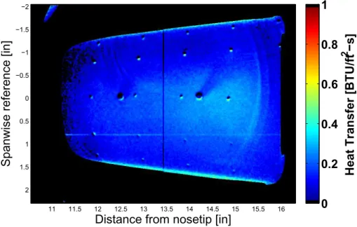
5.4 Heat transfer contour of E3R2. 0◦ AoA, quiet flow, smooth surface. Re= 3.25×10⁶/ft, P o = 137.6 psia, To = 295.5◦F, Tw = 79.5◦F. . . 38
Figure Page
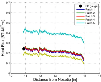
5.5 Axial heat flux profiles of E3R2 for calibrations from each patch.
The-oretical heat transfer and SB gauge readout at time of process are also
shown. . . 39
5.6 Heat transfer contour of E4R1. 4◦ AoA, quiet flow, smooth surface. Re=
3.65×10⁶/ft, P
o = 156.8 psia, To = 301.7◦F, Tw = 74.6◦F. . . 40
5.7 Axial heat flux profiles of E4R1 for calibrations from each patch, SB gauge
readout at time of process. . . 40
6.1 PSD of quiet results (solid) for E1R2 Re = 2.79×10⁶/ft, Noisy results
(dotted) E1R3 Re= 2.89×10⁶/ft, all traces from PCB sensors. . . . . . 43
6.2 Heat transfer contour of E1R2 0◦AoA, quiet flow, smooth surface. Re =
2.79×10⁶/ft, Po = 114.9 psia, To = 283.5◦F, Tw = 77.3◦F. . . 44
6.3 Heat transfer contour of E1R3 0◦AoA, noisy flow, smooth surface. Re =
2.89×10⁶/ft, Po = 113.4 psia, To = 293.9◦F, Tw = 83.3◦F. . . 44
6.4 PSD of quiet results (solid) for E1R5 Re = 3.21×10⁶/ft, Noisy results
(dotted) E1R6 Re= 3.28×10⁶/ft, all traces from PCB sensors. . . . . . 45
6.5 PSD of quiet results (solid) for E1R7 Re = 3.67×10⁶/ft, Noisy results
(dotted) E1R8 Re= 3.57×10⁶/ft, all traces from PCB sensors. . . . . . 46
6.6 PSD of noisy spectra for runs E1R3 (blue), E1R6 (green), and E1R8 (red),
all traces from PCB sensor at x= 9.2-in. . . 47
6.7 PSD of noisy spectra for runs E1R3 (blue), E1R6 (green), and E1R8 (red),
all traces from PCB sensor at x= 10.9-in. . . 48
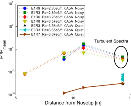
6.8 PSD of quiet spectra for runs E1R2 (blue), E1R5 (green), and E1R7 (red),
all traces from PCB sensor at x= 14.3-in. . . 48
6.9 PSD of quiet spectra for run E3R3, all traces from PCB sensors at x =
14.3-in. using the Ward Cone. . . 50
6.10 Second-mode amplitudes as a function of distance from nosetip. . . 51
6.11 Second-mode amplitudes as a function of Reynolds number with
charac-teristic length x. . . 51
6.12 Comparison of Pate’s Correlation with experimental results from E1R3,
E1R6, and E1R8. Uncertainty bar edges at pressure sensor positions. . 53
7.1 Heat transfer contour of E4R3. 4◦AoA, quiet flow, smooth surface, Kulites
near the 90◦ ray. Re= 2.81×10⁶/ft, Po = 118.8 psia, To = 295.7◦F, Tw =
Figure Page
7.2 Heat transfer contour of E4R2. 4◦AoA, quiet flow, smooth surface, Kulites
near the 90◦ ray. Re= 3.29×10⁶/ft, Po = 139.9 psia, To = 297.7◦F, Tw =
82.3◦F. . . 56
7.3 Heat transfer contour of E4R1. 4◦AoA, quiet flow, smooth surface, Kulites
near the 90◦ ray. Re= 3.66×10⁶/ft, Po = 156.8 psia, To = 301.7◦F, Tw =
74.6◦F. . . 56
7.4 Spanwise heat transfer profile of E4R3, E4R2, and E4R1 at x = 12.1-in,
4◦AoA, quiet flow, smooth surface. . . 57
7.5 Spanwise heat transfer profile of E4R3, E4R2, and E4R1 at x = 13.0-in,
4◦AoA, quiet flow, smooth surface. . . 57
7.6 PSD of E4R3, E4R2, and E4R1. 4◦AoA, Quiet flow, smooth surface, PCB
sensor at the 150◦ ray. . . 58
7.7 Heat transfer contour of E5R5. 4◦AoA, quiet flow, smooth surface, Kulites
near the 120◦ ray. Re= 3.26×10⁶/ft,Po = 140.0 psia,To = 302.3◦F,Tw =
90.3◦F. . . 59
7.8 Heat transfer contour of E5R6. 4◦AoA, quiet flow, smooth surface, Kulites
near the 120◦ ray. Re= 3.71×10⁶/ft,Po = 158.0 psia,To = 299.4◦F,Tw =
95.8◦F. . . 60
7.9 Spanwise heat transfer profile of E5R5 and E5R6 at x = 12.0-in, 4◦AoA,
quiet flow, smooth surface. . . 61
7.10 Spanwise heat transfer profile of E5R5 and E5R6 at x = 13.0-in, 4◦AoA,
quiet flow, smooth surface. . . 61
7.11 Heat transfer contour of E6R12. 2◦AoA, quiet flow, smooth surface,
Kulites near the 90◦ray. Re= 3.64×10⁶/ft,P
o = 155.7 psia,To = 304.9◦F,
Tw = 79.8◦F. . . 62
7.12 Heat transfer contour of E6R31. 3◦AoA, quiet flow, smooth surface,
Kulites near the 90◦ray. Re= 3.58×10⁶/ft,Po = 157.2 psia,To = 313.1◦F,
Tw = 86.7◦F. . . 63
7.13 Heat transfer contour of E5R1. 4◦AoA, quiet flow, smooth surface, Kulites
near the 90◦ ray. Re= 3.69×10⁶/ft, Po = 157.6 psia, To = 300.3◦F, Tw =
90.4◦F. . . 64
7.14 Spanwise heat transfer profile of E6R12, E6R31, and E5R1 atx= 13.5-in,
Figure Page
7.15 Heat transfer contour of E6R17. 2◦AoA, quiet flow, Torlon insert, Kulites
near the 120◦ ray. Re= 3.60×10⁶/ft,P
o = 156.8 psia,To = 309.3◦F,Tw =
79.8◦F. . . 66
7.16 Heat transfer contour of E6R39. 3◦AoA, quiet flow, Torlon insert, Kulites
near the 120◦ ray. Re= 3.61×10⁶/ft,P
o = 157.0 psia,To = 308.1◦F,Tw =
86.7◦F. . . 66
7.17 Heat transfer contour of E6R4. 4◦AoA, quiet flow, Torlon insert, Kulites
near the 120◦ ray. Re= 3.62×10⁶/ft,Po = 156.8 psia,To = 306.2◦F,Tw =
90.4◦F. . . 67
7.18 Spanwise heat transfer profile of E6R12, E6R31, and E5R1 atx= 11.5-in,
quiet flow, Torlon insert. . . 67
7.19 Spanwise heat transfer profile of E6R12, E6R31, and E5R1 atx= 13.5-in,
quiet flow, Torlon insert. . . 68
7.20 Heat transfer contour of E6R4 with vortex labels, quiet flow, Torlon insert. 69
7.21 Axial heat transfer profiles of vortices for E6R4, quiet flow, Torlon insert. 69
7.22 Spanwise profiles along Vortex 2. . . 70
7.23 Heat transfer contour of E3R7. 4◦AoA, noisy flow, smooth surface, Kulites
near the 90◦ ray. Re= 2.89×10⁶/ft, Po = 114.7 psia, To = 301.2◦F, Tw =
83.4◦F. . . 71
7.24 Heat transfer contour of E2R22. 4◦AoA, quiet flow, smooth surface, PCBs
at the 120◦ ray. Re= 3.64×10⁶/ft, P
o = 158.2 psia, To = 308.3◦F, Tw =
85.1◦F. . . 72
7.25 Heat transfer contour of E3R16. 4◦AoA, quiet flow, smooth surface,
Kulites near the 120◦ ray. Re = 3.63×10⁶/ft, P
o = 156.1 psia, To =
302.6◦F, Tw = 94.6◦F. . . 73
7.26 Heat transfer contour of E4R1. 4◦AoA, quiet flow, smooth surface, Kulites
near the 90◦ ray. Re= 3.65×10⁶/ft, P
o = 156.8 psia, To = 301.7◦F, Tw =
74.6◦F. . . 73
7.27 Heat transfer contour of E5R6. 4◦AoA, quiet flow, smooth surface, Kulites
near the 120◦ ray. Re= 3.71×10⁶/ft,P
o = 158.0 psia,To = 299.4◦F,Tw =
90.4◦F. . . 74
7.28 Spanwise heat transfer profile of entries 2, 3, 4, and 5 atx= 13.5-in, quiet
flow, smooth surface. . . 74
8.1 Orientation of coordinate systems for cross-spectral analysis. Drawing
Figure Page
8.2 Schematic of Kulite Array 2 and reference frame used to determine wave
orientation. . . 77
8.3 PSD of E3R4. Quiet flow, smooth surface, Kulites k1, k2, and k3 near the 90◦ ray. . . 78
8.4 Coherence between Kulite sensors for E3R4. . . 79
8.5 Calculated wave angle as a function of frequency for E3R4. . . 80
8.6 Calculated phase velocity as a function of frequency for E3R4. . . 81
8.7 PSD of Reynolds number comparison for traveling-wave frequencies. 4◦AoA, quiet flow, smooth surface, Kulite at the 94.5◦ ray. . . 83
8.8 PSD of Reynolds number comparison for traveling-wave frequencies. 4◦AoA, quiet flow, smooth surface, Kulite at the 124.5◦ ray. . . 84
8.9 RMS fluctuations as a function of the Reynolds number for various az-imuthal rays. RMS in the 20-80 kHz band of power spectra. 4◦ AoA, smooth surface. . . 85
8.10 PSD of angle of attack comparison for traveling wave frequencies. Quiet flow, Torlon insert, Kulite at the 90◦ ray. . . 86
8.11 PSD of angle of attack comparison for traveling wave frequencies. Quiet flow, Torlon insert, Kulite at the 120◦ ray. . . 86
8.12 PSD of angle of attack comparison for traveling wave frequencies. Quiet flow, Torlon insert, PCB sensor at the 150◦ ray. . . 87
8.13 RMS fluctuations as a function of the Reynolds number at the 60◦ ray from windward for 2◦, 3◦, and 4◦ AoA. RMS in the 20-80 kHz band of power spectra. All data taken from entry 6 with Torlon insert installed. 88 8.14 RMS fluctuations as a function of the Reynolds number at the 90◦ ray from windward for 2◦, 3◦, and 4◦ AoA. RMS in the 20-80 kHz band of power spectra. . . 89
8.15 RMS fluctuations as a function of the Reynolds number at the 120◦ ray from windward for 2◦, 3◦, and 4◦ AoA. RMS in the 20-80 kHz band of power spectra. . . 90
8.16 PSD for tunnel noise comparison for traveling-wave frequencies. 4◦ AoA, smooth surface, Kulite at the 90◦ ray. . . 90
8.17 PSD for tunnel noise comparison for traveling wave frequencies. 4◦ AoA, smooth surface, Each sensor type at the 90◦ ray. . . 91
Figure Page 8.18 Wave calculations for E4R9. (a) PSD (b) Coherence (c) Wave angle (d)
Phase velocity . . . 92
8.19 PSD of PCB and Kulite sensors with similar tunnel conditions and sensor
location. 2◦ AoA, quiet flow, Torlon insert, both sensor types at the
90◦ ray. . . 93
8.20 PSD of PCB and Kulite sensors with similar tunnel conditions and sensor
location. 2◦ AoA, quiet flow, Torlon insert, both sensor types at the
120◦ ray. . . 94
8.21 PSD of PCB and Kulite sensors with similar tunnel conditions and sensor
location. 3◦ AoA, quiet flow, Torlon insert, both sensor types at the
90◦ ray. . . 95
8.22 PSD of PCB and Kulite sensors with similar tunnel conditions and sensor
location. 3◦ AoA, quiet flow, Torlon insert, both sensor types at the
120◦ ray. . . 95
9.1 Photographs of Ward Cone during entry 4 testing with initial nail-polish
roughness strip (a) and roughness ring (b). . . 98
9.2 Surface and negative height profile of E4 roughness ring (a) 90◦ and (b)
270◦ from Kulite 3. Profiles from right to left were measured in the
direc-tion of flow. . . 99
9.3 Heat transfer contour of E4R1. 4◦AoA, quiet flow, smooth surface, Kulites
near the 90◦ ray. Re= 3.66×10⁶/ft, Po = 156.8 psia, To = 301.7◦F, Tw =
74.6◦F. . . 100
9.4 Heat transfer contour of E4R23. 4◦AoA, quiet flow, E4 roughness strip,
Kulites near the 90◦ray. Re= 3.68×10⁶/ft,Po = 157.2 psia,To = 299.6◦F,
Tw = 79.9◦F. . . 101
9.5 Heat transfer contour of E4R29. 4◦AoA, quiet flow, E4 roughness ring,
Kulites near the 90◦ray. Re= 3.66×10⁶/ft,P
o = 157.1 psia,To = 302.1◦F,
Tw = 76.8◦F. . . 101
9.6 Spanwise heat transfer profile of E4R1, E4R23, and E4R29 atx= 12.5-in.
4◦AoA, quiet flow, Kulite array near the 90◦ ray.. . . 102
9.7 Spanwise heat transfer profile of E4R1, E4R23, and E4R29 atx= 13.5-in.
4◦AoA, quiet flow, Kulite array near the 90◦ ray.. . . 103
9.8 Spanwise heat transfer profile of E4R1, E4R23, and E4R29 atx= 14.5-in.
4◦AoA, quiet flow, Kulite array near the 90◦ ray.. . . 103
Figure Page 9.10 PSD of E4R1 (smooth surface), E4R24 (E4 roughness strip), and E4R29
(E4 roughness ring) at x = 14.4-in, 4◦AoA, quiet flow, Kulite 4 at the
87.75◦ ray. . . 105
9.11 PSD of E4R1 (smooth surface), E4R24 (E4 roughness strip), and E4R29
(E4 roughness ring) at x = 14.2-in, 4◦AoA, quiet flow, Kulite 2 at the
92.25◦ ray. . . 106
9.12 Schematic of the stationary and traveling crossflow wave directions. . . 106
9.13 Photograph of Torlon insert assembled to the Ward Cone and nosetip. 108
9.14 Contour of Torlon insert. . . 108
9.15 Profile of Torlon insert using the Keyence digital microscope. Measured
depths of 4.74 mil (120.28 µm) and 5.14 mil (130.44 µm). . . 109
9.16 Profile of Torlon insert using the SJ-130 profilometer. . . 109
9.17 Heat transfer contour of E6R12. 2◦AoA, quiet flow, smooth surface, Kulite
array on the 90◦ ray. Re = 3.64x10⁶/f t, P
o = 155.7 psia, To = 300.4◦F,
Tw = 79.8◦F. . . 110
9.18 Heat transfer contour of E6R15. 2◦AoA, quiet flow, Torlon insert, Kulite
array on the 90◦ ray. Re = 3.63x10⁶/f t, P
o = 156.9 psia, To = 304.9◦F,
Tw = 86.5◦F. . . 111
9.19 Spanwise heat transfer profile of E6R12 and E6R15 atx= 14.0-in. 2◦AoA,
quiet flow, Kulite array near the 90◦ ray. . . 112
9.20 PSD of E6R12 (smooth surface) and E6R15 (Torlon insert) for cone at
2◦AoA under quiet flow. Kulite at 90◦ ray and x= 14.3-in. . . 112
9.21 PSD of E6R12 E6R13 (smooth surface, solid lines) and E6R14 E6R15
(Torlon insert, dotted lines) for cone at 2◦AoA under quiet flow. PCB at
the 120◦ ray andx= 14.3-in. . . 113
9.22 Heat transfer profile of E6R33. 3◦AoA, quiet flow, smooth surface, Kulite
array near the 90◦ ray. Re= 3.63x10⁶/f t, P
o = 153.0 psia, To = 294.5◦F,
Tw = 95.7◦F. . . 114
9.23 Heat transfer profile of E6R34. 3◦AoA, quiet flow, Torlon insert, Kulite
array near the 90◦ ray. Re= 3.63x10⁶/f t, Po = 158.5 psia, To = 310.2◦F,
Tw = 82.4◦F. . . 114
9.24 Spanwise heat transfer profile of E6R33 (smooth surface) and E6R34
Figure Page 9.25 PSD of E6R33 (smooth surface) and E6R34 (torlon insert) for cone at
3◦AoA under quiet flow. Kulite at 90◦ ray and x= 14.3-in. . . 115
9.26 PSD of E6R33 (smooth surface) and E6R34 (torlon insert) for cone at
3◦AoA under quiet flow. PCB at 120◦ ray and x= 14.3-in. . . 116
9.27 Temperature difference contour of E5R1. 4◦AoA, quiet flow, smooth
sur-face, Kulite array near the 90◦ ray. Re = 3.69x10⁶/f t, Po = 157.6 psia,
To = 300.3◦F, Tw = 90.4◦F. . . 117
9.28 Temperature difference contour of E6R1. 4◦AoA, quiet flow, Torlon insert,
Kulite array near the 90◦ ray. Re = 3.70x10⁶/f t, P
o = 150.4 psia, To =
277.8◦F, Tw = 77.5◦F. . . 117
9.29 PSD of E5R27 (smooth surface) and E6R3 (Torlon insert) for cone at
4◦AoA under quiet flow. Kulite at 94.5◦ ray andx= 14.3-in. . . 118
10.1 Heat transfer contour of E4R1. 4◦AoA, quiet flow, smooth surface, Kulites
near the 90◦ ray. Re= 3.66×10⁶/ft, P
o = 156.8 psia, To = 301.7◦F, Tw =
74.6◦F. . . 122
10.2 Heat transfer contour of E4R29. 4◦AoA, quiet flow, E4 roughness ring,
Kulites near the 90◦ray. Re= 3.66×10⁶/ft,P
o = 157.1 psia,To = 302.1◦F,
Tw = 76.8◦F. . . 122
10.3 Axial heat transfer profile of E4R1 and E4R29. . . 123
10.4 PSD comparison of E4R1 (blue) with smooth surface and E4R29 (red)
with E4 roughness ring. Both spectra from PCB sensor atx= 14.3-in. on
the 60◦ ray. . . 124
10.5 PSD of E4R29 with E4 roughness ring under quiet flow for a cone at
4◦ AoA. Spectra of PCB and Kulite sensors where crossflow vortices are
breaking down over sensor positions. . . 124
10.6 Temperature difference contour of E6R2. 4◦AoA, quiet flow, Torlon insert,
Kulite array on the 90◦ ray. Re = 3.27×10⁶/ft, P
o = 136.8 psia, To =
290.0◦F, Tw = 74.6◦F. . . 125
10.7 PSD comparison of E6R2 with Torlon insert. PCB sensor at x= 14.3-in.
on the 120◦ ray. . . 126
10.8 Heat transfer profile of E6R5. 4◦AoA, quiet flow, Torlon insert, Kulites
at the 120◦ ray. Re = 3.23×10⁶/ft, P
o = 138.7 psia, To = 301.7◦F, Tw =
90.9◦F. . . 127
10.9 PSD of E6R5 with Torlon insert for cone at 4◦AoA under quiet flow. Kulite
Figure Page
10.10Axial heat transfer profile of E6R5 over vortex streaks at the 120◦ and
150◦ ray from windward. . . 128
10.11Heat transfer profile of E6R38. 3◦AoA, quiet flow, Torlon insert, Kulites
at 90◦ ray. Re = 3.33×10⁶/ft,P
o = 142.1 psia,To = 299.3◦F,Tw = 99.3◦F. 129
10.12PSD of E6R38 with Torlon insert for cone at 3◦AoA under quiet flow.
PCB sensor at the 150◦ ray and x= 14.3-in. . . 129
10.13Heat transfer profile of E6R43. 3◦AoA, quiet flow, Torlon insert, Kulites
near the 135◦ ray. Re = 3.17×10⁶/ft, Po = 143.6 psia, To = 327.6◦F, Tw
= 84.4◦F. . . 131
10.14Heat transfer profile of E6R43. 3◦AoA, quiet flow, Torlon insert, Kulites
near the 135◦ ray. Re = 3.11×10⁶/ft, Po = 138.7 psia, To = 319.8◦F, Tw
= 84.4◦F. . . 131
10.15Heat transfer profile of E6R43. 3◦AoA, quiet flow, Torlon insert, Kulites
near the 135◦ ray. Re = 3.06×10⁶/ft, P
o = 134.3 psia, To = 312.6◦F, Tw
= 84.4◦F. . . 132
10.16Heat transfer profile of E6R43. 3◦AoA, quiet flow, Torlon insert, Kulites
near the 135◦ ray. Re = 3.00×10⁶/ft, P
o = 129.9 psia, To = 305.3◦F, Tw
= 84.4◦F. . . 132
10.17PSD of E6R43 over a range of Reynolds numbers with Torlon insert for
cone at 3◦AoA under quiet flow. PCB sensors atx= 14.3-in. . . 133
10.18PSD of E6R43 over a range of Reynolds numbers with Torlon insert for
cone at 3◦AoA under quiet flow. Kulite sensors atx= 14.3-in. . . 133
10.19Axial heat transfer profile of E6R43. Profile along vortex streak crossing
over PCB sensor at the 165◦ ray. . . 134
10.20Axial heat transfer profile of E6R43. Profile along vortex streak crossing
over Kulite sensor at the 139.5◦ ray. . . 134
10.21Heat transfer profile of E3R5. 3◦AoA, quiet flow, smooth case, Kulites
near the 90◦ ray. Re = 3.41×10⁶/ft,Po = 139.6 psia, To = 281.8◦F, Tw =
84.4◦F. . . 136
10.22Heat transfer profile of E3R4. 3◦AoA, quiet flow, smooth case, Kulites
near the 90◦ ray. Re = 3.86×10⁶/ft,Po = 157.4 psia, To = 279.2◦F, Tw =
84.4◦F. . . 136
10.23Heat transfer profile of E5R20. 3◦AoA, quiet flow, E5 Roughness 2, Kulites
near the 120◦ ray. Re = 3.28×10⁶/ft, P
o = 139.7 psia, To = 298.3◦F, Tw
Figure Page
10.24Heat transfer profile of E5R21. 3◦AoA, quiet flow, E5 Roughness 2, Kulites
near the 120◦ ray. Re = 3.71×10⁶/ft, Po = 157.8 psia, To = 297.8◦F, Tw
= 84.4◦F. . . 137
10.25PSD of E3R4, E3R5, E5R20, and E5R21. Spectra taken from PCB sensor
at x= 14.3-in.. . . 138
10.26Disturbance frequencies as a function of the ray angle with respect to the
SYMBOLS
α angle of attack
∆ change in value
δ∗ tunnel-wall turbulent boundary-layer displacement thickness
γ ratio of specific heats
µ dynamic viscosity
Φ wave angle
φ azimuthal angle
τ time delay of signal
θ half-angle of cone
¯
c aerodynamic-noise-transition correlation size parameter
A disturbance amplitude
A0 initial disturbance amplitude
C test-section circumference
c1 reference test-section circumference
Cr phase speed
CFII tunnel-wall skin-friction coefficient
Cxy coherence of signals x and y
E#R# run schedule index: Entry # Run #
f frequency
I intensity of light emitted from paint
k thermal conductivity of a solid material
L depth of paint layers
M Mach number
N integrate amplification factor
P0 RMS pressure fluctuations
P SDxy cross power spectral density of signals x and y
q00 heat flux
R gas constant of air
Re/f t freestream unit Reynolds number per foot
T temperature
x axial distance from nosetip
x0 rotated axial surface axis
y spanwise surface axis
y0 rotated circumferential surface axis
Subscripts
b base value
dark reference image with no illumination
max maximum value
mean theoretical mean
min minimum value
o total
of f reference image while wind tunnel has not started
on image while wind tunnel is started
ref reference value
t transition location measured from nosetip
tanc theoretical mean using tangent-cone method
ABBREVIATIONS
AC Alternating Current
AoA Angle of Attack
BAM6QT Boeing/AFOSR Mach-6 Quiet Tunnel
CCD Charged-Couple Device
DC Direct Current
FFT Fast-Fourier Transform
ISSI Innovative Scientific Solutions Inc.
LED Light Emitting Diode
LPSE Linear Parabolized Stability Equations
PSD Power Spectral Density
RMS Root-mean-square
SB Schmidt-Boelter
ABSTRACT
Henderson, Ryan O. MSAA, Purdue University, December 2014. Crossflow Transition at Mach 6 on a Cone at Low Angles of Attack. Major Professor: Steven P. Schneider.
Experiments on a sharp 7◦ cone at low angles of attack were conducted at Mach
6 to understand the stationary and traveling modes of crossflow disturbances, the interaction between them, and the development of other instabilities that can lead to transition. Using the Boeing/AFOSR Mach-6 Quiet Tunnel (BAM6QT), pressure and temperature measurements were collected to better describe crossflow characteristics. Noisy and quiet flow conditions were compared to understand crossflow development. Temperature Sensitive Paint (TSP) was used to measure the global surface tem-peratures on the model. Schmidt-Boelter (SB) gauges were used to convert the surface temperatures to heat transfer. The global heat transfer then allowed the stationary
crossflow to be visualized and quantified in terms of heat flux. Integrating heat
fluxes azimuthally, the amplitudes of the stationary crossflow vortices were compared against the amplitudes of the traveling waves.
PCB 132A31 and Kulite XCQ-062-15A transducers were used to measure pressure fluctuations over a broad range of frequencies. The traveling crossflow instability, the second-mode instability, and possibly the secondary-instability of the stationary crossflow mode were found at certain tunnel conditions. A grouping of Kulites was used to determine traveling wave speed and direction.
Roughness elements were added to the model to excite discrete stationary vortices. The roughness elements provided a method to alter the strength of the stationary vortices. This technique allowed traveling-mode amplitudes to be compared to varying stationary-mode amplitudes.
1. INTRODUCTION
Vehicles designed to operate at hypersonic speeds must consider aerodynamic drag, control authority, heat transfer, and engine performance as major components in aircraft development [1]. Laminar-turbulent boundary-layer transition can greatly affect each of these factors and further stress an already constrained design. As an example, flight data from the reentry-F tests show that boundary-layer transition to a turbulent boundary layer increased the heat transfer by 3 to 8 times above that of the laminar case [2]. Therefore it is imperative to study transition and understand the processes that dominate it.
A hypersonic boundary layer can transition due to a variety of flow instabilities. Disturbances can enter the boundary layer from the freestream through receptivity processes [3]. The disturbances grow downstream via linear instabilities, transient growth, or through bypass mechanisms, depending on the initial amplitudes of the disturbance. Figure 1.1, from Reshotko et al. [4] shows the paths an instability can grow which ultimately leads to turbulence.
Understanding the mechanisms through which disturbances linearly amplify (Path A in Figure 1.1) is a large branch of hypersonic transition research, but a field that still needs much improvement. A hypersonic boundary layer can experience a variety of these disturbances depending on tunnel conditions and body geometry. A simple
semi-empirical method for predicting transition from these disturbances is the eN
method. Equation 1.1 shows the formula for the eN method as
eN =A/A0 (1.1)
where A0 is the initial amplitude of where an instability begins to amplify, A is the
Figure 1.1. Mechanisms of boundary-layer transition. Redrawn from Fig. 1 of Reference [4].
amplitude ratio. This calculated value, N, can then be correlated to when transition
occurs [5].
These instabilities include the first and second Mack modes; the G¨ortler
insta-bility; disturbances that develop from attachment lines, entropy layers, roughness, ablation; and crossflow [3]. The crossflow instability was of particular interest for its strong relevance to conical geometries at angle of attack.
To study crossflow and streamwise instabilities, high-speed wind tunnels are used. Most of these wind tunnels develop a turbulent boundary layer along the test-section walls that radiate acoustic waves. These acoustic disturbances, also referred to as tunnel noise, are difficult to remove. The magnitude of tunnel noise increases with the fourth power of the Mach number [6], so facilities that operate in the supersonic and hypersonic regime are sensitive to the noise effect.
Purdue’s Boeing/AFOSR Mach-6 Quiet Tunnel (BAM6QT) is a facility built to maintain a laminar boundary layer to reduce noise levels in the test section. The noise levels measured in the BAM6QT are comparable to those seen in flight [7]. For this reason the BAM6QT has a unique ability to study flow instabilities. An example of noise effects can be seen in the shadowgraph image of Shot 6728 from the Naval
Ordnance Lab ballistics range in Figure 1.2 [8]. A 5◦ half-angle cone near zero angle
of attack is moving through still air at Mach 4.31 from left to right. Flow on the top surface of the cone has laminar and turbulent regions, as noted. Striations can be seen radiating from the turbulent spots, whereas the laminar sections are free of these disturbances. These striations are radiated from turbulent eddies that cause acoustic noise.
Figure 1.2. Shawdowgraph of noise effects of turbulent spots on a sharp cone at Mach 4.31. Image courtesy of Dan Reda.
This phenomenon occurs on the walls of supersonic and hypersonic wind tunnels. If a turbulent boundary layer develops or turbulent spots appear, unwanted noise
and flow disturbances can propagate downstream into the test section and alter the physics of an experiment.
1.1 Objectives
Many experiments study the crossflow instability on a 7◦ half-angle cone at 6◦
an-gle of attack as a standard for comparison among research institutions. The lack of range in angle of attack makes insights from these experiments to a practical design difficult. Therefore the main goal of the research project was to observe flow
insta-bilities over a range of low angles of attack on a 7◦ half-angle cone at Mach 6. The
research was carried out in three phases.
The first was to observe and quantify traveling crossflow instabilities. Various azimuthal rays were measured over a range of Reynolds numbers. Quiet and noisy conditions were also compared. The traveling-wave amplitudes, speeds, and propa-gation directions were calculated from these tests.
Once the traveling wave characteristics and properties were determined, the second phase of the research was to understand the interaction between the stationary and traveling crossflow instabilities. Roughness elements were introduced to help vary the strength of the stationary crossflow waves. Reynolds effects were then investigated.
The final phase of the project was added during the course of the experiments when high-frequency disturbances were found. A possible secondary instability of the stationary crossflow waves was thought to exist. An investigation was conducted to determine what conditions cause these disturbances.
2. BACKGROUND
2.1 Crossflow Instability
The crossflow instability is characterized by a three-dimensional inflected boundary-layer velocity profile caused by geometry sweep and pressure gradients [9]. At hyper-sonic speeds, a cone creates a conical shock around the body. At angle of attack, the windward side of the shock will be stronger than the lee side. The difference in shock strength creates a circumferential pressure gradient from the windward to leeward side of the cone. Due to a pressure gradient perpendicular to the flow, low-momentum fluid within the boundary layer is deflected in the transverse direction. The crossflow component and basic boundary-layer profile combination results in an inflected three-dimensional velocity profile. The schematic of a typical crossflow velocity profile is shown in Figure 2.1.
Figure 2.1. Boundary layer, crossflow, and resultant velocity profiles. Image from Adams [10].
The resultant velocity profile is inviscidly unstable and develops into co-rotating vortices around the resultant inflection point. The trajectories of these vortices then follow the inflection point [11]. The vortical path can be illustrated by computations
made by Gronvall et al. [12] on a 7◦ half-angle cone at 6◦ angle of attack, depicted in
Figure 2.2.
Figure 2.2. Boundary layer streamlines on a 7◦ half-angle cone at
6◦ angle of attack. With permission from author [12].
The red contours indicate the edge velocity of the boundary layer and the black contours mark the velocity very near the cone surface. Both streamlines are deflected towards the leeward side as a result of the pressure gradient, but the black streamlines are more responsive due to the lower momentum near the surface.
The primary crossflow instability takes the form of either stationary or traveling waves with respect to the surface. These modes are discussed in the subsequent sections.
2.1.1 Stationary Mode
The stationary mode is fixed relative to the surface and follows the edge velocity streamlines depicted in Figure 2.2. The velocity disturbances from the transverse and normal directions distort the mean flow and stabilize the stationary mode. At low speed on a swept wing, the primary instability then saturates at an amplitude of 10% to 30% of the mean flow [9]. According to Saric and Reed [13], stationary modes are more practical to study at low speeds because they tend to dominate low-disturbance environments, such as flight conditions. At high speeds the crossflow mode that dominates is uncertain.
When stationary crossflow waves are present, the co-rotating vortices are observed through various imaging techniques. At low speeds, the structure of the vortices can be visualized using smoke and oil flow techniques. At high speeds, the high temperature mean flow is imparted onto the surface via the crossflow vortices. The additional heat to the surface is localized where the vortices are present and therefore can be observed by temperature measurement techniques. Infrared thermography and temperature sensitive paints are the primary techniques used to expose the stationary mode. Oil flow visualization is also used at high speeds to complement temperature techniques.
2.1.2 Traveling Mode
The traveling crossflow instability is composed of unsteady vortices oriented at a steeper angle than the stationary counterpart, as computed by Malik et al. [14] on a swept wing at low speeds and experimentally found by Borg et al. [15] on an elliptic cone at Mach 6. At low speeds, linear stability theory suggests the traveling mode has higher growth rates than the stationary mode and if the initial amplitudes are sufficiently large, the traveling waves will become the dominant instability toward transition [9]. Again, the traveling-mode physics at high speeds are not clear, but low-speed knowledge helps guide the understanding of these disturbances.
Due to the transient nature of traveling crossflow, TSP, infrared thermography, and other similar low-frequency measurement techniques cannot be used. Instead, high-frequency pressure sensors were found useful in detecting the traveling crossflow pressure fluctuations, as discussed in References [15, 16].
2.2 Secondary Instability of Crossflow Vortices
As stationary vortices grow along a surface and reach high amplitudes, they be-come unstable to high-frequency disturbances. These disturbances are labeled as the secondary instability of the stationary mode. Though the secondary instability is not the primary cause of transition, the appearance of the disturbance is followed by rapid destabilization of the boundary layer and then breakdown [9].
Low-speed work classifies the secondary instability into two modes depending on which type of inflectional instability is present. Type-I modes arise from shear layers in the spanwise direction (δU/δz). This gradient rolls the flow up into secondary vortices on the back side of the primary vortex. Type-II modes are driven by a wall-normal gradient (δU/δy). Theory suggests type-II modes are the most unstable, but multiple experiments [17–19] have determined that the highest-amplitude mode is predominantly type-I. Experiments by Swearingen and Blackwater [20] have observed
the type-I mode behavior in G¨ortler vortices as well.
2.3 High-Speed Second-mode Instability
According to inviscid linear stability calculations outlined by Mack [21], unstable acoustic modes develop as disturbances in a flow for a defined spectrum of wavenum-ber bands and their related phase speeds. These acoustic modes become important to boundary-layer transition above Mach 3 to 4 [22]. The acoustic modes or “Mack modes” are acoustic waves confined between the wall and the relative sonic line in the boundary layer. The acoustic waves reflect between the two boundaries at a supersonic phase velocity relative to the boundary-layer flow. The thickness of the
boundary layer determines the frequency at which these waves travel [23]. Figure 2.3 shows the profile of a reflection and the effect that the waves have on the pressure distribution inside the boundary layer.
Figure 2.3. Path of acoustic mode and property profiles in the bound-ary layer, where U(y) is the velocity profile, and p(y) is the pressure disturbance profile. Redrawn from Fig. 2 in reference [24].
2.4 Low-Speed Experiments
In 1935, Adolf Busemann presented the concept of wings with sweep at the fifth Volta conference. Experiments began during World War II and continued to gain importance when jet engines pushed airplanes to higher speeds [25]. As swept wings were tested, researchers noticed earlier transition compared to unswept wings. The first studies conducted to understand this problem began with Gray in 1952 [26]. Gray used sublimation techniques to observe the location of transition. The evaporation methods revealed streaks in the general direction of the flow. Later, the streaks were confirmed as the stationary mode of the crossflow instability from theoretical work by Owen and Randall [27].
In 1985, Poll [28] made the first measurements of the traveling mode. Using hot wires approximately 10 mil from the surface of a yawed cylinder, high-frequency dis-turbances at 1.1 kHz and 17.5 kHz were detected within the boundary layer. Poll stated these disturbances can exceed 20% of the local mean-flow velocity. The higher frequency disturbances at 17.5 kHz developed from what he thought to be the inter-mittent turbulence.
Kohama continued Poll’s investigation of the traveling mode in 1987. Using smoke visualization and hot-wire anemometry on a swept cylinder, he found evidence of a high-frequency secondary instability [29]. Kohama was able to visualize ring-like vortices spiraling on the edge of the stationary vortices. From his hot-wire data he concluded that the higher frequency fluctuations in Poll’s experiment were the secondary instabilities of the stationary crossflow and not a product of intermittent turbulence.
M¨uller and Bippes [30] investigated the receptivity of crossflow as a continuation
of the Nitschke-Kowsky and Bippes [31] experiments. By translating a swept-wing model relative to the flow direction, the streaks were observed to be fixed relative to the model. This led them to conclude that stationary vortices were related to surface roughness and not to features of the freestream flow. Following these experiments, Radeztsky et al. [32] used micrometer-sized roughness elements to influence crossflow-dominated transition. The results showed stationary crossflow amplitudes increase with roughness-element diameter as well as spacing. Transition onset was sensitive to both of these parameters.
An investigation of the interaction between the stationary and traveling crossflow was conducted by Bippes and Lerche [33] in 1997 on a swept flat plate. The stationary mode was excited by roughness similar to Reibert’s [34] experiments. The traveling mode was excited by varying the tunnel’s turbulence levels between 0.08% and 0.57%. The results of the experiment showed that each crossflow mode altered the mean flow of the boundary layer in a similar way. That is, the shape of the boundary-layer profile has the same inflected profile, but the distortion of the inflections depend on
the amplitudes of each type of crossflow. The authors also found that if the initial amplitudes of the traveling modes are increased with respect to the stationary modes, a decrease in the amplitude at which the stationary modes saturate can be seen, and vice versa. Thus the nonlinear development and subsequent breakdown to transition has a strong dependence on the initial amplitude of each crossflow mode.
Computational simulations were incorporated into understanding the secondary instability. Computations on a swept Hiemenz model by Malik et al. [14] helped corroborate the high-frequency instabilities that Poll and Kohama found. They found that the most amplified mode of the secondary instability was the mode-I, or type-I, mechanisms. A later computation by Koch et al. [35] on a swept plate found the same mode to be the most amplified.
More extensive reviews of low-speed crossflow and the experiments pertaining to the phenomenon can be found in Bippes’s review [36] and Saric et al. review [37].
2.5 High-Speed Experiments
Though high-speed experiments investigating crossflow-dominated transition are sparse, the last 10-15 years has seen an increase in research interested in understanding the crossflow phenomena in supersonic and hypersonic regimes.
Saric and Reed [13] used discrete roughnesses on a 73◦ swept wing at Mach 2.4 to
investigate passive control of the crossflow instability. The wing was designed to have subsonic flow at the leading edge by sweeping the wing past the Mach angle. This experiment used roughness elements to delay transition over a range of roughness spacing. The authors note that the wavelengths induced by the roughness spacing will work equally well at delaying transition in low-speed flows.
Choudhari et al. [38] used Saric and Reed’s experiment as a case study to develop computations for a higher fidelity transition prediction approach. This work was extended by Li and Choudhari [39] to develop computations for understanding the secondary instability. The results of Li and Choudhari’s study showed the onset of
the secondary instability moved forward as the initial amplitude of the stationary mode was increased. Contrary to subsonic experiments, the results found the type-II mode to have the highest amplitudes and growth rates.
Many of the high-speed experiments performed in recent years have used a 7◦
half-angle cone at 6◦ angle of attack to study the crossflow instability. Swanson [40]
inves-tigated boundary-layer transition over a 7◦ half-angle cone at 6◦ angle of attack using
TSP and oil-flow visualization in the BAM6QT. Using the TSP, Swanson quantita-tively measured the stationary mode of crossflow in both noisy and quiet conditions. Distributed roughness effects were also investigated. Five roughness elements, 0.5 to
0.7 mil in height and 9◦ apart, were applied in a spanwise line two inches from the
nominally sharp nosetip. New crossflow vortices were observed near a ray 130◦ from
windward.
Li et al. [41] used the parabolized stability equations (PSE) for computations on
a 7◦ half-angle cone at 3◦ and 6◦ angle of attack at Mach 6 to complement Swanson’s
work in the BAM6QT [40]. Figure 2.4 depicts the flood contours of the N-factor
location and disturbance frequency of the traveling crossflow. At 3◦ angle of attack,
the traveling crossflow instability was found to have the largest N factors at the aft
end of the cone around 120-135◦ from windward. The disturbance frequencies were
between 20-60 kHz. Li et al. concluded that larger angles of attack increase the N factors of the stationary and traveling modes. The first- and second-mode instabilities
were shown to have a minor effect from 3◦ to 6◦ angle of attack.
Mu˜noz et al. [16] measured the stability of a 7◦ half-angle cone at 6◦ angle of
attack at Mach 6. The experiments were conducted at the Hypersonic Ludwieg tube Braunschweig, where noise levels were between 1 to 1.6% and the unit Reynolds
numbers were between 1.94×10⁶/ft to 3.87×10⁶/ft. PCB pressure sensors were used
to detect instability peaks near 20-50 kHz and 260-350 kHz at the 90◦ ray (from
windward). The lower frequency waves were thought to be first-mode waves by the authors, but Perez et al. [42] used the linear PSE to suggest that the low-frequency waves were related to the traveling mode of crossflow. Chris Ward’s experiments also
(a) N-factor values
(b) disturbance frequency
Figure 2.4. Traveling crossflow contour plots at 3◦ angle of attack.
Fig. 14c from reference [41].
shows these lower frequencies to be traveling waves [43]. The higher frequency waves
at 260-350 kHz were deduced to be second-mode waves by Mu˜noz et al. which agree
well with LST and LPSE results from Perez et al.
Swanson’s preliminary measurements led Ward [44] to continue studying discrete roughness effects on hypersonic boundary layers. Ward compared no roughness
ele-ments to 50-dot and 72-dot roughness eleele-ments on a 7◦ half-angle cone at 6◦ angle
of attack at a unit Reynolds number of approximately 3.20×10⁶/ft. Ward showed
that the location of the paint edge of the TSP could alter the spacing of the vortices. When the roughness elements were applied to the model, the vortices observed were thought to be generated primarily from the elements. Ward later suggested that the distributed roughness of the paint could be a more important parameter than the
paint edge, but the roughness elements dominate vortex spacing [45]. Further ex-periments of roughness effects were conducted by Ward to be published December 2014 [46]. The models used in Swanson’s and Ward’s experiments were used in the author’s own experiments.
Elliptic cone models have also been used to observe the crossflow instability. Trav-eling crossflow waves in hypersonic flow were first detected in 2000 by Poggie and Kimmel [47] on an elliptic cone at Mach 8. Low-frequency waves between 10-20 kHz were discovered near the yaw side of the elliptical cone. To characterize the traveling waves, a signal analysis was performed to determine the phase velocity and angle of the waves.
Borg et al. [15] used the BAM6QT to study the crossflow instability on an elliptical cone. Designed as a scaled model of the HIFiRE-5 vehicle, a 2:1 elliptic cone was fitted with Kulite XCQ-062-15A and XCE-082-15A pressure transducers between the vertex and co-vertex of the model. Juliano [48] found that this region develops strong stationary vortices as compared to the rest of the model. The results from Borg et al. show the traveling mode was detected with a peak in the power spectral density at 45
kHz for quiet flow at a unit Reynolds numbers between 2.40×10⁶/ft to 3.57×10⁶/ft.
The experiments also revealed a destabilization effect of the traveling waves with increasing model surface temperature. Over 6 tunnel runs, the surface temperature
was estimated to have risen 9◦F. The amplitude of the traveling waves increased with
each consecutive run. This lead to the authors hypothesizing that increased surface temperature destabilizes traveling waves.
3. FACILITY
3.1 Boeing/AFOSR Mach-6 Quiet Tunnel
The Boeing/AFOSR Mach-6 Quiet Tunnel (BAM6QT) is the largest of three hypersonic quiet tunnels in the world. The BAM6QT was designed as a Ludwieg tube to provide high Reynolds numbers at a reduced operating cost. More importantly, the tunnel was designed to operate with noise levels comparable to flight. In 2010, Steen [49] measured the BAM6QT noise level, calculated as the ratio of fluctuating
pressure to the mean total pressure (P0/Po ), to be on the order of 0.01%, confirming
the tunnel environment is comparable to flight conditions.
The Ludwieg tube design includes a driver tube, converging-diverging nozzle, diffuser, double-burst diaphragms, and vacuum tank. The schematic of Purdue’s BAM6QT is illustrated in Figure 3.1.
Figure 3.1. Schematic of the Boeing/AFOSR Mach-6 Quiet Tunnel.
To sustain a laminar nozzle-wall boundary layer and quiet flow, four features are required of the nozzle. First, the diverging section of the nozzle is polished to reduce any roughness and waviness that could trip the boundary layer. Second, the
nozzle is elongated to limit G¨ortler instability growth on the concave surfaces. The third feature is a bleed-slot located 1 inch upstream of the throat of the nozzle. The bleed-slot is connected to the vacuum tank and flow is regulated by a fast valve. The suction from the slot bleeds off the boundary layer that develops along the contraction, allowing a new laminar boundary layer to grow along the nozzle. The final feature is the air filters. Before the air is pumped into the driver tube, the air is filtered to prevent particulates from scratching the mirror finish of the nozzle. Together, the features yield quiet flow conditions for total pressures up to 170 psia. Quiet flow
conditions can be obtained for unit Reynolds numbers up to 4.04×10⁶/ft.
Figure 3.2 shows a schematic of noise onset in the nozzle. A model is placed where the ideal quiet flow conditions exist, before the onset of noise and aft of where uniform flow develops. A window insert can be installed into the nozzle for optical access. Two inserts were created, a porthole window that features two 5-in diameter
portholes, shown in Figure 3.3, and a 14×7-in rectangular window. The rectangular
window is rated to 138 psig. Most testing was done above this pressure so the porthole window was exclusively used. A crack was found in the plexiglass of the rectangular window in August 2013. Since the discovery, the rectangular window has not been used. It will be replaced in the near future.
Figure 3.2. Schematic of BAM6QT with 7.5◦cone model. Dimensions are in inches [meters].
The BAM6QT is operated by slowly charging the driver tube and nozzle to a desired stagnation pressure. Before the incoming air enters the driver tube, it is passed through a dryer system to remove water vapor. The dew point was recorded
once a month between October to February. The dew point was between -4◦F and
5◦F during these months. The air was then filtered to remove large particulate.
Two diaphragms separate the driver tube and nozzle from the downstream end that is connected to the vacuum tank. The gap between the diaphragms is maintained at half the pressure of the upstream end and vacuum. To start the flow, the air between the diaphragms is evacuated causing a larger pressure load on the upstream diaphragm. The upstream diaphragm breaks and then the downstream diaphragm breaks.
After the diaphragms are ruptured, a shock wave travels downstream into the vacuum tank and an expansion wave travels upstream. After the expansion wave passes the throat of the nozzle, Mach 6 flow begins. The expansion continues to traverse the length of the driver tube, reflects at the end of the tube, and then traverses back down. This process cycles many times, with the wave reflecting at the throat and the upstream end of the driver tube. The stagnation pressure drops in a stair-step manner after each reflection returns to the throat. During the run, the Reynolds number remains quasi-static between each reflection [50]. The total time of Mach 6 flow for each run is approximately 5 to 10 seconds. An increase in noise is observed after 2 seconds of run time [49].
3.2 Reynolds Number Calculation
The unit Reynolds number per foot can be calculated at any time during a run using the following equation:
Re/f t= P M
µ
r
γ
where P is the static pressure, M is the Mach number, µ is the dynamic viscosity,
γ is the ratio of specific heats, R is the gas constant of dry air, and T is the static
temperature. All variables are freestream values. Under quiet flow conditions, the
Mach number is assumed to be 6. This assumption is within ±5% of the mean
Mach number calculated from pitot measurements [49]. Under noisy flow conditions, the nozzle wall develops a thicker boundary layer effectively reducing the area ratio between the test section and throat. The Mach number for noisy flow is assumed
to be 5.8, again within ±5%. The stagnation pressure is obtained from a Kulite
pressure transducer in the contraction section of the tunnel. The static pressure can be obtained by using the isentropic relation,
P = Po
1 + γ−21M2
γ γ−1
(3.2) The initial stagnation temperature is obtained from a thermocouple at the upstream end of the driver tube. To calculate the static temperature of the flow during a run, the stagnation temperature at any time during the run must be calculated. Equation 3.3 is an isentropic relation that uses the initial readings of the stagnation pressure and temperature to determine the stagnation temperature at a given time during the run. To(t) =To,i Po(t) Po,i γ−1 γ (3.3) The static temperature can then be determined using an isentropic relation similar to Equation 3.2,
T = To
1 + γ−21M2 (3.4)
The dynamic viscosity is calculated using Sutherland’s Law based on the static tem-perature of the flow in Equation 3.5. Note the calculation is in metric units.
µ= 1.716×10⁵ T 273 3/2 384 T + 111 (3.5)
4. MODELS
4.1 Cone Models
Two 7◦ sharp-tip cone models were built to study crossflow. Both models have a
base diameter of 4 inches and a length of 16 inches. The models each have a 6061-T6 aluminum frustum and 17-4PH-Cond-H1100 stainless steel removable nosetips. The first cone, named the Crossflow Cone by designer Chris Ward [51], was used for the
first two tunnel entries, to study the crossflow instability on a 7◦ half-angle cone at low
angles of attack. The cone has six locations along one ray for sensors to be installed. Four PCB 132A31 fast pressure transducers and two Schmidt-Boelter (SB) gauges were flush-mounted to the surface of the cone along with a temperature sensitive paint (TSP) coating for those entries. The Crossflow Cone is pictured in Figure 4.1 with sensor positions labeled. The locations of each sensor are given in Table 4.1.
Table 4.1 Crossflow Cone sensor locations.
Position Distance from Nosetip [in] Sensor
1 5.80 PCB1 2 7.50 SB1 3 9.20 PCB2 4 10.90 PCB3 5 12.60 SB2 6 14.30 PCB4
The lack of spanwise pressure data that could be obtained per run led to the use of a second cone model. This model will be referred to as the Ward Cone as it was also used in Ward’s experiments that will be published at a later date [46]. A schematic of the Ward Cone is shown in Figure 4.2, the sensor locations are found in Table 4.2
and Table 4.3. The Ward Cone features a spanwise set of sensor ports located 30◦,
60◦, and 90◦ away from Kulite Array 2 on either side of the sensor ray. Along with
spanwise sensor ports, a line of sensor ports is located on one ray. This is similar to the Crossflow Cone, but with two Kulite arrays (smaller sensor ports that exclusively fit Kulite pressure transducers) replacing the PCB or SB ports. In order to determine traveling-wave properties, the Kulite ports were placed 0.10-in apart. This is less than the wavelength of a traveling wave. At 14 inches downstream of the nosetip, near
the 120◦ ray from windward, the traveling mode has the most amplified wavenumber
of approximately 80 which translates to a wavelength of 0.13-in [52]. The pattern of the array is not a concern when calculating traveling-wave properties, so long as three Kulites are within proximity of each other. These Kulite sensor locations were labeled k1 through k4 within each array. Sensors were not installed at positions 1 and 2 as well as Kulite Array 1. Dowel rods were fitted into the ports as flush as possible.
Figure 4.2. Ward Cone schematic.
Table 4.2 Ward Cone sensor locations. Positive degrees from sensor ray are towards the upward direction in reference to Figure 4.2.
Position Sensor Distance from Nosetip [in] Degrees from Sensor Ray
1 - 5.80 0 2 - 7.50 0 4 SB1 10.90 0 5 PCB1 12.60 0 6a PCB2 14.30 -90 6b PCB3 14.30 -60 6c PCB4 14.30 -30 6d PCB5 14.30 30 6e PCB6 14.30 60 6f PCB7 14.30 90
Table 4.3 Ward Cone Kulite Array sensor locations. Positive degrees from sensor ray are towards the upward direction in reference to Fig-ure 4.2.
Array Sensor Distance from Nosetip [in] Degrees from Sensor Ray
1 - 9.25 2.55 1 - 9.21 0 1 - 9.25 -2.25 1 - 9.21 -4.50 2 k1 14.29 2.25 2 k2 14.21 0 2 k3 14.29 -2.25 2 k4 14.37 -4.50
4.2 Nosetip Radii
The nosetips of the Crossflow and Ward cone were measured with a Motic digital camera attached to a microscope. The radii of the Crossflow and Ward nosetips were measured to be 2.66 mil and 8.70 mil, respectively. Images of each nosetip are shown in Figure 4.3 and 4.4.
Figure 4.3. Crossflow Cone nosetip.
4.3 Model Positioning
Models are mounted on a sting on the centerline of the tunnel. It is beneficial to rotate models with respect to the camera to view different azimuthal rays. To achieve this, models are screwed into an angle of attack adapter, which is attached to the sting. By adding or removing shims between the adapter and the model, the position of the model is changed with respect to the adapter. Sensors fixed in the model then can be rotated to different azimuthal angles. Reference marks are drawn onto the adapter to determine azimuthal angle. The adapter is place in a rotary stage and rotated in ten degree increments. The shimming method is accurate to
±2.5 azimuthal degrees of difference.
4.4 Roughness Elements
Roughness elements were added to the Ward Cone by two methods. The first used nail polish to test if roughness has observable effects on stationary vortices at low angles of attack. Nail polish was chosen as a quick and non-destructive way of introducing roughness on the cone.
Torlon roughness inserts were designed by Chris Ward for an evenly distributed roughness pattern. The inserts were comprised of dimples spaced around the cir-cumference of the insert at a distance of 2 inches from the nosetip. The dimples are formed when a pin is pressed into the Torlon. The displaced material rises above the surface around the pin. Once the pin is removed, a crater-like roughness is left, which is used to disturb the flow. His sixth Torlon insert consisted of 50 crater-like indentions, equally spaced circumferentially. In Ward’s experiments, Torlon insert
#6 showed large induced vortices at 6◦ AoA [46]. Insert #6 was used here for this
5. INSTRUMENTATION AND ANALYSIS METHODS
5.1 Oscilloscopes
Three oscilloscopes were used to digitize voltage signals from the pressure trans-ducers, temperature sensors, camera controls, and hot films. The Tektronix DPO7054, DPO7104, and TDS7104 Digital Phosphor Oscilloscope each have four channels that can be AC or DC coupled. The DPO7054 and DPO7104 model can record up to 50MB per channel and the TDS7104 model up to 4MB per channel. Both types of oscilloscopes were operated in Hi-Res mode, which records at the maximum sampling frequency and reduces the signal to the desired sampling frequency by averaging the collected data in real-time. This mode helps decrease the noise as well as providing a low-pass filter to the data [53]. Hi-Res mode also increases the vertical resolution from 8 to 12 bits by collecting data at a higher frequency than the desired sampling frequency and averaging in real time.
5.2 Hot Films
A Senflex hot-film array is positioned on the nozzle wall to detect if the boundary layer on the wall becomes turbulent. The array contains 35 sensors along a line parallel with the direction of the flow. One to two of these sensors, approximately 75 to 80 inches from the throat, are typically used per run. A Bruhn-6 Constant Temperature Anemometer controls the amount of current running through the hot film so that the resistance across the hot film is constant. In the DC Fluctuation mode, the output of the signal can be offset to ensure the signal can be read on the oscilloscope. The hot films are not calibrated so they are only used qualitatively to assess if the boundary layer has become turbulent.
5.3 Pressure Measurements
5.3.1 Kulite Pressure Transducers
Kulite pressure transducers can measure the mean pressure of a flow or the un-steady signal used for instability measurements. The transducers output a voltage linearly proportional to the pressure exerted onto the sensing face. The face is a small silicon diaphragm with a Wheatstone bridge of strain gauges embedded onto it. As pressure is applied, the diaphragm deforms, and a change in resistance of the strain gauges changes the voltage output.
A Kulite model XTEL-190-200A pressure transducer was used to measure the stagnation pressure during the run. This transducer is located near the contraction entrance where the Mach number is low and the pressure can be approximated as the stagnation pressure. Kulite model XCQ-062-15A pressure transducers have a higher resolution than the XTEL-190-200A, so they were installed on the Ward Cone to detect traveling crossflow waves and other lower frequency phenomena. XCQ-062 transducers have a resonant frequency near 300 kHz and have a flat frequency response up to about 60 kHz [54].
According to the manufacturer, the resolution of the transducers is infinitesimal. It is not known what the pressure resolution truly is so the resolution is assumed to be limited by the data acquisition. For typical Kulite XCQ-062 signals the oscillo-scopes are set to 2 V/div, 10 divisions, and operate in Hi-Res mode for 12 bits. The sensitivities of the transducers are nominally 6 mV/psia. Custom in-house electronics were built to operate Kulites as well as amplify the signal with a gain of 10,000. The signals are also high-pass filtered at 800 Hz from this hardware. The resolution of the Kulite XCQ-062 is then on the order of 0.000008 psia.
The Kulite transducers were calibrated once per week of testing. The Kulite transducers were kept in situ and the tunnel was pumped down to 0.030-0.210 psia
for calibration. This is near the expected static pressure at the surface of a 7◦
and 170 psia. A Paroscientific Digiquartz 740-30A was used to measure pressures for the calibration, with an accuracy of 0.01% of the full-scale reading of 30 psia.
5.3.2 PCB Pressure Transducers
A PCB-132A31 pressure transducer is a piezoelectric crystal epoxied within a metal cylindrical housing. The PCB-132A31 sensor is able to measure high-frequency fluctuations. The sensors can measure above 1 MHz before reaching the sensor’s resonant frequency, though the frequency response outside the flat 20 to 300 kHz range is not known, as discussed by Beresh et al. [55]. According to the manufacturer, the sensors are high-pass filtered at 11 kHz and the resolution of the sensors is 0.001 psia. The factory static calibrations were used for voltage-to-pressure conversion. The sensors are amplified and filtered using the PCB-482A22 constant-current signal conditioner.
PCB-132 sensors were recently discovered to detect second-mode waves by Fujii [56]. Numerous experiments have since used these sensors for detecting the second mode, a few are found in Refs. [57, 58]. The sensors were then chosen to be installed in both cone models for their small size, 0.3 inch length and 0.125 inch diameter, and effectiveness to detect second-mode waves. Seven sensors were used on the Ward Cone to compare the instabilities circumferentially on the cone.
5.3.3 Power Spectra
A power spectrum was computed for each Kulite and PCB transducer for each run. These data are normalized by the mean pressure. The local mean pressure of the flow is calculated from the theoretical static pressure behind an oblique shock for
a 7◦ half-angle cone at zero angle of attack. This calculation comes from the
Taylor-Maccoll equations. This is because the Kulites cannot measure this low pressure accurately.
![Figure 1.1. Mechanisms of boundary-layer transition. Redrawn from Fig. 1 of Reference [4].](https://thumb-us.123doks.com/thumbv2/123dok_us/1883142.2774863/24.918.327.627.110.484/figure-mechanisms-boundary-layer-transition-redrawn-fig-reference.webp)
![Figure 3.2. Schematic of BAM6QT with 7.5 ◦ cone model. Dimensions are in inches [meters].](https://thumb-us.123doks.com/thumbv2/123dok_us/1883142.2774863/39.918.204.766.101.413/figure-schematic-bam-cone-model-dimensions-inches-meters.webp)