Static Pressure Recovery Effects of Conical Diffusers with Swirling Inlet Flow

Clemson University

Clemson University

TigerPrints

TigerPrints

All Theses

Theses

5-2020

Static Pressure Recovery Effects of Conical Diffusers with

Static Pressure Recovery Effects of Conical Diffusers with

Swirling Inlet Flow

Swirling Inlet Flow

James Ray Wright III

Clemson University, [email protected]

Follow this and additional works at: https://tigerprints.clemson.edu/all_theses

Part of the Mechanical Engineering Commons

Recommended Citation

Recommended Citation

Wright, James Ray III, "Static Pressure Recovery Effects of Conical Diffusers with Swirling Inlet Flow" (2020). All Theses. 3363.

https://tigerprints.clemson.edu/all_theses/3363

This Thesis is brought to you for free and open access by the Theses at TigerPrints. It has been accepted for inclusion in All Theses by an authorized administrator of TigerPrints. For more information, please contact

Static Pressure Recovery Effects of Conical Diffusers

with Swirling Inlet Flow

A Thesis Presented to the Graduate School of

Clemson University

In Partial Fulfillment

of the Requirements for the Degree Master of Science

Mechanical Engineering

by

James Ray Wright III May 2020

Accepted by:

Dr. Richard Miller, Committee Chair Dr. Ethan Kung

Abstract

Conical diffusers are used in hundreds of engineering applications in various industries. Some of the operating conditions that they operate under cause swirling flow to enter the diffuser. It is generally well documented that the addition of swirl to the flow of a diffuser allows for greater diver-gence angles without wall separation, resulting in better overall performance of the diffuser and the machine it’s attached to. It is also known that as swirl strength is increased, the flow will eventually breakdown, resulting in internal flow recirculation and decreased diffuser performance. However, the relationship between the diffuser geometry and its performance at these higher swirl strengths has not been investigated in detail. This link between diffuser geometry, swirl, and performance is investigated using a hybrid RANS-LES based computational model. A series of simulations are performed with the computational model, varying the swirl strength and diffuser half angleφ. Over-all, there was found to be little relationship between adjusting the diffuser geometry and diffuser performance at high swirl numbers.

Acknowledgements

BorgWarner Turbo Systems is acknowledged for their financial support of this project. They’ve have been instrumental in my career, not only through this project but also in my time as a coop engineer.

I’d like to thank Dr. Miller for providing feedback and support in this project as well as for being by research advisor. I’d also like to thank Dr. Kung and Dr. Xuan for being on my thesis committee.

Clemson’s Palmetto Cluster is acknowledged for providing computational services used dur-ing this project. This research would not be possible without these resources. Thanks to the Clemson Library for providing excellent services in obtaining research papers in some surprisingly quick turn-arounds.

I’d like to thank Dr. Pataky for being a great mentor as I thought about graduate school and my future career.

Lastly, I’d like to thank my family for supporting me (in a multitude of ways) throughout my education, undergraduate and graduate.

Table of Contents

Title Page . . . i

Abstract . . . ii

Acknowledgments . . . iii

List of Tables . . . vi

List of Figures . . . vii

Nomenclature . . . viii

1 Background . . . 1

1.1 Conical Diffusers . . . 1

1.1.1 Basics of Diffusers . . . 1

1.1.2 Conical Diffusers . . . 2

1.1.3 Swirling Flows in Conical Diffusers . . . 3

1.2 Computational Methods . . . 5

1.2.1 Turbulence Basics . . . 5

1.2.2 Basic Turbulence Modeling . . . 6

1.2.3 Hybrid RANS/LES Methods . . . 9

1.2.4 Relevant Application of Computational Methods . . . 10

2 Models & Methods . . . 12

2.1 Grid Generation . . . 12

2.2 Computational Setup . . . 14

2.2.1 Turbulence Model . . . 14

2.2.2 Boundary Conditions . . . 15

2.2.3 Inlet Turbulence Generation Methods . . . 18

2.2.4 Other Computational Setup Details . . . 20

3 Validation . . . 21

3.1 Overview of Validation Method . . . 21

3.2 Validation Results . . . 25

3.2.1 Inlet Conditions . . . 25

3.2.2 Computational Model Checks . . . 27

3.2.3 Diffuser Results . . . 27

4 Experiment . . . 32

4.1 Design of Experiments . . . 32

5 Conclusion . . . 36

Appendices . . . 37

A Validation Plots . . . 38

B Experiment Results . . . 41

List of Tables

3.1 Baseline mesh . . . 23 B.1 Results of experiment . . . 41

List of Figures

1.1 Turbulence spectrum of velocity from turbulent jet . . . 6

1.2 Scales resolved by different turbulence models . . . 7

2.1 Mesh and domain parameters . . . 13

2.2 Interpolation of turbulence data at inlet . . . 18

3.1 ERCOFTAC experiment diagram . . . 23

3.2 Inlet and side view of baseline mesh . . . 24

3.3 Uθ in inlet extension . . . 25

3.4 Detail view ofUθin inlet extension . . . 26

3.5 Computational and experimental velocity profiles -25 mm from diffuser inlet . . . 26

3.6 y+ contour plot of baseline validation . . . 27

3.7 SBES Shielding Function contour plot of baseline validation . . . 28

3.8 Courant number plots of baseline validation . . . 28

3.9 Uz profiles of validation case . . . 29

3.10 Uθ profiles of validation case . . . 30

3.11 Cp plot of validation case . . . 30

3.12 Recirculation isosurface of baseline validation . . . 31

4.1 Recirculation isosurfaces for design space points . . . 34

4.2 Contour ofCPR,U0 at highSr . . . 35

4.3 Contour ofCPR,q at high Sr . . . 35

A.1 Contour ofkUk . . . 38

A.2 Contour ofkUk . . . 39

A.3 Vector plot of U . . . 39

Nomenclature

Symbols

A = area

AR = diffuser area ratio =A2/A1

Cp = pressure coefficient (Eq. (3.4))

CP R = pressure recovery coefficient (Eq. (1.1))

CP R,i = theoretical maximum pressure recovery coefficient (Eq. (1.2))

CP R,q = pressure recovery coefficient based on dynamic pressure, same asCP R

CP R,U0 = pressure recovery coefficient based onU0(Eq. (4.2))

CP R,Uz = pressure recovery coefficient based onUz1,avg (Eq. (4.1))

Cw = model constant for WALE SGS model

D = local diffuser diameter

E(k) = turbulent energy spectrum

fSBES = SBES shielding function

I = turbulence intensity (Eq. (2.5))

k = turbulence kinetic energy, (Eq. (2.1))

k = wave number

L = length

` = characteristic turbulence length scale

`mixing = Prandlt mixing length

N = number of grid elements

p = static pressure

r = radial coordinate

R = local diffuser radius

Re = Reynolds Number

Sr = swirl number (Eq. (1.4))

U = velocity vector

U0 = reference velocity from Clausen et al. [1]

Ui = velocity in thei-coordinate direction

ui = fluctuating velocity in thei-coordinate direction

yw = wall distance

y+ = dimensionless wall distance

z = axial coordinate

β = swirl angle (Eq. (1.5))

δ = boundary layer height

ε = turbulent dissipation rate

η = diffuser effectiveness (Eq. (1.3))

κ = Von K`arm`an constant

ω = specific turbulent dissipation rate (Eq. (2.2))

φ = diffuser half angle

ρ = density

θ = angular coordinate

Subscripts

1 = conditions at inlet cross-section of diffuser 2 = conditions at outlet cross-section of diffuser

avg = area average at location

center = center block edge parameter

diff = diffuser parameter

i = ideal, theoretical maximum

inext = inlet extension parameter

j = index notation

outext = outlet extension parameter

max = maximum value

r = vector component in radial direction

ring = ring block edge parameter

scal = scaled values from changing swirl

z = vector component in axial direction

θ = vector component in angular direction

Superscripts

∗ _{= adjusted to diffuser coordinate from Clausen et al. [1]}

Operators

kϕk = vector magnitude

ϕ = ensemble average

Abbreviations

CFL = Courant-Friedrichs-Lewy

DES = Detached Eddy Simulation

DDES = Delayed Detached Eddy Simulation

DNS = Direct Numerical Simulation

EARSM = Explicit Algebraic Reynolds Stress Model

ERCOFTAC = European Research Community on Flow, Turbulence, and Combustion

GIS = Grid Induced Separation

HRLM = Hybrid RANS-LES Model

IDDES = Improved Detached Delayed Eddy Simulation

LES = Large Eddy Simulation

MSD = Modeled Stress Depletion

RANS = Reynolds Averaged Navier-Stokes

RSM = Reynolds Stress Model

SBES = Stress Blended Eddy Simulation

SGS = Sub-Grid Scale

SIMPLEC = Semi-Implicit Method for Pressure Linked Equations-Consistent

STG = Synthetic Turbulence Generator WALE = Wall-Adapting Local Eddy-viscosity

Chapter 1

Background

1.1

Conical Diffusers

Diffusers are flow devices that change kinetic energy into enthalpy. When the flow can be assumed to be isothermal, this conversion to enthalpy results in an increase in static pressure of the flow. This section will give a basic overview of the concepts and purpose of conical diffusers in engineering applications and also an overview of the limitations of conical diffusers and the motivation behind looking at swirl in conical diffusers.

1.1.1

Basics of Diffusers

The important concepts associated with diffusers can be explained using rudimentary fluid tools; namely Bernoulli’s equation and continuity. A diffuser works by increasing the cross-sectional area normal to the flow direction of a diffuser duct. Assuming a 1-D incompressible flow, a simple continuity analysis shows that this expansion results in a decrease in the fluid velocity in order to maintain the same volumetric flow rate. By Bernoulli’s equation, this reduction in velocity (kinetic energy) gets transformed into enthalpy by way of increased static pressure.

The performance of a diffuser is determined by a pressure recovery coefficientCP R. This is given as the increase in pressure across the diffuser divided by the dynamic pressure at the inlet.

CP R= p2,avg−p1,avg q1,avg = p2₁,avg−p1,avg 2ρkUk 2 1,avg (1.1)

For a given diffuser geometry, there is a theoretical maximum performance that can be ob-tained: CP R,i. By applying continuity and Bernoulli’s equations, this theoretical maximum becomes a function of the ratio between the outlet and inlet cross-sectional area, or more simply area ratio (AR).

CP R,i= 1−1/(AR2) (1.2)

By using this theoretical maximum, we can also form a diffuser effectiveness,ηby comparing the actual and theoretical values of theCP R:

η= CP R CP R,i = ₁ p2,avg−p1,avg 2ρkUk 2 1,avg 1−1/(AR2) (1.3)

η decouples the implicit relationship betweenCP R andAR allowing for examination of just flow regime changes. By examining η, changes in flow regime of the diffuser can be more easily identified; effectiveness tends towards 100% unless there is wall separation or recirculation in the flow.

The effects of the decrease in velocity and increase in pressure can be used for a myriad of different reasons, but the main focus of this thesis is their effect on isentropic efficiency. By raising the enthalpy at the exit of a fluid machine, the isentropic efficiency of the whole machine is raised.

1.1.2

Conical Diffusers

Geometrically, one of the most common forms of diffusers is the conical diffuser. They are cylindrical pipe shapes with straight walls. The increase in cross-sectional area comes via a cone shape (hence the name) going from one pipe diameter to a larger one. Conical diffusers are particularly common in turbomachinery applications, whose rotary motion lends well to the circular inlet of a conical diffuser.

Conical diffusers can be geometrically defined by several different parameters: AR, L, R1, and diffuser half-angleφ. There are three of interest for diffuser performance: AR, inlet radius R1, and non-dimensional lengthL/R1. When comparing performance of conical diffusers, generallyR1 is ignored as it is incorporated into Reynolds number as half the characteristic length. This forms a 2 dimensional performance space: AR andL/R1. For axial uniform flow, this performance space is very well defined and is summarized in [2].

In short, the performance of a diffuser is limited by itsAR. An adverse pressure difference is associated with everyAR, also shown in Eq. (1.2). At lowL/R1, this pressure difference creates a large adverse pressure gradient. If the adverse pressure gradient is large enough, wall separation will occur which significantly decreases diffuser performance. Increasing L/R1 will decrease this adverse pressure gradient. Once the pressure gradient is lowered enough, the flow will stay attached to the walls, allowing the diffuser to approach CP R,i. Once a level ofL/R1 sufficient to allow flow attachment has been reached, increasingL/R1 will result in only marginal gains in performance.

Beyond this general trend, several other factors have been found to be significant to the performance of conical diffusers with axial flow, such as Re, turbulence level, and velocity profile (including boundary layer shape and height). These effects are summarized well in [3].

1.1.3

Swirling Flows in Conical Diffusers

Swirling Flow Basics Before discussing swirling flows in conical diffusers, it may be helpful to cover some definitions and characteristics of swirling flows first. Swirl is a general term given to flows that have a rotating component to them. In a cylindrical coordinate system, they have a non-zero circumferential velocityUθ assuming thezaxis is the centerline of the swirl. Swirling flows are characterized by their velocity distribution relative to the distance from the rotation axis, r. If it is linear,Uθ∝r, then it is known as solid-body rotation. If given enough time, swirling flows will decompose into an irrotational swirl, where Uθ ∝r−1. For this distribution vorticity is zero every but the rotational axis. Note that asr→0,Uθ→ ∞. This is obviously not physical, so irrotational swirl physically manifests as Rankine swirl which has a solid-body rotation at its inner core and transitions to irrotational swirl away from the rotation axis.

The strength of all swirling flows can be described by a metric called the swirl number,Sr. Swirl number is the ratio between the axial flux of the angular momentum to the axial flux of axial momentum, seen in Eq. (1.4). For solid-body swirl this simplifies to the ratio between the maximum circumferential velocity and the mean axial velocity,Sr= 1₂Uθ,max/Uz,avg∗.

Sr= 1/RRR 0 (rUθ)Uzrdr RR 0 (Uz)Uzrdr (1.4)

The level of swirl can also be described by the maximum swirl angle in the flow. Equa-∗_{Note that swirl number for solid-body rotation has been also be reported asSr=Uθ,max/Uz,avg. This definition} will not be used here.

tion (1.5) gives the general equation for swirl angle at some given radiusr, where β = tan−1 _U θ(r) Uz(r) , 0≤r≤R (1.5)

Experiments in Swirling Flows in Conical Diffusers Many experimental investigations into conical diffuser with swirling flows have been done as well. Harvey [4] documented vortex breakdown phenomenon (internal recirculation) and its dependence onβmax. He found that vortex breakdown occurs atβmax>45◦–50.2◦for Rankine swirl, which was theoretically predicted by Squire [5]. So [6] investigated swirl through a conical diffuser and identified different flow regimes, including laminar to turbulent transitions. He found that these regimes depend on swirl strength as well as Reynolds number. And also documented different types of internal recirculation in a diffuser.

McDonald et al. [7] looked at the relationship of swirl and geometry on diffuser performance. A total of 24 different geometries with three different levels of swirl were tested. They found that for geometries that are stalled in uniform axial flow, increasing swirl increased diffuser performance for all but the highest diffuser half-angles tested.

Clausen et al. [1] performed detailed experimental analysis on one diffuser geometry and swirl level. This analysis includes the turbulence Reynolds stresses at multiple stations along the diffuser length. The results of this experiment have be put into the European Research Community on Flow, Turbulence, and Combustion (ERCOFTAC) database. Thus, the validation case has been referred to as the “ERCOFTAC conical diffuser”.

Flow Regimes of Swirling Flows in Conical Diffusers There are three primary flow regimes, with various stages in-between and different categories within them. They are wall separated, internal recirculation (vortex breakdown), and fully attached flow. Wall separated flow occurs when the pressure gradient created by the diffuser causes flow reversal in the boundary layer. Wall separated regimes can be categorized into either partial or full stall. In partial stall, only one side of the diffuser experiences wall separation, while the other side remains attached. Full stall, also known as jet flow, is when separation occurs on all sides of the diffuser; in essence, the flow becomes a jet. Internal recirculation occurs as a result of high swirl levels. If the swirl level is high enough, internal recirculation will occur. The onset of internal recirculation will generally first occur at the outlet of the diffuser. Generally, as swirl increases the recirculation region will move farther upstream

(towards the throat). Lastly, fully attached flow acts as a normal diffuser, without wall separation or internal recirculation.

1.2

Computational Methods

1.2.1

Turbulence Basics

Turbulence is a result of the chaotic motions of fluids, which form coherent vortical structures called eddies. Turbulence is generally defined by the spectrum of eddy sizes and their associated energy cascade. The size of these eddies can vary by several orders of magnitude; this forms a spectrum of turbulence scales. The eddies continuously decompose into smaller, lower-energy eddies and combine to form larger, higher-energy ones (the latter known as backscatter). The rate of decomposition outpaces the rate of combination, causing energy to transfer from larger eddies to smaller eddies. This is known as the energy cascade. The decomposition into smaller eddies continues until their energy is dissipated into heat via viscous action.

These two tenets of turbulence can summarized in the poem by Lewis Richardson:

Big whorls have little whorls Which feed on their velocity, And little whorls have lesser whorls And so on to viscosity. [8]

Quantitatively, this cascade can be described using Fourier transforms. In this, the energy associated with various sized eddies can be observed. An example of this is presented in Fig. 1.1, which is the energy spectrum from a turbulent jet. E(k) is the turbulent energy andkis the wave number. The size of an eddy is described by it’s wave number, which is inversely proportional to the physical size of the eddy. The energy in the larger eddies is transferred into the smaller eddies. Since a large eddie produces many smaller eddies, each smaller eddy gets a portion of the large eddy’s energy. Note the use of a log-log scale in Fig. 1.1.

The chaotic eddies of turbulence have significant detrimental and beneficial effects on impor-tant flow characteristics in engineering applications, such as heat transfer, drag, and boundary layer attachment. These effects must be taken into account when performing computational analyses.

101 ₁₀2 ₁₀3 k 10−6 10−5 10−4 10−3 10−2 E( k )

Figure 1.1: Energy spectrum E(k) of a turbulent jet. Wave number k is inversely proportional to the size of the eddies. Note the use of log-log axis scales.

1.2.2

Basic Turbulence Modeling

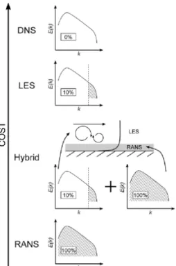
Accounting for the effect of turbulence on the flow field is done by either resolving or modeling the turbulence. Resolving spatially and temporally simulates the eddies themselves while modeling treats the turbulence as a set of statistics that describe the effects of turbulence. Methods for factoring turbulent effects on flow fields can be generally divided into three categories. In order of increasing computational complexity, they are Reynolds-Averaged Navier-Stokes (RANS), Large Eddy Simulation (LES), and Direct Numerical Simulation (DNS). Figure 1.2 shows the divide between resolving and modeling for each turbulence model in the context of the energy spectrum. The shaded regions on the energy spectrogram are modeled while the un-shaded regions are resolved. DNS uses the exact Navier-Stokes equations to solve a flow field and resolves the entire turbulence spectrum. The lack of modeling means that the spacial and temporal scales must be fully resolved by the mesh resolution and time-step size, respectively. These scales are defined by the Kolmogorov scales, which are very small, and thus significantly increases the computational cost associated with DNS. This cost results in DNS being used exclusively for research and only for simplified, lowRe flows. In fact, DNS is most commonly used to validate the modeling used in the other two categories.

Figure 1.2: Visualization of the different turbulence models and how they resolve or model the turbulence in the flow. The smaller plots show the energy cascade similar to Fig. 1.1. The shaded regions are modeled, non-shaded are resolved. This also shows the relationship between RANS and LES in HRLMs, which is further discussed in Section 1.2.3. Reproduced from [9] under the Creative Commons Attribution License (https://creativecommons.org/licenses/by/4.0/).

the turbulence at smaller scales using what are called sub-grid scale (SGS) models. Specifically, LES models the inertial scales of the turbulence, which contain the majority for the turbulent kinetic energy in the flow. While not as accurate as DNS, LES offers significant computational expense savings as the spacial and temporal resolution requirements are significantly reduced compared to DNS while still simulating the coherent structures of turbulence. LES may be used in industry in limited cases. While LES is less computationally expensive than DNS, it is still too expensive for most applications. Most of this expense is due to the spacial and temporal requirements in the boundary layer. The inertial scales, which must be resolved, are generally large, but near walls they decrease drastically. This increase in resolution in the near-wall-region accounts for a significant portion of the cost associated with LES.

RANS attempts to fully model the effect of turbulence on the flow field. It uses the result of taking the average of the Navier-Stokes equations while applying Reynolds decomposition to the flow variables (pressure and velocity). Reynolds decomposition separates an instantaneous variable into an average value and a fluctuating value:

Uj =Uj+uj (1.6)

Compared to LES or DNS, RANS is significantly more computationally cost effective. This is due primarily to the lack of significant grid requirements as well as the ability to directly calculate a steady state solution (so no temporal discretization is required). The only grid requirements for RANS are related to reducing the numerical error associated with the spacial discretization of the flow field, rather than physics-based constraints of the turbulence modeling method. RANS is not accurate for certain flow regimes. For example, for massively separated flows, RANS generally under-predicts the Reynolds stresses, changing the behavior of the separated wake region. However, many RANS models have been fine-tuned to be very accurate in simulating boundary layer flows, including prediction of separation points.

Turbulence Models and Swirl Swirl flows can have a significant effect on the accuracy of turbulence models. It is well known that linear eddy-viscosity based RANS models are insensitive to rotation in flows [10]. These models treat turbulence as an isotropic property while swirl’s effect is inherently anisotropic. Conversely, second-moment closure RANS models, also known as

Reynolds stress models (RSMs), treat turbulence as anisotropic property and do not suffer from this insensitivity. However, RSM is also an significant increase in computational cost compared to linear eddy-viscosity models and is known to be much more difficult to converge (ie. less robust). Corrections have been devised for linear eddy-viscosity models, such as [11], but they are obviously not perfect in their correction. LES and DNS techniques, like RSM, do not suffer any insensitivities to swirling flows. As previously mentioned though, these are significantly more computationally expensive than RSM, but are generally more accurate.

1.2.3

Hybrid RANS/LES Methods

The computational expense difference between LES and RANS is quite significant, but there are certain flows for which RANS is simply not accurate enough for. To fill the gap between these two models, hybrid RANS-LES methods/models (HRLMs) have been developed, with the basic premise being to use LES where accuracy is desired and RANS where LES is too expensive, as shown in Fig. 1.2. There are two different basic methods of implementing a HRLM: zonal and non-zonal.

In the zonal method, the RANS and LES areas of the domain are defined explicitly by the user before computation. Defining these zones requires knowledge of the flow field before the simulation is run to position the regions well.

Non-zonal methods choose when to transition from RANS to LES. Since much of the cost associated with LES comes from resolving the boundary layer, these methods will use RANS in the near-wall region and LES for the free stream. The determination of when this transition occurs is generally a function of wall height and mesh size, among other values. This method is very simple to implement as no prior information about the flow field is required. Non-zonal methods are more popular than zonal methods as defining RANS and LES zonesa prioriis non-trivial, particularly in flows with growing boundary layers, flow separation caused by adverse pressure gradient, and flow reattachment.

For non-zonal methods, the major challenge is choosing how and where to transition from RANS to LES. On the question of how, the challenge stems from translating the modeled turbulence in RANS into the resolved turbulence of LES. This is known as the grey area problem. On the question of where to transition, algorithms must decide based on mesh size and the wall height within the boundary layer. If this transition occurs too late, then the accuracy of LES is lost. If it occurs too early, the grid resolution may not be sufficient enough for LES to operate accurately.

Insufficient grid resolution causes an under-prediction of turbulent Reynolds stresses. This issue is called modeled-stress depletion (MSD). MSD can lead to a premature wall separation, which is called grid-induced separation (GIS).

The first non-zonal HRLM to was proposed by Spalart et al. [12] and was later implemented as the seminal detached eddy simulation (DES). This initial implementation suffered from an over-sensitivity to the mesh size when determining where RANS-LES transition should occur; if a mesh was over-refined near a wall, the RANS-LES transition would occur too soon (inside the boundary layer), leading to MSD. This was addressed by Menter and Kuntz [13] by using the boundary layer transition algorithm already implemented ink-ω SST (which operates under a similar principle as DES; use different models for near-wall area vs free stream). The model presented by Menter and Kuntz [13] used k-ω as the underlying RANS model and the technique was then generalized for use with any underlying RANS model by Spalart et al. [14], where it earned the moniker delayed DES (DDES). Several other proposed incremental improvements have been made, but will not be reviewed here.

1.2.4

Relevant Application of Computational Methods

Several numerical investigations of diffusers, both conical and non-conical, and swirling flows have been previously. Some relevant ones will be reviewed here.

Swirling Flows Dellenback et al. [15] recorded and published experimental data for high swirling flows in a pipe entering a cylindrical plenum. They performed the experiment at several different levels of swirl, ranging from Sr = 0 to Sr = 1.2. Several investigations of applying HRLMs to swirl flows have used these results as a validation case. The first is by Paik and Sotiropoulos [16], who compared the DDES model, using Spalart-Allmaras as the underlying RANS model, with experimental values and found good correlation. This comparison was done again by Javadi and Nilsson [17], who also added the improved DDES (IDDES) model into the comparison. They also found good correlation from the pair of HRLMs.

Diffusers The ERCOFTAC used a pair of 3-D rectangular diffusers as a test case for its 13th and 14th Workshop on Refined Turbulence Modeling [18, 19]. The experimental data used was gathered by Cherry et al. [20]. Both sets of diffusers exhibited wall separation, but of different characteristics

and degrees of severity. Participants in either workshop used a wide variety of turbulence models, from linear-eddy-viscosity RANS models to full LES. Overall, findings showed that HRLM or LES methods were required to fully resolve the mean flow features. Only a few RSM methods were reasonably accurate, while none of the linear eddy-viscosity models were able to correlate with the experimental data.

Several numerical investigations of conical diffusers with swirl have been performed previ-ously. Some used linear eddy-viscosity models, which are known to be problematic for these types of flows [21, 22]. Armfield et al. [23] and Cho and Fletcher [24] found success using algebraic RSMs to model swirling flows. From et al. [25] used the ERCOFTAC diffuser data from [1] as a validation and base for testing real-gas effects in this application. They used an explicit algebraic RSM (EARSM) and found decent success with that methodology. Sentyabov et al. [26] used the ERCOFTAC diffuser data and the Dellenback et al. [15] data to compare different turbulence models in swirling flows. They found that the RANS models tested, even with curvature corrections, weren’t accurate enough to model key flow characteristics. However, they did find good correlation to the experimental data from their DES model. Duprat et al. [27] performed a full LES analysis on ERCOFTAC conical diffuser data. They used a one transport equation SGS model to allow for a coarser grid. They also used a wall-modeled approach to reduce the computational costs of the simulation. The results of the simulation correlated well with the ERCOFTAC experimental results.

Chapter 2

Models & Methods

In this chapter, an overview of the methods used and the reasoning behind them for this research will be given. These methods will form a black-box function of the swirling flows of conical diffusers. This function has three inputs: two diffuser geometry constraints and the swirl strength at the inlet. The diffuser geometry constraints can be two ofAR, L/R1, andφ. By adjusting the constraints and observing the results, the relationship between the constraints and the output can be inferred.

2.1

Grid Generation

For creating the mesh for the model, a choice between the structured hexahedral mesh and an unstructured tetrahedral/polyhedral mesh was made. Unstructured tetrahedral/polyhedral has the benefit of more consistent element sizing throughout the domain, but can suffer from quality issues (skewness of elements being a key parameter). The structured hexahedral mesh takes more effort to create a suitable mesh, but the mesh quality is significantly higher compared to the unstructured. Thus, the structured hexahedral mesh was chosen.

There are several different ways to morph a structured grid onto a cylinder. An straight-forward way would be to simply create a structured 2-D mesh of the cylinder cross section and then rotate this around to form the cylinder. This would however leave elements in the center with a very high aspect ratio (ie. very thin in theθdirection compared to thezandr). Another way, which is what was done in this study, is to create what is called an O-grid, where the center of the cylinder

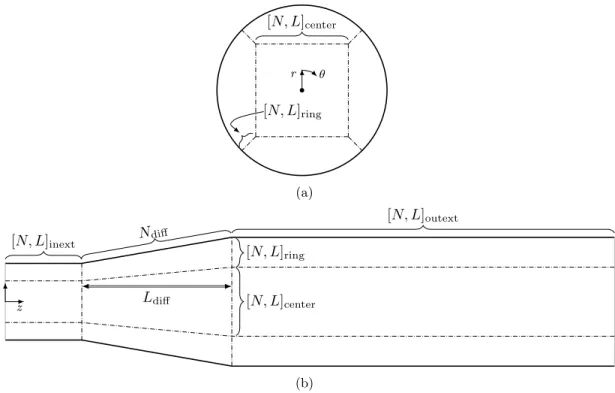
[N, L]center [N, L]ring r θ (a) [N, L]inext Ndiff Ldiff [N, L]outext [N, L]ring [N, L]center r z (b)

Figure 2.1: This diagram shows the mesh/domain parameters from (a) the inlet face and (b) a side view. N−represents the number of elements along the mesh framework edge whileL−represents the physical length of that edge. Theinext andoutext denote the inlet and outlet extension, respectively. Also notice in (b) the separation ofNdiff from Ldiff to keep the diffuser length consistent with the standard diffuser geometric definition.

is a standard hexahedral grid and the outer ring is an extrusion of that. This forms 5 total blocks: a single center block and 4 ring blocks. These blocks can be seen in Fig. 2.1a. This surface mesh is then extruded through the domain, forming the 3-D hexahedral elements. This type of mesh allows for finer control of the wall normal sizing, more consistent element sizing, and more isotropic cell sizes. This was the method used in this research.

The mesh is controlled through the number and distribution of elements on the edges of the blocks. The edges that are radially symmetric have the same distribution and number of elements. This reduces the number of edges that must be specified to 5, which are shown in Fig. 2.1.

For the length parameters of the mesh,Ldiff is determined by diffuser geometry andLinext andLoutext are determined by computational modeling constraints (which will be discussed in later sections). Conversely, Lring and Lcenter are determined to maximize mesh quality. TheLring and

Lcenter are inherently dependent on each other, though Lring is the most sensitive and will be the one directly specified here. Ideally, Lring this should be as small as possible, around the height of

the boundary layer. This would maximize the number of isotropic elements in the free stream of the domain. However, the smallerLring gets, the more skewed the elements at the corner of the center block become. These setup a tradeoff which must be addressed.

The overall goals for the mesh were to resolve the boundary layer to the viscous sublayer (ie. y+ _{<1) and to have the inner mesh cells be as isotropic (cubic in the case of hexahedral) as} possible. To resolve the boundary layer, the elements in the ring blocks are placed with a geometric distribution at a rate of around 1.2. The initial O-grid mesh at the inlet is swept down the length of the domain. In the diffuser portion of the geometry, the distribution of the sweep was increased at a constant rate to keep the core hexahedral cells as close to isotropic as possible.

2.2

Computational Setup

2.2.1

Turbulence Model

It is clear that eddy-viscosity-based RANS models are a poor choice for swirling flows (see Turbulence Models and Swirl in Section 1.2.2 for more details). While second-moment closure RANS models do not suffer from the same insensitivities that eddy-viscosity models do, they still suffer issues in wall-separated flows, such has those found in the ERCOFTAC Refining Turbulence Model workshops [18, 19] (see Diffusers in Section 1.2.4). In contrast, LES and HRLMs show very good correlation to experiments in these flow regimes. LES is, however, inhibitively expensive for wall-bounded flows, so HRLM was determined to be best option for this research.

There are two primary issues to consider when choosing a HRLM: grey area mitigation and modeled-stress depletion. MSD is well addressed with recent developments in HRLMs, while grey-area mitigation is still a topic under significant research [28, 29]. Since one of the significant flow regimes for conical diffusers is wall-separation, the transition of going from modeled to resolved turbulence is very important. ANSYS’s stress blended eddy simulation (SBES) has been shown to make this transition the fastest of all the HRLMs available in Fluent [30] and is also the recommended model for non-zonal HRLMs [31]. The recommended SGS model used is the wall-adapting local eddy-viscosity (WALE) model [32]. Note that Fluent’s sets the model constant Cw at 0.325 by default instead of the model’s original 0.5. The RANS model used was k-ω SST [33] with the curvature correction term added [11]. All other options or model constants were left to their default values.

2.2.2

Boundary Conditions

Outlet and Walls The outlet and wall boundary conditions are straight-forward. The walls are stationary and have a no-slip condition applied to them. The outlet is a static pressure outlet set to atmospheric pressure (101,1325 Pa) and has a non-reflecting condition set to prevent pressure waves from propagating upstream.

Inlet It is very important to have physically accurate profiles of velocity and turbulence at the inlet boundary condition. For that reason, the experimental data presented by Clausen et al. [1] will be used as the boundary condition for this research as it contains both velocity and Reynolds stress profiles. These experimental profiles will then be scaled to the boundary conditions required. This also means thatR1 will set to 130 mm to match the experiment setup. More detailed information about the experiment is given in Section 3.1.

To adjust the mean swirl levels of the experimental data, the Uθ profile will simply be multiplied by a scalar value. The determination of whether to scale Uz is a matter of choice. It could be scaled to keep the velocity magnitude, and thus the dynamic pressure, identical between different swirl rates. However, conical diffusers theoretically only transform the axial kinetic energy into pressure. It has been found that axial velocity reduces more than the circumferential velocity in a diffuser [7], with the reduction inUθattributed to conservation of angular momentum. Additionally, many applications generate higher axial velocities at operating regimes with swirling flows compared to operating regimes with pure axial flow. Therefore, it was determined to keep the axial velocity constant for all swirl types.

The Reynolds stresses in the ERCOFTAC data give information about the turbulence, but these Reynolds stresses cannot be directly given as the boundary conditions for the computational model. They must be translated into the turbulent quantities that are solved for by the turbulence model: turbulence kinetic energy,k, and specific turbulent dissipation rate∗, ω.

The definition ofkis given in Eq. (2.1) in index summation notation and expanded into the individual Reynolds stresses. This can be calculated directly from the Reynolds stresses given for the ERCOFTAC data.

k= 1 2ujuj = 1 2 u2 r+u2θ+u2z (2.1) ∗_{This term may also be known as the turbulence eddy frequency due to it’s units of s}−1

Conversely,ω cannot be derived directly from the ERCOFTAC data, so more information must be provided to close the solution. There are several different definitions forω. One of them is simply the ratio of k to the turbulent dissipation rate, ε: ω = ε/k†. This definition is where the name derives from. There is not a direct way to calculate ε from the Reynolds stresses. This quantity is also difficult to make a well-justified assumption on, so a different definition for ω is needed. The definition used for defining the turbulence quantities at the inlet boundary condition is given in Eq. (2.2)

ω= √

k

` (2.2)

where ` is the characteristic turbulence length scale. ` is the only unknown in the equation, and thus must be provided to closeω. The`can be given as a characteristic length scale of the flow. For example, in fully developed pipe flow` can simply be the diameter of the pipe. For flows through perforated plates,`can be set to the size of the perforations [35]. To generate the solid-body swirl, Clausen et al. used a sheet of honeycomb extrusion that had 3.2 mm holes [1]. Gyllenram and Nilsson [36] used this value to set`as a constant for the whole inlet. While this could also be done here, the characteristic length scale is known to reduce near the wall, as there simply isn’t enough space for the eddies to exist. This change in length scale can be approximated using Prandlt’s mixing length model. Near the wall, the mixing length is given as `mixing = κyw, where κ is the Von K´arm´an constant andyw is the wall height. κhas been experimentally found to be ≈0.4. To define`, and thus closeω, we set`=`mixingfor`mixing ≤3.2 mm, and`= 3.2mm for all otheryw. This is shown in Eq. (2.3). `=            κyw yw≤ 3.2 mm κ 3.2 mm yw≥ 3.2 mm κ (2.3)

Using Eqs. (2.2) to (2.3),ω was calculated using Eq. (2.4).

ω=            √ k κyw yw≤ 3.2 mm κ √ k 3.2 mm yw≥ 3.2 mm κ (2.4)

Adjusting Inlet for Swirling To isolate the effect of swirl on the conical diffuser, the inlet turbulence profiles should change as the swirl is changed as well. While the Reynolds stress profiles could be used as along side k and ω as inlet boundary conditions at the experimental swirl level, it is not known how to scale them accurately as the swirl is changed. Therefore the Reynolds stress profiles are not used directly for the inlet boundary condition. Note that this does reduce the physical realism of the inlet boundary condition and is further addressed in Section 2.2.3.

So how do we go about scaling kandω based on the swirl? Since only the circumferential velocity is being scaled, the maximum velocity magnitude changes with different swirl strengths. To reduce the effect of turbulence on the flow (in order to isolate the effect of swirl on the flow),kwill be scaled to keep the turbulence intensityIconstant. I is defined as

I= p ujuj kUk = p 2/3k kUk (2.5)

where kUk is the magnitude of the mean velocity and p

ujuj is the average magnitude of the fluctuating velocity. The latter term can be rewritten in terms ofk, which is seen in the third term of Eq. (2.5).

To keepI constant, the original and scaled quantities were set equal to each other, as seen in Eq. (2.6). The orig and scal subscripts represent the ERCOFTAC experimental data (original) and the scaled data, respectively.

Iorig=Iscal =⇒ p 2/3korig kUorigk = p 2/3 kscal kUscalk (2.6)

kUorigk and korig are known from the experimental data. kUscalk is also known from the desired level of swirl. The only unknown iskscal. By rearranging Eq. (2.6), we can solve forkscal:

kscal= 3 2 " kUscalk p 2/3korig kUorigk #2 (2.7)

Findingωscal is done using Eq. (2.4), replacingkforkscal:

ωscal =            √ kscal κyw yw≤ 3.2 mm κ √ kscal 3.2 mm yw≥ 3.2 mm κ (2.8)

0.85 0.90 0.95 1.00 r/R1 0 20 40 60 80 k / (m 2/ s 2) Interp Exp (a) 0.85 0.90 0.95 1.00 r/R1 0 2000 4000 6000 ω / s − 1 Interp Exp (b)

Figure 2.2: The 1-D cubic spline interpolation of (a) turbulent kinetic energy and (b) specific turbulent dissipation rate from the ERCOFTAC data. Circles represent the data computed from the experimental data and the lines are the interpolated data

The ERCOFTAC data is given along a single radial line. To input the data into Fluent, this data needed to be turned into cartesian points for the domain’s inlet surface. Several difficulties were had in using Fluent’s built-in surface interpolation algorithms, so the data was interpolated in 1-D (alongr) before being translated into 2-D cartesian coordinate points. To aid in this interpolation, wall values were added to the data. These were set asUi= 0 andk= 0 at the wall. The latter also causesω = 0 at the wall by definition. A cubic spline method was used for the interpolation. The results of the interpolation can be seen in Fig. 2.2. This 1-D data was then rotated around the inlet to create the 2-D cartesian data required by Fluent.

2.2.3

Inlet Turbulence Generation Methods

To mimic the ERCOFTAC experiment, the flow at the inlet of the diffuser must be turbulent. The inlet boundary conditions values given in the ERCOFTAC are time-averaged statistics. These statistics must be turned into physical and temporal velocity fluctuations for the LES portion of the domain to operate correctly.

Ideally, these fluctuations should perfectly resemble natural turbulence. It is possible to take well-resolved turbulence from a prior simulation and use it as the inlet boundary condition. This is difficult to do correctly and is very time intensive. It is easier to spontaneously generate turbulent fluctuations using an algorithm. Since it is planned to run several LES simulations, which alone are very computationally intensive, synthetic turbulence generator (STG) algorithms will be

used.

Creating random “noise” that has the same statistical quantities as the turbulent flow that is trying to be imitated is non-trivial. However, these fluctuations do not have the same physical coherent structures that characterize natural turbulence. Therefore, specific turbulence generator algorithms must be used to get as close to “real” turbulence as possible. The two main goals of STGs is to represent the statistical quantities input to them and form the coherent structures that characterize turbulence as quickly as possible.

In ANSYS Fluent, the available STG methods are vortex method and spectral synthesizer. The spectral synthesizer is an implementation of the technique presented by Smirnov et al. [37], which creates random vector fields that that are free of divergence based on Fourier harmonics. These vector fields represent the “noise” velocity fluctuations present in turbulence.

The vortex method was first proposed by Sergent [38]. It creates vortices at the inlet, where the size and strength of these vortices is determined by the boundary conditions k and ε. Since turbulence manifests itself as vortices, it is much closer to the “natural” turbulence than would be found in a simpler statistical method. In [38], the properties of the vortex were updated at discrete characteristic time steps. This was later improved by Mathey et al. [39] to allow the vortices’ properties to be updated more often. This is the method that is implemented into Fluent.

Vortex method was chosen as it creates the chaotic fluid motions of turbulence in a physically coherent structures. Because of this, it transitions into natural turbulence more quickly than Fourier-based methods, such as the spectral synthesizer [40].

As stated in the previous section, the Reynold’s stress data were not used to define the inlet boundary condition. All of the STGs in Fluent can use the Reynolds stress to further define the turbulence it generates. Not using these Reynolds stresses does reduce the physical realism of the simulation as the anisotropic turbulence that is a characteristic in swirling flows is no longer produced at the inlet. The anisotropy will instead be recovered as the synthetic turbulence transforms into natural turbulence [39].

The “traditional” recommendation for the appropriate length to transition from synthetic to natural turbulence is around 3–5 boundary layer thicknessesδ. This only accounts for isotropic turbulence however. To ensure that the anisotropic turbulence is recovered before reaching the diffuser inlet, an entrance length of∼10δ is targeted.

2.2.4

Other Computational Setup Details

The initial conditions for the model come from the results of a RANS simulation usingk-ω

SST with the curvature correction scheme. The ‘init-instantaneous-vel’ command in Fluent is then used to generate a dynamic velocity field from these stead-state results using a synthetic turbulence generator (Fluent does not disclose what STG is used for this operation). This initializing simulation as well as the SBES simulation are done using an incompressible solver.

SBES is an transient simulation, but the quantities of interest are desired to be time-averaged. Thus an averaging process is used (this process also gathers other statistics, such as resolved Reynolds stresses and RMS values of velocity and pressure). However, the simulation starts with RANS results and synthetic turbulence and taking the average of these artificial results will add noise to the actual results. Thus a start-up period is used before the averaging process is started. To determine the start up time, the flow-through time, or time taken for a particle to go from inlet of the domain to the outlet, is generally used. For these simulations, 3 flow-through times were used before averaging was begun. Convergence for the simulation was determined by analyzing the history of specific monitor points in the simulation. As more time-steps are used for the average, the results begin to converge onto the steady-state value.

Numerically, the temporal discretization was performed using a bounded second-order im-plicit method. SIMPLEC was used as the pressure-velocity coupling scheme. The default under-relaxation factors were increased to accelerate convergence. The pressure and momentum terms were solved with second-order and bounded central difference, respectively. The turbulent quantity equa-tions,kandω, used a first-order upwind scheme. All these choices were made on recommendations from Menter [31].

While generally the Courant-Friedrichs-Lewy (CFL) condition is a stability condition, the use of an implicit temporal scheme makes the simulation unconditionally stable. Thus the CFL condition, and it’s associated Courant number, is used to ensure accuracy in the solution. The Courant number was kept below 10 for the RANS domain and below 1 for the LES domain, per recommendations of Menter [31].

Chapter 3

Validation

3.1

Overview of Validation Method

To validate the computational model used for this research, simulations were performed to compare to experimental results. The experiment chosen was performed by Clausen et al. [1]. The data from this experiment has been made available through the ERCOFTAC database; thus this data will be referred to as the “ERCOFTAC diffuser”. The experiment was of a conical diffuser with solid-body inlet swirl. The swirl was generated using a honeycomb mesh (size 3.2 mm) mounted on a rotating pipe that was 400 mm in length. A fine mesh was used upstream of the honeycomb to reduce the boundary layer height before entering the diffuser. After the rotating wall, there was a 100 mm stationary section before entering into the diffuser. These dimensions can be seen in Fig. 3.1. The dimensions of the diffuser were a half-angle φ = 10◦, length Ldiff = 510 mm, and an inlet radius R1 = 130 mm. This results in an AR of 2.862. The swirl number of the flow was Sr = 0.298. The data was collected by hot-wire anemometers in an X-probe and single wire configuration operating in a constant-temperature mode. This experimental data set includes axial and circumferential velocity profiles, Reynolds stress profiles, and pressure distribution at the diffuser walls. The profiles were taken at different ‘stations’ which can be seen in Fig. 3.1. Notice that Clausen et al. used a coordinate system normal to the wall for data collection in the diffuser section. The results from the simulation were translated into this coordinate system for comparison purposes. These altered coordinate systems are denoted with a superscript star: U_z∗, y∗_w, z∗. The exact definitions for the altered dimensions is shown in Eqs. (3.1) to (3.3). Note that the definition

forθandUθdo not change with the new coordinate system. z∗=        z−Linext z≤Linext z−Linext

cosφ Linext < z≤Ldiff

(3.1) y∗_w=        R1−r z≤Linext R1−r

cosφ Linext< z≤Ldiff

(3.2) U_z∗=        Uz z≤Linext

Uzcosφ+Ursinφ Linext< z≤Ldiff

(3.3)

Clausen et al. non-dimensionalized the experiment data using characteristic experiment values. They defined a velocity U0 which is approximately the area-average of Uz at the diffuser inlet: 11.6 m s−1_{. The velocity data has been non-dimensionalized by U}

0 and the Reynolds stress data by U2

0. The wall pressure distribution is given by Cp, which is the static pressure divided by some reference dynamic pressure: Cp = p/q = p/(12ρkUk

2_{). Clausen et al. utilized U}

0 in the definition of their reference dynamic pressure, as seen in Eq. (3.4). This non-dimensionalization will be done in this validation as well.

Cp= p 1 2ρU 2 0 (3.4)

For the dimensions of the computational domain itself, the diffuser geometry inherently defines all but theLinext, Loutext, and Lring (see Fig. 2.1 for dimension parameters). TheLinext is chosen based on the location of where the experimental inlet data was collected and on the entrance length required for the synthetic turbulence to transition to natural turbulence. The data was collected 25 mm downstream of the diffuser. The target entrance length is∼10δ(see Section 2.2.3) and the approximate boundary layer height is 20 mm. Combined this leads to an estimated 225 mm for theLinext. This is rounded up to 260 mm to get an even 2R1 length. ForLoutext, 1300 mm, or 10R1, was used to ensure adequate distance between the output boundary condition and the diffuser section. Lring was determined to be best if set to 30 mm as a balance between fully resolving the boundary layer and minimizing skewed elements in the corners of the center block.

rz y_w∗

z∗

Rotating Walls Stationary Walls

400 mm 100 mm 510 mm 130 mm -25 25 60100 175 250 330 405 Honeycomb

Figure 3.1: Diagram of the experiment setup used in Clausen et al. [1]. Lines of show the measurement stations, with their associated z∗ value displayed above in mm. Also shown is the rotating walls and stationary walls .

Nring Ncenter Ninext Ndiff Noutext Total Cells

50 42 80 120 180 3.6 million

Table 3.1: Parameters of the baseline mesh used in initial model validation. The mesh size param-eters are based on the terms shown in Fig. 2.1.

mm upstream of the diffuser. This data is used at the inlet of the domain, 260 mm upstream of the diffuser. Since the walls of the inlet extension are stationary, this will change the flow conditions at the inlet of the diffuser compared to the experiment. An idea to avoid this would be to make part of the inlet extension wall rotate, much like in the experiment. However when compared with stationary walls, this may distort the inlet profile unpredictably as theUθ boundary layer will begin to recover in the rotating region and then start growing again once it hits the stationary walls. This back-and-forth causes an unknown distortion to the inlet conditions. Conversely, having stationary walls causes predictable changes to the flow conditions that can be accounted for when examining the results.

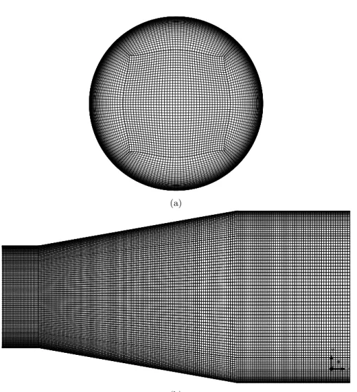
The largest grid size was chosen to be equal to of the turbulence length scale. The first layer height at the wall was set at 0.02 mm and was chosen based on preliminary RANS simulations to target a y+ _{< 1. The distribution of elements in the near-wall region has been described in} Section 2.1. The parameters for this mesh are given in Table 3.1. Images of the mesh are given in Fig. 3.2.

Z Y X (a) X Y Z (b)

Figure 3.2: A view of the (a) inlet and (b) side of baseline mesh. Note that while the cells appear to be rectangular from the side, the cells on the inside of the mesh are closer to isotropic size.

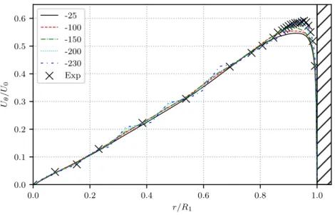
0.0 0.2 0.4 0.6 0.8 1.0 r/R1 0.0 0.1 0.2 0.3 0.4 0.5 0.6 Uθ /U 0 -25 -100 -150 -200 -230 Exp

Figure 3.3: Plots of Uθ at different z∗ locations in the inlet extension. The hatch at r/R1 = 1 denotes the wall of the inlet extension. Note that the inlet boundary condition face is -260 mm from the diffuser inlet. A more detailed view of the near-wall region is presented in Fig. 3.4

3.2

Validation Results

3.2.1

Inlet Conditions

Before looking at the results in the diffuser section, a comparison between the experimental and computational inlet conditions is done. As previously mentioned, the inlet pipe of the diffuser is a stationary wall, causing the velocity profiles from the ERCOFTAC diffuser data to alter before they reach -25 mm aft of the diffuser inlet. Figure 3.3 shows the progressive change in the computational

Uθprofile at selectz∗distances from the diffuser inlet. The profile away from the wall stays relatively unchanged throughout the inlet extension. Most of the velocity change occurs in the boundary layer, which is seen better in Fig. 3.4. Near the wall, the profile is very close to that of the experiment, but the peak quickly decreases.

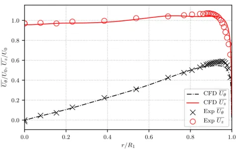
The axial velocity progression did not show any significant deviation from the experimental values. Both velocity component profiles for the inlet of the diffuser are presented and compared to experimental values in Fig. 3.5. The simulation results show differences in the boundary layer shape, but over all the convergence is reasonably close to the original results. ComputingSrat the -25 mm station gives a value of 0.289 compared to the ERCOFTAC value of 0.298; a 3% drop in swirl strength.

0.800 0.825 0.850 0.875 0.900 0.925 0.950 0.975 1.000 r/R1 0.400 0.425 0.450 0.475 0.500 0.525 0.550 0.575 0.600 Uθ /U 0 -25 -100 -150 -200 -230 Exp

Figure 3.4: A detailed look at theUθ profile in the near-wall region at differentz∗ locations in the inlet extension. The hatched area represents the inlet extension wall.

0.0 0.2 0.4 0.6 0.8 1.0 r/R1 0.0 0.2 0.4 0.6 0.8 1.0 Uθ /U 0 , Uz /U 0 CFDUθ CFDUz ExpUθ ExpUz

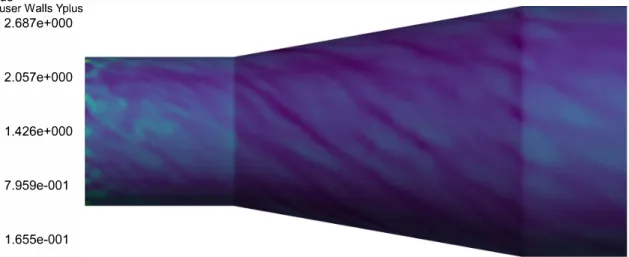
Yplus

Diffuser Walls Yplus

2.687e+000 2.057e+000 1.426e+000 7.959e-001 1.655e-001

�

z

Figure 3.6: y+ contour plot on walls.

3.2.2

Computational Model Checks

There are a few other checks to make sure the computational model is working correctly. The first isy+_{, which is shown in Fig. 3.6. Most of the walls of the domain havey}+ _{<1, with the} only exceptions being in the inlet extension.

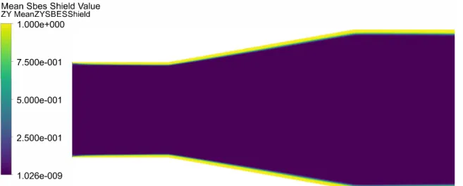
The other main check is of the SBES shielding function, fSBES. This function determines whether the HRLM should operate in RANS mode (fSBES= 1) or in LES mode (fSBES= 0). The transition between 1 and 0 is the ”blending” in stress blended eddy simulation. This function can be plotted to ensure that the HRLM is using RANS or LES in the correct regions. The value for

fSBES is plotted in Fig. 3.7. We can see that the model is using RANS for the near-wall region and then quickly transitioning to LES in the free stream. Additionally, we can see that the RANS area grows as the flow moves downstream, matching the increasing boundary layer height.

Lastly, the Courant number will be looked at. The targets for HRLMs are Courant number

<1 for the LES region and<10 for the RANS region. A plot can be seen in Fig. 3.8. The entire domain is kept below 1 except for small portions near the wall of the inlet extension. These areas are within the RANS region of computation and are within the limit set for it.

3.2.3

Diffuser Results

TheUz profiles at the 25, 175, and 405 mm stations are presented in Fig. 3.9. The overall correlation is good, except for the near-wall boundary layer region. This discrepancy is most likely

Mean Sbes Shield Value ZY MeanZYSBESShield 1.000e+000 7.500e-001 5.000e-001 2.500e-001 1.026e-009

�z

Figure 3.7: Contour plot of the SBES shielding function,fSBES. Function equals 1 when in RANS

mode and 0 when in LES mode.

Cell Convective Courant Number ZY 1.225e+000 9.193e-001 6.134e-001 3.075e-001 1.555e-003

�

z

Figure 3.8: Contour plot of Courant number in the domain.

0.0 0.2 0.4 0.6 0.8 1.0 1.2 1.4 1.6 y_w∗_/R1 0.0 0.2 0.4 0.6 0.8 1.0 Uz /U 0 CFD 025 CFD 175 CFD 405 Exp 025 Exp 175 Exp 405

Figure 3.9: Uzprofiles of the diffuser.

due to some deficiency in the k-ω SST turbulence model, as the boundary layer profile is better predicted by From et al. [25] using a RSM model.

The Uθ profiles are also plotted at the same stations in Fig. 3.10. The magnitude of the profiles is consistently under predicted, but the flow characteristics themselves are present. Specifi-cally, the “double-peak”, best seen in the 405 mm station, is captured by the simulation. Also note that the 405 mm station also has negative Uθ values. This indicates a shift in the rotation axis of the swirl.

The results of the simulation are compared to the experimental results in Fig. 3.11. The results generally correlate well. The general shape of the pressure distribution is nearly identical, including before the diffuser itself. The pressure is generally over-estimated though converges quite close to the experimental results, particular in the latter half of the diffuser.

An isosurface of Uz = 0 is shown in Fig. 3.12 to visualize recirculation regions, including wall separation and vortex breakdown. Clausen et al. [1] reported no internal recirculation or wall separation in the experiment itself. There is no wall separation present in the numerical results. There is a small internal recirculation region after the diffuser exit. It is unclear as to what difference between the experimental and numerical result has caused this.

0.0 0.2 0.4 0.6 0.8 1.0 1.2 1.4 1.6 yw∗/R1 0.0 0.1 0.2 0.3 0.4 0.5 0.6 Uθ /U 0 CFD 025 CFD 175 CFD 405 Exp 025 Exp 175 Exp 405

Figure 3.10: Uθ profiles of the diffuser.

−0.5 0.0 0.5 1.0 1.5 2.0 2.5 3.0 3.5 z∗_/R1 0.0 0.2 0.4 0.6 0.8 1.0 Cp CFD Exp

Chapter 4

Experiment

4.1

Design of Experiments

To find the relationship of geometry and swirl on diffuser performance, a series of simulations has been carried out. As discussed in Chapter 2, the computational model forms a black-box function with three inputs (two diffuser geometry, one swirl strength) and one primary output (performance). This forms a 3-D design space, with each function evaluation (simulation) forming a point in that design space. To ease the computational expense, we will hold one of the variables constant. Obviously, swirl strength cannot be kept constant to investigate the desired relationship, so one of the diffuser geometry inputs will be held constant. AsARhas the most significant effect on diffuser performance (as it sets theCP R,i for the geometry, see Eq. (1.2)), it is important that this variable not be held constant. Conversely,L/R1has the least significant effect on performance once the flow is devoid of any wall-separation. Thus,L/R1 will be held as a constant value. WithL/R1 constant,φandARhave the same effect on the diffuser geometry. We will adjustφexplicitly in this experiment. The adjustment of the swirl strength will simply be a multiplier of the ERCOFTAC diffuser data, as described in Section 2.2.2.

The design of experiment was chosen to be a 3×3 matrix of function evaluations, with three different values ofφand swirl multiplier. This results in 9 total function evaluations. To minimize extrapolation, the baseline run for the matrix was chosen to be the ERCOFTAC diffuser experiment setup. All other simulations in the matrix will be modifications from this baseline setup.

recirculation occurs. The diffuser geometry and boundary conditions in the ERCOFTAC diffuser close to having full internal recirculation [1]. Thus, increasing the swirl strength will cause internal recirculation to occur. The three swirl multipliers were chosen to be 100, 150, and 200 percent strength of the ERCOFTAC diffuser data. This corresponds to Sr = [0.298,0.447,0.596]. The three values forφwere chosen to beφ= [10◦, 12.5◦, 15◦], corresponding toAR= [2.86,3.50,4.21]. For the sake of brevity, each simulation will have a shortened name corresponding to its design variables. The naming convention is “p[φ×10]S[Sr×100]”. For example, the ERCOFTAC diffuser case used in the validation would simply be p100S298.

4.2

Results

To visualize the recirculation region of the diffusers, the isosurface of Uz = 0 has been plotted for the design points in Fig. 4.1. All of the diffusers exhibited some form of recirculation, though for the p100S298 case this occurs upstream of the diffuser itself. Even forφ= 10◦, the lowest swirl tested was sufficient to avoid wall separation. There are a few trends to point out. The first is that as the swirl increases, the point of vortex breakdown occurs farther upstream. This correlates with the findings of So [6]. The second is that asφis increased, the width of the recirculation region increases.

CPR will be used to determine the diffuser performance, defined in Eq. (1.1) and has been

reproduced below: CP R= p2,avg−p1,avg q1,avg = p2₁,avg−p1,avg 2ρkUk 2 1,avg (1.1)

The dynamic pressureq serves as the maximum pressure rise possible with the given flow. As the swirl level changes, kUk2

1,avg increases. However, theoretically, the conversion of kinetic energy to enthalpy (in the form of static pressure) should not change the rotational kinetic energy of the flow. In other words, Uθ does not contribute directly to the static pressure rise. Thus, the theoretical maximum pressure rise should not change with different levels of swirl. In other words, the denominator could alternatively be defined using the area-averagedUz at the diffuser inlet:

CPR,Uz = p2,avg−p1,avg 1 2ρU 2 z1,avg (4.1)

φ/◦ Sr

0.298 0.447 0.596

15

12.5

10

Figure 4.1: Isosurfaces ofUz= 0 to visualize the recirculation region of the flow. The diffuser walls are also shown in transparency.

Uz1,avgshould be constant and approximately equal toU0. A new definition forCPR can be defined

usingU0: CPR,U0 = p2,avg−p1,avg 1 2ρU 2 0 (4.2)

This will be the primary performance metric used. However, bothCPR,U0 and the original

definition for CPR, Eq. (1.1), will be shown for comparison. To further help distinguish the two

definitions, the original definition will denoted byCPR,q. Lastly, another note to make is that since the denominator remains constant inCPR,U0, the value corresponds linearly to the pressure rise.

Plotted in Fig. 4.2 is a contour plot of theCPR,U0 in the design space. The increasing swirl

has a significant negative impact on diffuser performance. Conversely, changing φhas a negligible impact on the diffuser performance. The only area in the design space that φ effects the diffuser performance occurs around p100S298. This is mostly likely because p100S298 operates at a different flow regime to all the other design points, as it has a negligible amount of internal recirculation.

Contours ofCPR,q are plotted in Fig. 4.3. The distortion in the p100S298 area of the design map is not as significant as in Fig. 4.2.

0.30 0.35 0.40 0.45 0.50 0.55 0.60 Sr 10 11 12 13 14 15 φ/ ◦ 0.400 0.500 0.600 0.700 0.800 0.4 0.5 0.6 0.7 0.8 CPR ,U 0

Figure 4.2: Contour ofCPR,U0. The design space points simulated are plotted as well. The color of

the dot corresponds to theCPR,U0 of the design point.

0.30 0.35 0.40 0.45 0.50 0.55 0.60 Sr 10 11 12 13 14 15 φ/ ◦ 0.300 0.400 0.500 0.600 0.700 0.3 0.4 0.5 0.6 0.7 CPR ,q

Figure 4.3: Contour ofCPR,q. The design space points simulated are plotted as well. The color of the dot corresponds to theCPR,q of the design point.

Chapter 5

Conclusion

To determine the static pressure recovery effects of swirl in conical diffusers, a computational model was created and validated utilizing hybrid RANS/LES turbulence models to accurately model the flow. The boundary conditions for the simulation were derived from the ERCOFTAC diffuser experiment performed by Clausen et al. [1]. A total of 9 simulations were completed to evaluate the design space. The parameters for these simulations were chosen to evaluate the diffuser performance behavior at swirl rates high enough to cause internal recirculation in the diffuser. It was found that at these high swirl levels where internal recirculation has occurred, geometry had little to no effect on the performance of the diffuser. In other words, once internal recirculation occurs, the diffuser performance becomes a function of swirl strength only.

Appendix A

Validation Plots

�

z

Mean Velocity ZY 1.434e+001 1.076e+001 7.176e+000 3.592e+000 8.834e-003 [m sA_-1]

�

z

Figure A.2: Contour of average velocity magnitude,kUk.

0 � � t5 0 ,+-J (]) 0 ·c3> + 0 >, Q) _ _,("f) Q) "t5 ("f) >o-q-C a, co> � Q) >-�N � 0 0 0 0 0 + + Q) Q) LO O') I'--c.o 0 � � I'--0 0 0 + Q) � O') LO ("f) N 0 0 I Q) ("f) LO ,... N � • I �< (/) E ...

Pressure. Trnavg ZY 6.139e+000 -1.830e+001 -4.275e+001 -6.719e+001 -9 .164e+00 1 [Pa] 0.400 (m)

�

z

Appendix B

Experiment Results

φ/◦ Sr CP R,q CP R,U0 p1,avg/Pa p2,avg/Pa q1,avg/Pa (p2,avg−p1,avg)/Pa

10 0.298 0.735 0.884 -75.60 -2.77 99.10 72.83 10 0.447 0.475 0.667 -67.00 -12.10 116.00 54.90 10 0.596 0.244 0.408 -51.90 -18.29 138.00 33.61 12.5 0.298 0.719 0.864 -77.30 -6.15 99.00 71.15 12.5 0.447 0.472 0.662 -67.89 -13.41 115.00 54.48 12.5 0.596 0.243 0.403 -52.67 -19.50 137.00 33.17 15 0.298 0.717 0.862 -77.92 -6.92 99.00 71.00 15 0.447 0.465 0.650 -67.20 -13.65 115.00 53.55 15 0.596 0.238 0.394 -52.68 -20.21 136.00 32.47

Table B.1: Results of experiment. For reference, dynamic pressure q referencing U0 is equal to 82.28 Pa.