BEHAVIOR OF TURBULENT STRUCTURES WITHIN A MACH 5 MECHANICALLY DISTORTED BOUNDARY LAYER
A Dissertation by
SCOTT JACOB PELTIER
Submitted to the Office of Graduate Studies of Texas A&M University
in partial fulfillment of the requirements for the degree of DOCTOR OF PHILOSOPHY
Chair of Committee, Rodney D. W. Bowersox Committee Members, Edward B. White
Othon Rediniotis Simon North
Head of Department, Rodney D. W. Bowersox
August 2013
Major Subject: Aerospace Engineering
ii ABSTRACT
High-resolution particle image velocimetry (PIV) is employed to resolve the velocity fields within a Mach 4.9 mechanically distorted turbulent boundary layer (Reθ ≈ 40,000).
The goal of this study is to directly observe the mechanisms responsible for the modified turbulent stresses present in mechanically distorted boundary layers. This is achieved by measuring the effects of the mechanical distortions upon the distribution, population, size, orientation, and energy content of the turbulent structures, and how the perturbed state of these structures is manifested within the ensemble-averaged turbulent stresses. The two mechanical distortions under investigation are 1) streamline curvature-induced favorable pressure gradients (Ip = {-0.08; -0.49}), and 2) periodic arrays of diamond roughness elements (k/δ ≈ 0.07). A smooth-wall, flat-plate boundary layer is also included to establish the unperturbed state of the turbulent structures. The response of the mean turbulence statistics is investigated through ensemble-averaged profiles of Reynolds stresses, indicating the respective influences of pressure gradient effects and surface roughness upon the turbulent statistics. The distortion and reorientation of the large-scale coherent motions is quantified through the determination of the integral length scale and local structure angle from two-point correlations. Detection of individual vortices through the swirling strength criterion λci allows the population distribution of the turbulent eddies to be examined, along with the conditionally averaged hairpin structure.
The baseline and rough-wall stresses showed good agreement when scaled by the smooth-wall friction velocity. Two-point correlations indicate that the reorientation of the large-scale [i.e. O(δ)] coherent structures, coupled with the modified wall-normal fluctuations, is primarily responsible for the modification of the rough-wall Reynolds stresses. The reduced Reynolds stresses observed in the favorable pressure gradients is partially due to the attenuation of the local flowfield around the near-wall hairpin
iii
structures, mitigating the mechanism for “producing” turbulence. The rotational rate of the hairpin vortices, measured through the mean prograde swirling strength, was reduced for the favorable pressure gradient models.
iv
ACKNOWLEDGEMENTS
I would like to thank my advisor, Dr. Rodney Bowersox, for his endless encouragement and boundless optimism throughout this project, and for granting me the freedom to expand the scope of my research into new and exciting areas. I would also like to thank Dr. John Schmisseur of the Air Force Office of Scientific Research (AFOSR) for financially supporting this endeavor.
I appreciate the technical assistance of Jorge Martinez, John Kochan, and the rest of the staff at the Oran W. Nicks Low Speed Wind Tunnel. Additionally, I would like to thank Will Seward for his machining expertise and general advice.
I would like to thank Dr. Isaac Ekoto, who was responsible for the design and construction of the facilities used during my Ph.D. program, and whose research inspired much of the work in this dissertation. I also appreciate the assistance of all the students at the National Aerothermochemistry Laboratory. Keeping the lab running is definitely a team effort, and I couldn’t have completed my research without their assistance.
Finally, I would like to thank Dr. Raymond Humble for his technical and scientific assistance, including the many spirited discussions that encouraged me to push the boundaries of my dissertation.
v TABLE OF CONTENTS Page ABSTRACT ... ii ACKNOWLEDGEMENTS ... iv TABLE OF CONTENTS ... v LIST OF FIGURES ... x LIST OF TABLES ... xxv 1. INTRODUCTION ... 1 1.1. Motivation ... 1
1.2. Overview of Mechanically Distorted Supersonic TBLs ... 4
1.2.1. Surface Roughness ... 5
1.2.2. Curvature-Driven Favorable Pressure Gradients (FPGs) ... 8
1.3. Research Framework ... 11
1.4. Scientific Approach ... 14
2. BACKGROUND REVIEW ... 17
2.1. Turbulent Boundary Layer Fundamentals ... 17
2.1.1. Coherent Structures in Turbulent Boundary Layers ... 17
2.1.2. Nomenclature of Coherent Structures ... 23
2.2. Favorable Pressure Gradient Effects ... 24
2.3. Surface Roughness Effects ... 29
2.3.1. Classical Scaling Laws ... 29
2.3.2. Compressibility Effects ... 32
3. EXPERIMENTAL FACILITIES & HARDWARE ... 35
3.1. NAL Laboratory Complex ... 35
3.2. Experimental Facility ... 36
3.2.1. Air Supply ... 37
3.2.2. Settling Chamber ... 38
vi
Page
3.2.4. Test Section ... 40
3.2.5. Diffuser ... 41
3.2.6. Exhaust Muffler ... 42
3.2.7. Tunnel Monitoring and Operating Conditions ... 43
3.3. Experimental Models ... 45
3.3.1. Periodic Roughness Model ... 45
3.3.2. Curvature-Driven Pressure Gradient Models ... 48
4. EXPERIMENTAL DIAGNOSTICS & ANALYSIS METHODS ... 53
4.1. Schlieren Imaging ... 53 4.1.1. Schlieren Principles ... 53 4.1.2. Continuous-Source Arrangement ... 56 4.1.3. Spark-Source Arrangement ... 59 4.2. PIV Principles ... 62 4.2.1. Tracer Particles ... 63 4.2.2. Imaging ... 65 4.2.3. Vector Reconstruction ... 66
4.3. PIV Experimental Arrangement ... 68
4.3.1. Flow Seeding ... 70
4.3.2. Illumination & Imaging ... 73
4.3.3. Vector Processing & Validation ... 75
4.4. Post-Processing and Analysis Methods ... 79
4.4.1. Ensemble-Averaged Profiles ... 80
4.4.2. Spectral Analysis ... 80
4.4.3. Quadrant Decomposition ... 82
4.4.4. Length-Scale Estimation ... 84
4.4.5. Conditional Averaging ... 86
5. VORTEX IDENTIFICATION TECHNIQUES ... 89
5.1. Vortex Identification Methods ... 89
5.1.1. Vorticity ... 90
5.1.2. Galilean Decomposition ... 91
5.1.3. Local Pressure Minimum (λ2 criterion) ... 94
5.1.4. Q-Criterion ... 96
5.1.5. Swirling Strength ... 98
5.2. Vortex ID Methods in Current Study ... 100
5.2.1. Implementation of Vortex Detection Algorithms ... 102
5.2.2. Compressibility Effects ... 102
vii
Page
5.2.4. Filtering of Detected Vortices ... 109
5.2.5. Mechanical Distortions Effects ... 113
6. CHARACTERIZATION OF BASELINE FLAT-PLATE, SMOOTH-WALL BOUNDARY LAYER ... 118
6.1. Flow Characteristics and Mean Velocity ... 118
6.2. Reynolds Stress Response ... 121
6.3. Spectral Distribution of Turbulent Energy ... 125
6.4. Spatial Distribution of Turbulent Energy ... 128
6.5. Instantaneous Structure of Near-Wall Flow ... 135
6.6. Vortex Motions and Population Distribution ... 145
6.7. Conditional Structure of Near-Wall Flow ... 157
6.8. Origin of Retrograde Vortices ... 165
6.9. Summary and Discussion of Results ... 170
7. BOUNDARY LAYER RESPONSE TO STREAMLINE CURVATURE-INDUCED FAVORABLE PRESSURE GRADIENTS ... 172
7.1. Mean Flow Response ... 172
7.2. Reynolds Stress Response ... 177
7.3. Spatial Organization of Large-Scale Structures ... 188
7.4. Instantaneous and Statistical Structure of Near-Wall Boundary Layer ... 199
7.5. Vortex Motions and Population Distribution ... 213
7.6. Conditional Structure of Near-Wall Boundary Layer ... 221
7.7. Discussion of Results ... 232
7.7.1. Length Scale Distribution ... 232
7.7.2. Shear Stress Attenuation ... 234
7.8. Summary ... 241
8. BOUNDARY LAYER RESPONSE TO PERIODIC SURFACE ROUGHNESS .... 244
8.1. Flow Visualization ... 244
8.2. Mean Flow Response ... 247
8.2.1. Wall-Normal Profiles ... 248
8.2.2. Streamwise Evolution ... 251
8.3. Reynolds Stress Response ... 253
8.3.1. Streamwise Evolution ... 253
8.3.2. Wall-Normal Profiles ... 257
8.3.3. Shear Stress-Producing Events ... 264
viii
Page
8.4.1. Two-Point Correlations ... 267
8.4.2. Streamwise Dependency ... 273
8.4.3. Spectral Content ... 276
8.5. Vortex Motions and Population Distribution ... 280
8.6. Conditional Structure of Near-Wall Boundary Layer ... 284
8.7. Discussion of Results ... 288
8.7.1. Reynolds Stress Scaling ... 288
8.7.2. Reynolds Stress Redistribution ... 290
8.7.3. Reorientation of Large-Scale Motions ... 294
8.8. Summary ... 296
9. SUMMARY ... 298
9.1. Undistorted (ZPG) Boundary Layer ... 299
9.2. Effects of Wall Curvature and Favorable Pressure Gradients ... 300
9.3. Effects of Periodic Surface Roughness ... 301
9.4. Contributions of the Current Study ... 302
9.5. Recommendations ... 303
9.5.1. Vortex Detection ... 303
9.5.2. POD Analysis ... 305
9.5.3. Form Drag of Roughness Elements ... 306
9.5.4. Vortex Stretching within Favorable Pressure Gradients ... 309
REFERENCES ... 311
APPENDIX A: WALL TEMPERATURE MEASUREMENT ... 323
A.1. TSP Principles ... 324
A.2. Experimental Arrangement ... 325
A.2.1. Calibration ... 325
A.2.2. Experimental Procedure ... 327
A.3. Measured Surface Temperature ... 328
APPENDIX B: UNCERTAINTY ANALYSIS ... 331
B.1. Instantaneous Velocity ... 332
B.2. Boundary Layer Thickness ... 333
B.3. Particle Slip Estimation ... 337
B.4. Velocity Gradients ... 340
B.5. Swirling Strength λci ... 341
ix
Page
C.1. Processing & Post-Processing Settings ... 344
C.2. Averaging Filter ... 346
APPENDIX D: SEEDER OPERATION MANUAL ... 348
D.1. Construction & Design ... 348
D.2. Procedures ... 350
D.2.1. Prior to Operation ... 350
D.2.2. After Tunnel has Started ... 350
D.2.3. Prior to Shutdown ... 350
D.2.4. After Tunnel Shutdown ... 350
APPENDIX E: SENSITIVITY OF VORTEX IDENTIFICATION TECHNIQUE ... 352
APPENDIX F: APPLICABILITY OF CROCCO-BUSEMANN RELATION TO NON-ZERO PRESSURE GRADIENTS ... 356
APPENDIX G: DECREASING BOUNDARY LAYER THICKNESS OVER SURFACE ROUGHNESS ... 358
x
LIST OF FIGURES
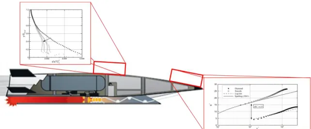
Page Figure 1.1 Schematic of a typical hypersonic vehicle, indicating potential areas for
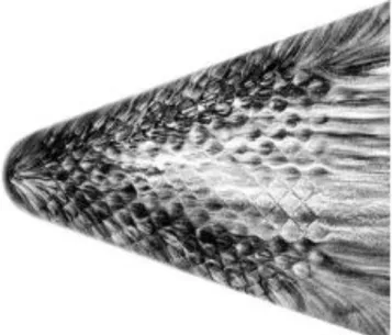
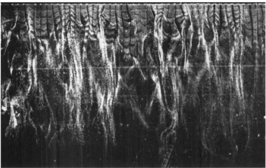
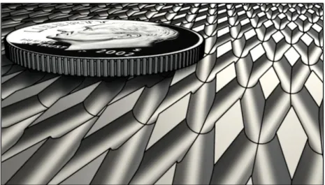
mechanical distortions. Image taken from Pratt and Whitney. ... 2 Figure 1.2 Examples of distributed roughness. ... 4 Figure 1.3 Cartoon describing “black box” analysis method for a turbulent
boundary layer ... 13 Figure 2.1 Conceptual drawing of a horseshoe or “hairpin” vortex. From
Theodorsen (1952) ... 19 Figure 2.2 H2 bubble visualization of near-wall “streaky” structures, collected at y+
= 9.6. From Kline et al. (1967) ... 20 Figure 2.3 Conceptual drawing of a hairpin vortex, showing the a) locally induced
flowfield, along with a low-momentum region beneath the vortex; b) The hairpin vortex signature, as seen in the x-y plane. Images takes from Adrian et al. (2000) ... 22 Figure 2.4 Graphical representation of the effect of bulk dilatation upon the
large-scale structures ... 27 Figure 2.5 Summary of the effects of favorable pressure gradient and convex
curvature upon the turbulence structure. Taken from Humble et al.
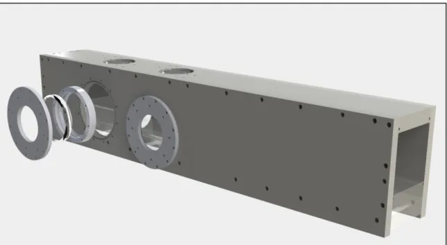
(2012). ... 28 Figure 3.1 Supersonic wind tunnel used in the current study ... 37 Figure 3.2 Contours of the Mach 4.9 nozzle used in the current study. ... 40 Figure 3.3 Test section assembly, with an exploded view of the side window
frame. ... 41 Figure 3.4 Cross-section of the diffuser geometry. ... 42
xi
Page
Figure 3.5 Schematic of diamond roughness topology (Ekoto et al. 2008) ... 47
Figure 3.6 Perspective view of diamond roughness elements ... 48
Figure 3.7 Convex curvature of favorable pressure gradient models. ... 50
Figure 3.8 Surface roughness of smooth-wall models ... 51
Figure 4.1 A schematic of a typical schlieren arrangement, showing the effects of light ray deflection. ... 55
Figure 4.2 “Z-type” schlieren arrangement used in current experiment ... 57
Figure 4.3 Color schlieren filter, used with continuous incandescent light-source. ... 58
Figure 4.4 Sample schlieren photographs, using a color cut-off filter oriented in the wall-normal direction. ... 59
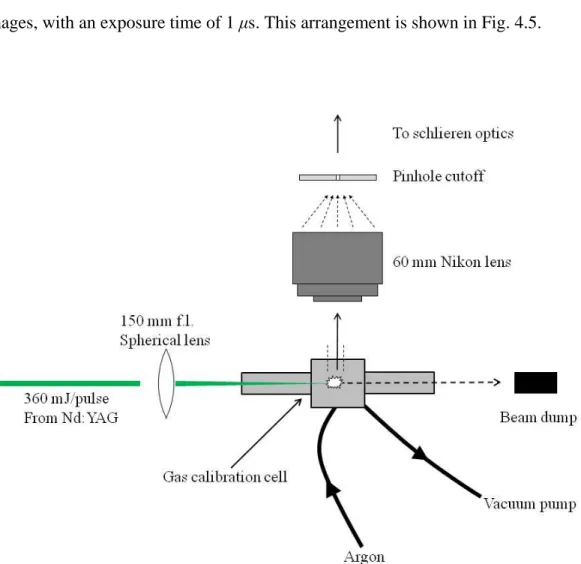
Figure 4.5 Schematic of gas breakdown “spark-source”, for use in schlieren imaging ... 60
Figure 4.6 Sample schlieren images, using a gas breakdown-generated spark source. ... 61
Figure 4.7 Overview of PIV technique, describing the five key steps in data collection and processing ... 63
Figure 4.8 Drawing of PIV experimental arrangement, showing the camera system, laser sheet, and test section. ... 69
Figure 4.9 PIV seeder used in current experiment. ... 71
Figure 4.10 Sample raw image collected over smooth ZPG model, showing instantaneous seed particle concentration. ... 73
Figure 4.11 Waveform of the particle response time τp, compared to a displacement over the timescale Δt. ... 75
xii
Page Figure 4.12 Sketch of quadrants used in quadrant decomposition ... 84 Figure 4.13 Depiction of the integral length scale L11 ... 85 Figure 4.14 Longitudinal auto-correlation of u’ at y/δ = 0.5, for the smooth ZPG
case.. ... 86 Figure 5.1 Vorticity contour of an instantaneous velocity field, for the smooth ZPG
case. ... 91 Figure 5.2 Galilean decomposition of an instantaneous velocity field, after
subtracting a convective velocity Uc = 0.83Ue. ... 92 Figure 5.3 Galilean decomposition of an instantaneous velocity field, after
subtracting a convective velocity Uc = 0.96Ue. ... 93 Figure 5.4 Contours of swirling strength λci, after subtracting a convective velocity
Uc = 0.83Ue. ... 99
Figure 5.5 Contours of swirling strength λci, after subtracting a convective velocity
Uc = 0.96Ue.. ... 100 Figure 5.6 “False positive” vortices detected by the Q-criterion ... 104 Figure 5.7 Comparison of the swirling strength (lines) and Q-criterion (contours). ... 105 Figure 5.8 Comparison of the swirling strength (lines) and corrected Q-criterion
(contours). ... 105 Figure 5.9 PDF of the swirling strength for the smooth ZPG case, scaled by
( )
rm s ci y
at each height. ... 108 Figure 5.10 Templates used for determining the size of a vortex. ... 109 Figure 5.11 Examples of locally spiraling particles traces, showing the effects of r
xiii
Page Figure 5.12 PDF of the inverse spiraling compactness, shown for the smooth ZPG
case. ... 111
Figure 5.13 Examples of synthetic vortices, showing the effects of misalignment with the measurement plane. ... 112
Figure 5.14 PDF of the swirling strength for the smooth WPG case, scaled by ( ) rm s ci y at each height. ... 114
Figure 5.15 PDF of the swirling strength for the smooth SPG case, scaled by ( ) rm s ci y at each height. ... 115
Figure 5.16 PDF of the swirling strength for the rough-wall case, scaled by ( ) rm s ci y at each height. ... 115
Figure 5.17 PDF of the inverse spiraling compactness, shown for the smooth WPG case. ... 116
Figure 5.18 PDF of the inverse spiraling compactness, shown for the smooth SPG case. ... 116
Figure 5.19 PDF of the inverse spiraling compactness, shown for the rough-wall case. ... 117
Figure 6.1 Mean velocity profile. ... 120
Figure 6.2 Inner-scaled mean velocity, using the van Driest II compressibility transformation. ... 121
Figure 6.3 Morkovin-scaled velocity fluctuations ... 122
Figure 6.4 Reynolds shear stress profiles, scaled by wall shear stress τw. ... 123
Figure 6.5 Reynolds shear stress profiles for supersonic studies. ... 124
xiv
Page
Figure 6.7 Normalized spectra of the wall-normal stress component ... 126
Figure 6.8 Normalized shear spectra ... 128
Figure 6.9 Two-point correlations of the u-velocity. ... 130
Figure 6.10 One-dimensional autocorrelation of Ruu, presented at y/δ = 0.5 ... 132
Figure 6.11 Streamwise length scale, plotted versus the Mach 2 DNS of Pirozzoli & Bernardini (2011). ... 133
Figure 6.12 Structure angles of two-point correlations, computed for the current study at Ruu = 0.4. ... 135
Figure 6.13 Instantaneous velocity field for baseline case, showing a hairpin vortex packet. ... 137
Figure 6.14 Instantaneous velocity field of incompressible boundary layer, taken from Adrian et al. (2000). ... 138
Figure 6.15 Schematic of an individual hairpin vortex, describing the sweep and ejection events. ... 139
Figure 6.16 Premultiplied spectra of streamwise velocity component, plotted versus wavelength Λx ... 142
Figure 6.17 Premultiplied spectra of wall-normal velocity component, plotted versus wavelength Λx ... 142
Figure 6.18 Premultiplied shear spectra, plotted versus wavelength Λx ... 143
Figure 6.19 Instantaneous velocity field, showing vortices identified by the swirling strength criterion λci. ... 147
Figure 6.20 a) Streamwise and b) wall-normal convective velocity components, plotted versus the respective mean velocities. ... 148
xv
Page Figure 6.21 Streamwise convective velocity Uc, scaled by the local mean velocity
U, plotted versus outer-scaled coordinates. ... 148
Figure 6.22 Streamwise convective velocity Uc, scaled by the local mean velocity U, plotted versus viscous-scaled coordinates. ... 149
Figure 6.23 Population distribution of vortices, computed as a PDF. ... 152
Figure 6.24 Autocorrelations of prograde swirling strength p ci . ... 155
Figure 6.25 Autocorrelations of retrograde swirling strength r ci . ... 155
Figure 6.26 Cross-correlation of prograde and retrograde swirling strength, indicating the position of retrograde events relative to a reference prograde vortex ... 157
Figure 6.27 Instantaneous velocity field, showing shear layers forming downstream of the vortices. ... 158
Figure 6.28 Conditionally averaged velocity field for prograde vortex event ... 160
Figure 6.29 Conditionally averaged velocity field for retrograde vortex event ... 161
Figure 6.30 Cross-correlation of prograde swirling strength and shear stress ... 163
Figure 6.31 Cross-correlation of retrograde swirling strength and shear stress. ... 164
Figure 6.32 One of several possible merging scenarios for adjacent hairpin vortices, showing the creation of a large prograde vortex and a smaller retrograde vortex (shown in green). Image is adapted from Tomkins & Adrian (2003). ... 166
Figure 6.33 Ratio of streamwise convective velocities, for prograde and retrograde vortices ... 167
Figure 6.34 Conceptual diagram of omega-shaped vortex loop, showing the possible orientation of retrograde and prograde vortices. ... 169
xvi
Page Figure 7.1 Mean streamwise velocity profile. ... 175 Figure 7.2 Mean wall-normal velocity profile ... 175 Figure 7.3 Inner-scaled mean velocity, using the van Driest II compressibility
transformation ... 176 Figure 7.4 Axial kinematic stress over the FPG models, scaled by the freestream
velocity ... 177 Figure 7.5 Wall-normal kinematic stress over the FPG models, scaled by the
freestream velocity ... 178 Figure 7.6 Kinematic shear stress over the FPG models, scaled by the freestream
velocity. ... 178 Figure 7.7 Transformed kinematic shear stress over the FPG models, scaled by the
freestream velocity. ... 180 Figure 7.8 Quadrant decomposition of the FPG boundary layers, showing the
contribution of each quadrant event. ... 181 Figure 7.9 Distribution of quadrant events within each test case ... 183 Figure 7.10 Streamwise evolution of the axial kinematic stress over the SPG model ... 186 Figure 7.11 Streamwise evolution of the wall-normal kinematic stress over the
SPG model ... 187 Figure 7.12 Streamwise evolution of the kinematic shear stress over the SPG
model ... 187 Figure 7.13 Two-point correlations Ruu, computed at locations y/δ ≥ 0.3 ... 190
xvii
Page Figure 7.15 Two-point correlations Ruu, computed at wall-normal locations y/δ =
0.1 (left column) and 0.2 (right column).. ... 192 Figure 7.16 Streamwise length scales ... 193 Figure 7.17 Structure angles of FPG boundary layers, computed from Ruu = 0.4
isocontour. ... 194 Figure 7.18 Structure angles of FPG boundary layers, transformed into wind tunnel
axes. ... 195 Figure 7.19 Major (hollow symbols) and minor (filled symbols) axes for the FPG
boundary layers. ... 196 Figure 7.20 Major (hollow symbols) and minor (filled symbols) axes for the FPG
boundary layers, scaled by the ZPG boundary layer thickness. ... 198 Figure 7.21 Streamwise length scales, estimated from the autocorrelations at Ruu =
1/e, and scaled by the ZPG boundary layer thickness. ... 199 Figure 7.22 Instantaneous velocity field for the SPG boundary layer. ... 201 Figure 7.23 Instantaneous velocity field for the SPG boundary layer, showing the
increased orientation angle of the structures. ... 202 Figure 7.24 Instantaneous velocity field of the SPG boundary layer, showing a
vertical “stack” of vortices. ... 203 Figure 7.25 Premultiplied spectra of the fluctuating u-velocity component, for y/δ
≤ 0.1. Outer scaling is applied to the wavelengths. ... 206 Figure 7.26 Premultiplied spectra of the fluctuating u-velocity component, for y/δ
≤ 0.1. Inner scaling is applied to the wavelengths. ... 207 Figure 7.27 Premultiplied spectra of the fluctuating v-velocity component, for y/δ
xviii
Page Figure 7.28 Premultiplied spectra of the fluctuating v-velocity component, for y/δ
≤ 0.1. Inner scaling is applied to the wavelengths. ... 210 Figure 7.29 Premultiplied spectra of the fluctuating u-velocity component, for y/δ
≥ 0.3. Outer scaling is applied to the wavelengths. ... 211 Figure 7.30 Premultiplied spectra of the fluctuating v-velocity component, for y/δ
≥ 0.3. Outer scaling is applied to the wavelengths. ... 211 Figure 7.31 Premultiplied spectra of the fluctuating u-velocity component,
computed over the upstream and downstream halves of the SPG boundary layer. Outer scaling is applied to the wavelengths. ... 212 Figure 7.32 Streamwise convective velocity Uc, scaled by the local mean velocity ... 214 Figure 7.33 Wall-normal convective velocity Vc, scaled by the local mean velocity .... 216 Figure 7.34 Autocorrelation of the prograde swirling strength, for the ZPG
boundary layer ... 217 Figure 7.35 Autocorrelation of the prograde swirling strength, for the SPG
boundary layer ... 218 Figure 7.36 Vortex population distribution. ... 219 Figure 7.37 Conditional average of the ZPG velocity fields, using a prograde
vortex as the conditional event. ... 222 Figure 7.38 Conditional average of the WPG velocity fields, using a prograde
vortex as the conditional event. ... 223 Figure 7.39 Conditional average of the SPG velocity fields, using a prograde
vortex as the conditional event. ... 224 Figure 7.40 Comparison of the ZPG (left column) and SPG (right column)
conditionally averaged velocity fields, at y/δ = 0.1 (top row) and y/δ = 0.2 (bottom row). ... 225
xix
Page Figure 7.41 Cross-correlation of prograde swirling strength and shear stress, for
the ZPG boundary layer. ... 227 Figure 7.42 Cross-correlation of prograde swirling strength and shear stress, for
the WPG boundary layer. ... 228 Figure 7.43 Cross-correlation of prograde swirling strength and shear stress, for
the SPG boundary layer. ... 229 Figure 7.44 Cross-correlation of prograde swirling strength and shear stress, for
the SPG boundary layer, after rotating the coordinate frame into the wind tunnel axes. ... 231 Figure 7.45 Schematic of a hairpin vortex, identifying the motions contributing to
sweeps and ejections ... 235 Figure 7.46 Illustrations of the possible mechanisms contributing to the reduced
magnitude of the ejection events, including a) vortex spreading and b) reduced vorticity. ... 236 Figure 7.47 Outer-scaled autocorrelation of the u’ velocity component, presented
in the spanwise direction at y/δ = 0.2. Data were provided by English (2013) ... 236 Figure 7.48 Mean prograde swirling strength, non-dimensionalized by the ZPG
boundary layer thickness and freestream velocity ... 238 Figure 7.49 PDF of prograde swirling strength (after filtering for
size/strength/orbital compactness) ... 240 Figure 7.50 Summary of FPG results, showing the relation between the
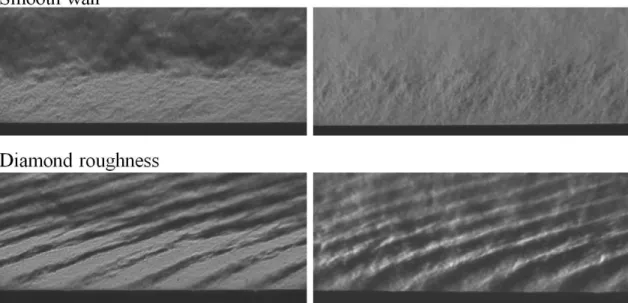
deformation of the turbulent structures and the measured Reynolds shear stress ... 243 Figure 8.1 Schlieren images of smooth-wall (left) and diamond roughness (right)
xx
Page Figure 8.2 Schlieren images of smooth (top row) and diamond roughness (bottom
row) boundary layers, using a short-duration spark-source. ... 246
Figure 8.3 Streamwise velocity profiles of the smooth and rough flowfields. ... 249
Figure 8.4 Inner-scaled streamwise velocity, presented using the van Driest II transformation. ... 249
Figure 8.5 Comparison of the inner-scaled streamwise velocity, extracted from multiple positions over the roughness element. ... 250
Figure 8.6 Positioning of PIV laser sheet over the roughness topology. ... 251
Figure 8.7 Streamwise evolution of rough-wall velocity u/U, plotted versus x/δ. ... 252
Figure 8.8 Streamwise evolution of rough-wall velocity v/U, plotted versus x/δ. ... 253
Figure 8.9 Rough-wall axial stress, extracted from multiple positions over a roughness element. ... 254
Figure 8.10 Rough-wall wall-normal stress, extracted from multiple positions over a roughness element. ... 254
Figure 8.11 Rough-wall shear stress, extracted from multiple positions over a roughness element. ... 255
Figure 8.12 Streamwise evolution of rough-wall shear stress, plotted versus x/δ. ... 256
Figure 8.13 Inner-scaled axial stress. Data are scaled by the respective friction velocities. ... 258
Figure 8.14 Inner-scaled wall-normal stress. Data are scaled by the respective friction velocities. ... 259
Figure 8.15 Inner-scaled shear stress. Data are scaled by the respective friction velocities. ... 259
xxi
Page Figure 8.16 Inner-scaled axial stress. Data are scaled by the smooth-wall friction
velocity. ... 260 Figure 8.17 Inner-scaled wall-normal stress. Data are scaled by the smooth-wall
friction velocity. ... 261 Figure 8.18 Inner-scaled shear stress. Data are scaled by the smooth-wall friction
velocity. ... 261 Figure 8.19 Comparisons of scaling effects upon the axial stress. Left: current
study. Right: Sahoo et al. (2010) ... 262 Figure 8.20 Comparisons of scaling effects upon the wall-normal stress. Left:
current study. Right: Sahoo et al. (2010) ... 263 Figure 8.21 PDFs of the instantaneous shear stress events, scaled by the
smooth-wall friction velocity. ... 264 Figure 8.22 Stress contributions of quadrant events, as determined by quadrant
decomposition. ... 266 Figure 8.23 Two-point correlations of the fluctuating streamwise velocity, Ruu,
plotted in the outer region y/δ ≥ 0.3 ... 268 Figure 8.24 Two-point correlations of the fluctuating streamwise velocity, Ruu,
plotted in the near-wall region. ... 269 Figure 8.25 Major and minor axes of the two-point correlations, determined from
the Ruu = 0.4 isocontour. ... 270
Figure 8.26 Orientation angle of the large-scale motions, determined from the Ruu
= 0.4 isocontour. ... 272 Figure 8.27 Streamwise dependency of major axis of large-scale motions, for
rough-wall boundary layer. ... 274 Figure 8.28 Streamwise dependency of the orientation angle of the large-scale
xxii
Page Figure 8.29 Premultiplied spectra of the fluctuating streamwise velocity,
normalized by the mean axial stress at each height. Spectra are shown for heights y/δ ≤ 0.1. ... 276 Figure 8.30 Premultiplied spectra of the fluctuating streamwise velocity,
normalized by the mean axial stress at each height. Spectra are shown for heights y/δ ≥ 0.3. ... 277 Figure 8.31 Premultiplied spectra of the fluctuating wall-normal velocity,
normalized by the mean transverse stress at each height. Spectra are shown for heights y/δ ≤ 0.1.. ... 278 Figure 8.32 Premultiplied spectra of the fluctuating wall-normal velocity,
normalized by the mean transverse stress at each height. Spectra are shown for heights y/δ ≥ 0.3.. ... 279 Figure 8.33 Streamwise convective velocity, divided by the local mean velocity. ... 280 Figure 8.34 Wall-normal convective velocity, divided by the local mean velocity. ... 281 Figure 8.35 Population distribution of spanwise vortices, as detected by the
swirling strength λci ... 283
Figure 8.36 Comparison of prograde and retrograde vortex populations ... 284 Figure 8.37 Top: Instantaneous realization of rough-wall vector field, showing
steeply angled vortex alignments. Bottom: Portion of rough-wall flowfield examined in top image. ... 285 Figure 8.38 Conditionally averaged velocity field of the rough-wall boundary
layer, based upon the presence of a prograde vortex event. ... 287 Figure 8.39 Mean prograde swirling strength, describing the rotational rate of the
spanwise vortices ... 289 Figure 8.40 Axes of coordinate transformation, described in Eqns. 8.2 – 8.4 ... 291
xxiii
Page Figure 8.41 Transformed axial stress, following the coordinate transformation in
Eqn. 8.2 ... 293 Figure 8.42 Transformed wall-normal stress, following the coordinate
transformation in Eqn. 4.3 ... 293 Figure 8.43 Transformed shear stress, following the coordinate transformation in
Eqn. 8.4 ... 294 Figure 8.44 Ratios of the structure angle and wall-normal stress, where the
rough-wall value is scaled by the associated smooth-rough-wall value at each height. ... 295 Figure 9.1 Isolated roughness element in a supersonic flow, showing the
contributions of surface/viscous and form drag ... 307 Figure A.1 TSP calibration cell, showing CCD camera and LED arrays
(thermocouple and electric heater are not shown) ... 326 Figure A.2 Surface roughness of TSP, measured using a Mitutoyo SJ-400
profilometer. ... 328 Figure A.3 Wall temperature of the baseline model, measured with ISSI UNT
temperature sensitive paint. ... 329 Figure A.4 Wall temperature of the smooth SPG model, measured with ISSI UNT
temperature sensitive paint. ... 330 Figure B.1 Velocity profile, showing the relation between εδ and dU/dy. ... 335
Figure B.2 Mean velocity profile, showing the effect of dU/dy ≈ 1 on the uncertainty εδ.. ... 336 Figure B.3 Mean velocity profile, showing the effect of dU/dy → 0 on the
uncertainty εδ. ... 337 Figure B.4 Calculated particle slip, for rough-wall boundary layer ... 340
xxiv
Page Figure C.1 Comparison of ensemble-averaged shear stress for all cases listed in
Table C.1. ... 346 Figure C.2 Comparison of averaging filters for Case 8 ... 347 Figure D.1 High-pressure seeder. Left: full view, showing critical components and
flowpath. Right: cross-section, showing angled copper tubing ... 349 Figure E.1 Sensitivity of streamwise convective velocity to vortex ID filters. ... 353 Figure E.2 Sensitivity of wall-normal convective velocity to vortex ID filters. ... 353 Figure E.3 Sensitivity of total vortex population to vortex ID filters ... 354 Figure E.4 Sensitivity of prograde vortex population to vortex ID filters ... 355 Figure E.5 Sensitivity of retrograde vortex population to vortex ID filters ... 355 Figure G.1 Streamwise evolution of u-velocity versus x/δ. ... 358 Figure G.2 Streamwise evolution of v-velocity versus x/δ. ... 359
xxv
LIST OF TABLES
Page Table 2.1 Representative sample of available high-speed rough-wall data ... 30 Table 3.1 Nominal tunnel operating conditions ... 44 Table 3.2 Parameters for convex curvature ... 49 Table 4.1 PIV experimental parameters ... 70 Table 4.2 PIV processing and filter settings, used in DaVis 8.0.2 ... 78 Table 4.3 Statistical uncertainty for the baseline flowfield ... 79 Table 6.1 Freestream and wall conditions of the baseline flowfield ... 119 Table 7.1 Mean flow parameters ... 174 Table 8.1 Flow parameters for smooth and rough boundary layers ... 247 Table B.1 Uncertainty parameters of PIV calculations ... 333 Table C.1 Comparison cases, for determining sensitivity of PIV settings ... 345 Table E.1 Vortex ID filter settings ... 352
1
1.INTRODUCTION
1.1. Motivation
On October 14, 1947, Captain Charles “Chuck” Yeager became the first human being to pilot a supersonic aircraft (all previous supersonic craft were unmanned rockets). This groundbreaking feat set the stage for repeated aeronautical discoveries in the second half of the 20th century. While the pace of these discoveries has waxed and waned in phase with public interest and funding availability, the desire to achieve ever-greater speeds has remained. Over sixty years after Capt. Yeager’s historic flight, these same desires motivate the current efforts in developing a hypersonic (Mach > 5) air-breathing vehicle. Potential applications include military (global strike and high-speed interceptors), commercial (fast-response international cargo transportation), and space-launch (reusable first stage) customers.
The stresses, both mechanical and thermal, experienced by a high-Mach number vehicle can prove instrumental in defining the performance envelope of the aircraft. The advanced propulsion systems necessary to accelerate a vehicle to high Mach numbers, which primarily include ramjets and scramjets, have much lower efficiencies than turbofan engines. For example, a hydrocarbon-fueled ramjet operating at Mach 5 will perform at approximately 25% of the efficiency of a subsonic turbojet engine (Fry 2004). It is not uncommon for such vehicles to be designed to operate near the thrust margin. Therefore, it is essential that the stresses acting upon the vehicle be accurately predicted. For a slender-bodied vehicle, such as the X-43 or X-51, the majority of these stresses are due to viscous effects caused by the turbulent boundary layer (TBL) over the vehicle surface. It is this feature that will be the focus of this dissertation.
The mere presence of a high-Mach number turbulent boundary layer does not present a great challenge to the current suite of predictive tools available to aerodynamicists. This is due primarily to the findings of Morkovin (1961), who showed that the behavior of a compressible turbulent boundary layer, up to and including the second-order statistics,
2
can be modeled as an incompressible boundary layer, when the density stratification of the flow is taken into account. However, this notion, labeled succinctly as Morkovin’s hypothesis, is predicated on the stipulation that the flowfield is canonical, i.e. a smooth-wall, flat-plate boundary layer. It is over such surfaces that a majority of the current knowledge on supersonic boundary layers was developed, which will be discussed in §2. In reality, these flowfields are rarely found in practical aeronautical applications. While modeling a vehicle as a collection of flat plates would simplify the efforts needed for predicting the stresses exerted by the turbulent boundary layer, this ignores many key physical phenomena that may adversely (or favorably) affect the performance and survivability of the aircraft.
Figure 1.1 Schematic of a typical hypersonic vehicle, indicating potential areas for mechanical distortions. Image taken from Pratt and Whitney.
Visualizing a prototypical high-Mach number vehicle (Fig. 1.1), several key features become apparent. Every supersonic vehicle (excepting reentry vehicles) utilizes a lifting surface, whether that is a traditional wing, a blended wing-body, or simply a control surface. Regardless the type of surface, the pressure distribution across this area will not be uniform, whether due to boundary layer growth or viscous-inviscid interactions,
3
thereby inducing a pressure gradient within the boundary layer. Pressure gradients also exist in regions near shock boundary layer interactions, and along surface curvature (e.g. cambered airfoils). Given that pressure gradients exist in such mission-critical areas, it is essential to understand the effects of these distortions on the boundary layer, including the distribution of turbulent stresses, which affect both the overall drag and heat transfer rate. Another departure from the canonical smooth-wall, flat-plate boundary layer occurs due to surface roughness. While the majority of the surface area of most aircraft is hydraulically smooth, any aircraft will contain isolated roughness (e.g. rivets, seams, machining imperfections). However, distributed roughness is commonly found on high-Mach number vehicles, leading to large distortions of the boundary layer structure. This prevalence of organized roughness patterns is due to the necessity of thermal protection systems (TPS), owing to the high surface temperatures experienced in flight. Two common forms of TPS are tiled and ablative. In the former configuration, insulating tiles (composed of metallic, ceramic, or carbon/carbon components) are arrayed along the windward surface of the vehicle in a square, diamond, or hexagonal grid. Consequently, the seams between the tiles can manifest themselves within the turbulent boundary layer as periodic roughness. This effect can be amplified by metallic tiles, which may bow outward due to temperature gradients within the TPS material (Berry et al. 1999). Ablative TPS, while initially smooth, may also develop a periodic roughness pattern, due to the naturally occurring phenomenon of cross-hatching. The ablative material is designed to react endothermically, extracting energy that would otherwise be conducted into the vehicle. However, researchers discovered in the 1960s that the surface material receded at a non-uniform rate, producing a diamond pattern of streamwise grooves (Larson & Mateer 1968). This transient process is observed in supersonic TBLs, and was initially believed to be a result of differential ablation caused by heat-transfer perturbations over a wavy surface (Laganelli & Nestler 1969), though later experiments showed that cross-hatching would naturally occur in the surface layer of viscoelastic solids and liquid films [Gold & Probstein 1970; White & Grabow 1973; Stock 1975],
4
absent any ablative mass transfer. Figure 1.2 offers examples of these roughness patterns.
Figure 1.2 Examples of distributed roughness. Top: Cross-hatching of Teflon (White & Grabow 1973). Bottom: Streaklines over bowed metallic tiles (Berry et al. 1999)
1.2. Overview of Mechanically Distorted Supersonic TBLs
The features described above are labeled collectively as mechanical distortions, and their presence within a flowfield can influence key parameters such as shear stress, heat
5
transfer, and boundary layer growth. A detailed understanding of these features remains a necessary prerequisite for the accurate design of the most promising aeronautical applications. Given the difficulties associated with the numerical modeling of these phenomena, there is a strong motivation to experimentally investigate and quantify these effects. In the current study, periodic surface roughness and curvature-induced favorable pressure gradients (FPGs) have been selected for further examination. Adverse pressure gradients (APGs) are also a promising field of study, generating considerable interest due to their association with ramp flows and shock boundary layer interactions. However, these areas have received increasing attention over the past decade. Therefore, APGs will not be included in this study.
In order to establish what technical and scientific challenges lie ahead, it will prove useful to take a brief historical detour, reviewing the studies that have lead to the current state of knowledge concerning mechanically distorted TBLs. The following sub-sections will separately discuss surface roughness and favorable pressure gradient effects within turbulent boundary layers. This should not be considered an exhaustive review, but merely an introduction to the challenges associated with these distortions, as well as describing the central role they occupy in determining the evolution of the boundary layer.
1.2.1.Surface Roughness
A wealth of data exists for incompressible rough-wall boundary layers, summarized by Nikuradse (1933), Perry, Schofield & Joubert (1969), Grass (1971), Perry, Lim & Henbest (1987), Raupach (1991), Jiménez (2004), and Schultz & Flack (2007), among many others. Delving into the salient features of these reviews is beyond the scope of this dissertation. In this sub-section, the discussion will be confined to studies performed within compressible boundary layers, in order to justify the chosen flowfields for this
6
dissertation. General aspects of rough-wall boundary layers, including the effects on classical scaling, will be discussed more thoroughly in §2.
While studies of rough-wall boundary layers in the incompressible regime have been conducted for nearly a century, investigations into the effects of surface roughness within supersonic boundary layers began in the 1950s. Many of these earliest studies, beginning with Liepmann & Goddard (1957) and Goddard (1959), focused upon the response of the compressible skin-friction coefficient, due to its critical importance in the design process. They found that the skin-friction is solely a function of the roughness Reynolds number k+ = kuτ /ν, where k is the roughness height, uτ is the friction velocity, and ν is the fluid viscosity. Additionally, Goddard (1959) also found that the shift in the velocity profile Δ(u/uτ) is a function of k+ only, when the scaling given by Van Driest (1951) is used to account for the density stratification of the compressible boundary layer. These findings are consistent with the incompressible results of Nikuradse (1933). The next 50 years of research into supersonic rough-wall flows continued in this fashion, addressing the effects of roughness height and topology on the skin-friction and mean velocity scaling. These effects are discussed in §2. It was not until the year 2000 that turbulence measurements were added to the growing database of experimental data. Latin & Bowersox (2000) used laser Doppler velocimetry (LDV) and hot-film anemometry to measure the mean velocity and density, kinematic turbulence intensities, mass flux turbulence intensities, and kinematic Reynolds shear stress over sand-grain and two-dimensional machine roughness elements (ks+ = 100 – 570) at Mach 2.9. The mean velocity, when scaled by Van Driest II theory, followed the trends of incompressible rough-wall flows, in agreement with Goddard (1959). Kinematic turbulence statistics of each roughness topology (excepting the two-dimensional plate) showed similar behavior when scaled with outer variables, collapsing onto a single curve. However, turbulence intensities (ρu), (ρv),and (ρw) did not collapse in a similar manner, instead showing a dependence upon ks+. Also, flow visualizations performed using schlieren photography showed that when the roughness elements protruded into
7
the supersonic region of the flow, shock waves and expansions fans were produced that persisted through the boundary layer thickness. Such features are not found in incompressible flows, suggesting that sufficiently large roughness elements in a supersonic boundary layer may behave differently than their low-speed counterparts. Additional analysis of this same data set by Latin & Bowersox (2002) showed that surface roughness increased the size of the small-scale structures, and decreased the size of the large-scale structures, as inferred from the autocorrelation curves. Using cross-correlations traces, the average structure orientation was unchanged by the sand-grain roughness, while the two-dimensional roughness indicated a lower angle in the outer region of the boundary layer.
Ekoto et al. (2009) used PIV to measure the kinematic turbulence stresses and strain rates over square and diamond roughness at Mach 2.87. Similar to Latin & Bowersox (2000), schlieren photography showed that shock waves and expansions fans were generated by the diamond roughness elements, extending into the outer region of the boundary layer. The elongated nature of the diamond elements resulted in attached waves that were strong enough to induce periodic oscillations in the strain rates and Reynolds shear stress. Measurements using pressure sensitive paint (PSP) showed that these waves generated locally adverse and favorable pressure gradients, corresponding to the attached shock waves and expansion fans, respectively. The stabilizing influence of the local FPG resulted in negative turbulence production over the aft half of each diamond element. The resulting Reynolds shear stress, when averaged over the entire diamond element length, was only 30% larger than the smooth-wall value. Conversely, the square elements increased the Reynolds shear stress by approximately 140%, and exhibited minimal local variations. Measurements of the kinematic stresses, with Morkovin scaling, “for the smooth and square models collapsed onto the expected trend” (Ekoto et al. 2009); the diamond roughness did not scale in a similar manner.
The most recent investigation into high-Mach number rough-wall flows was conducted by Sahoo, Papageorge & Smits (2010), using PIV to interrogate the flow over diamond
8
mesh and square bar elements. The mean velocity showed similar behavior to the incompressible case when scaled with van Driest II theory, again confirming the findings of Goddard (1959). Scaling the turbulence stresses by the local density ratio (ρ/ρw)1/2 did not successfully collapse the data onto a single curve. The scaled rough-wall stresses are
lower than the smooth-wall values, which is in disagreement with the data of Latin & Bowersox (2000). It should be noted that the study by Sahoo et al. (2010) was conducted at Mach 7.3, which is a significantly higher Mach number than that studied by Latin & Bowersox (2000) and Ekoto et al. (2009). This suggests a possible compressibility effect.
These studies, while limited in number, strongly suggest that van Driest II scaling is appropriate for transforming the mean velocity, as per the findings of Goddard (1959). However, Morkovin scaling has shown limited success in supersonic rough-wall boundary layers. The applicability of this scaling appears to be confined to sand-grain roughness (Latin & Bowersox 2000) and square elements (Ekoto et al. 2009), showing good agreement in these cases. For roughness topologies that create persistent distortions through the boundary layer (i.e. shock waves and expansion fans), Morkovin scaling is unsuccessful in collapsing the data. The results of Ekoto et al. (2009) suggest that localized variations in the strain-rates may be responsible, though this has not been confirmed in other studies. Additionally, no explanation is available for the reduced
stresses observed by Sahoo et al. (2010). Further investigations into the local flowfield near roughness-induced distortions may prove fruitful in explaining these behaviors.
1.2.2.Curvature-Driven Favorable Pressure Gradients (FPGs)
The prevalence of curvature-driven FPGs on high-speed vehicles has directly motivated the increased research activity in this area over the last 40 years. Following the format given in the previous sub-section, only the most recent studies into supersonic FPGs will be described here. A more thorough discussion of the fundamental fluid response,
9
including the effects on classical scaling, will be included in §2. The experiments described in the following paragraphs are included to illustrate the importance of this flow phenomenon, and justify its inclusion into the current study.
It has been shown by many researchers that favorable pressure gradients exert a stabilizing influence upon the turbulent boundary layer Bradshaw (1974); Dussauge & Gaviglio (1987); Smith & Smits (1991); Smith & Smits (1994); Arnette, Samimy & Elliott (1998)), possibly reverting the flow to a quasi-laminar state if the gradient is of sufficient strength and duration [Narasimha & Sreenivasan (1973)]. Bradshaw (1974) noted that the effect of the FPG upon the turbulence stresses is approximately an order of magnitude larger than predicted by the Reynolds stress transport equation. Using Rapid Distortion Theory (RDT), Smith & Smits (1991) and Dussauge & Gaviglio (1987) found that a majority of the Reynolds stress evolution can be attributed to the role of bulk dilatation.
Velocimetry measurements by Luker, Bowersox & Buter (2000) in a Mach 2.9 curvature-driven FPG boundary layer extended the earlier experimental results, by examining both the turbulence stresses and strain rates. The pressure gradient produced by the curved-wall model was classified as “strong”, based upon Bradshaw’s (1974) distortion parameter d, defined as the ratio of the largest ‘extra strain rate’ over the
primary strain rate dU/dy. The FPG produced reductions in the near-wall axial and shear stresses of 70% and 75%, respectively. In the outer region, u’v’ experienced a sign reversal, indicating negative turbulence production in this area of the boundary layer. Additionally, measurements at the boundary layer edge suggested an increase in intermittency.
Ekoto et al. (2009) employed PIV to interrogate the boundary layer response over two gradual expansions, d ≈ 0.1 and d ≈ 0.3 – 0.4, at Mach 2.87. These models, labeled as ‘weak’ and ‘strong’ pressure gradients, reduced the near-wall shear stress by 20% and 40%, respectively. The largest ‘extra’ strain rate was dV/dy, due to the expansion of the boundary layer, leading to a significant change in the bulk dilatation for the strong FPG
10
case. The bulk dilatation for this case was approximately 30% - 50% of the principal strain rate. The axial normal stress production was negative at y/δ = 0.4, indicating that energy is flowing from the turbulent fluctuations into the mean flow.
The most recent study into supersonic curvature-driven FPGs was conducted at Mach 4.9 by Tichenor, Humble & Bowersox (2013). Using the same smooth-wall experimental models as Ekoto et al. (2009), they investigated the coupling between the strain-rates and kinematic stresses, finding that the observed sign reversal of the shear stress occurred where the dilatation was larger than the xy-strain. It was shown that the Reynolds stress transport models, specifically the model proposed by Launder, Reece & Rodi (1975), naturally capture the observed trends in the Reynolds shear stress. Additionally, the statistical size of the large-scale structures was estimated using two-point correlations of the fluctuating velocity, finding that the structures decreased in size through the expansion.
The studies described above confirm the expected trend in FPG boundary layers, showing reduced shear and normal stresses. These trends appear to be driven by the response of the strain rates, including the relative magnitudes of the dilatation and xy-strain. It has been suggested (Luker et al. 2000) and shown [Tichenor et al. (2013)] that the boundary layer structures are reduced in size by the FPG, potentially increasing the amount of energy available for dissipation, and thus contributing to the overall stabilization of the flow. However, RDT analyses by Smith & Smits (1991) and Dussauge & Gaviglio (1987) showed that bulk dilatation is the primary contributor to the response of the boundary layer. Intuitively, it is expected that the turbulent structures would expand with the mean flow, instead of decreasing in scale. To date, no mechanism has been found to explain the disintegration or contraction of the turbulent structures within a favorable pressure gradient. This necessitates a detailed investigation into the response of the boundary layer structures through an expanding flow, focusing upon the deformation of the turbulent eddies.
11
1.3. Research Framework
As shown above, the current knowledge of supersonic distorted TBLs relies almost exclusively upon a limited set of experimental data. While these studies have been instrumental in establishing the effects of mechanical distortions upon the boundary layer structure, a commonality between these analyses is apparent, namely the reliance upon statistical measurements, e.g. turbulent stresses u’u’ and u’v’. This provides useful data concerning the Reynolds stress response of the fluid, which supports the ultimate goal of predicting the stresses produced by a distorted TBL. However, two questions remain unanswered by these measurements: “why” and “how”. Specifically, why do the turbulent stresses exhibit the measured trends, and how do the distortions interact with the fluid to produce these trends?
A turbulent boundary layer is composed of organized structures (described more thoroughly in §2), ranging in size from the boundary layer thickness δ to the Kolmogorov scale η, whose coherent motions comprise a majority of the turbulent stresses generated within the boundary layer (Adrian, Meinhart & Tomkins 2000). The boundary conditions of the flowfield (e.g. mechanical distortions) are introduced through the large-scale structures. As energy is transferred to successively smaller scales through the energy cascade (Richardson 1922), the influence of these distortions will spread beyond the initial large eddies, affecting both the scale and energy content of the resultant structures. It is through this mechanism that mechanical distortions affect the turbulent kinetic energy (TKE), and therefore the turbulent stresses.
From the studies described in the previous section, it is clear that researchers have attempted to use the measured statistics to infer the effects of mechanical distortions upon the turbulent structures. Single-point measurements, including those produced by spatially averaging two-dimensional data, “are ideal for determining the statistical properties of turbulence, [but] are much less satisfactory for revealing the existence of organized flow structures” (Head & Bandyopadhyay 1981). In order to determine how these distortions produce the observed changes in the turbulent stresses, it is necessary to
12
visualize the behavior of the instantaneous eddies under both undistorted and distorted conditions. Unfortunately, resolving the structures responsible for the production and redistribution of TKE is technically challenging, owing to the small scales responsible for these processes.
The rationale for the current study is inspired by the argument of Clauser (1956), who in turn invoked the analogy given by Maxwell, which is adapted here for the current study. Any complex system may be simplified as a self-contained mechanism, whose output is determined solely by external influences. This “black box” analogy essentially states that by varying the input to this system, and observing the output, the inner workings of the system may be deduced. To illustrate this point, Clauser (1956) suggested that any system can be imagined as a “complicated machine”, contained within a windowless room. The machine is controlled by a series of levers, and the output is presented as a collection of lights. The internal workings of the machine are unknown to the operator. If the levers are actuated in a systematic manner, and if the colors of the lights are correlated with the positions of the levers, then it is possible for the operator to deduce the inner workings of this machine. While this approach may seem simplistic, it is commonly used throughout our daily lives. For example, it is trivial to draw a crude circuit diagram of a light switch, simply by flipping the switch and observing the result. No knowledge of electrical engineering is necessary.
13
Figure 1.3 Cartoon describing “black box” analysis method for a turbulent boundary layer
This same “black box” analysis has been used to study mechanical distortions in supersonic TBLs (see Fig. 1.3). Surface curvature, roughness topology, and pressure gradients are the “input”, and the measured turbulence statistics are the “outputs.” By changing the surface orientation or the roughness height, and observing the change in turbulence statistics, researchers have attempted to discern the response of the turbulent eddies within the boundary layer. For example, Luker et al. (2000) suggested that the measured reduction in shear stress u’v’, coupled with the increase in intermittency, indicated that FPGs are responsible for breaking up the large-scale eddies, though no visualization of these structures was obtained. This approach to scientific research can be very successful, and is commonly used in many disciplines. However, there is a potential
14
weakness with this approach, not with the analyses per se, but with the application of the conclusions.
Referring back to the motivation described in §1.1, the objective of this study is to provide insight into the fluid dynamics governing high-Mach number distorted TBLs, supporting the ultimate goal of predicting the flowfield over a supersonic vehicle. Practically, this requires the development and refinement of predictive turbulence models. Using the “black box” analysis described above, model developers are only given the time-averaged turbulence statistics. This necessitates a trial-and-error
approach, adjusting the model constants to produce the desired result. The added disadvantage is that the resulting model is now narrowly optimized for the given conditions and geometries. This laborious approach could be mitigated if researchers were aware of what processes produced the observed results, which could guide the developers in refining the model. For example, instead of attempting to match the reduced shear stress produced by a FPG, turbulence modelers would also know that the observed stress levels are caused by a near-cessation of turbulence production within the logarithmic region. Revisiting the light switch analogy described previously, the scientific framework advocated in this study is akin to asking someone with no electrical engineering knowledge to create a model describing a complicated circuit, based only upon observation of the inputs and outputs of the circuit (i.e. “black box” analysis), and then providing that person with a list of the pertinent components and their functions (e.g. capacitors, inductors, batteries). In essence, the current study attempts to remove the lid from the “black box.”
1.4. Scientific Approach
The goal of the current study is to experimentally determine the principal processes governing the behavior of a high-Mach number, mechanically distorted TBL. This is performed by measuring the two-dimensional velocity field within the boundary layer,
15
focusing upon the distribution and deformation of the turbulent structures. High-resolution particle image velocimetry (PIV) is the primary diagnostic used in this study. All experiments are performed at Mach 5, such that the effects of density stratification can be included in the study, while avoiding the thermal non-equilibrium and rarified gas effects associated with the hypersonic regime. The three flowfields under investigation are1:
1) periodic surface roughness
2) curvature-driven favorable pressure gradients 3) a flat-plate, smooth-wall TBL
Details of the three geometries selected above will be described further in §3.2. The final case of an undistorted TBL is included not only for comparing to a baseline flowfield, but to lend insight into the behavior of highly compressible TBLs, motivated by the dearth of experimental data at high Mach numbers. This lack of data is due to the difficulty of resolving the velocity field within the high-shear near-wall region. The low density encountered in this region of compressible boundary layers is a direct obstacle to particle-based velocimetry methods (see §4.2). In general, the seeding density is proportional to the fluid density. Hence, the near-wall region, which is the most active region in turbulence production, and is therefore of greatest interest to the scientific community, also suffers greatly from low signal-to-noise levels. The current study addresses this issue through careful implementation of the PIV diagnostic, including the design and construction of a high-flow seeder (Appendix D), as well as minimization of noise generated by laser reflection (see §4.2). The resulting data sets not only support turbulence model development (as described in the previous section), but also aid in the validation of higher-order simulations (e.g. LES and DES).
Using this high-resolution data, the objective of the current study is to extend the existing knowledge of Mach 5 TBLs, under both distorted and undistorted conditions, by
1
In the current study, the mechanical distortions are studied separately. Data have been collected for the case of rough-wall convex curvature models, but any investigation in the non-linear interaction of these distortions will not be included in this dissertation.
16
examining the response of the turbulent structures. The application of advanced post-processing algorithms allows for the population, distribution, orientation, and intensity of these structures to be directly computed from the experimental data (see §5 for a complete description of the analysis techniques). With this insight, coupled with “traditional” measurements of turbulence statistics, this study will answer the following:
1) How do mechanical distortions modify the turbulent structures in a Mach 5 turbulent boundary layer?
2) How does the modification of these structures manifest itself in the turbulence statistics?
The dissertation is laid out in the following manner. In §2, the fundamentals of turbulent boundary layers, including scaling and compressibility effects, are discussed. This section also includes an overview of pertinent studies of turbulent structures, and introduces key concepts used throughout the discussion of the results. Section 3 describes the wind tunnel facility used in this study, along with the experimental models. Experimental diagnostics are described in §4, and vortex identification techniques are discussed in §5. Results from the baseline undistorted TBL are given in §6, and FPG and rough-wall results are discussed in §7 and §8, respectively. Finally, key conclusions from each of the three flowfields are summarized in §9. This final section also includes recommendations for future analyses of the current results, as well as potential experiments to complement these data sets.
17
2.BACKGROUND REVIEW
The following section provides an overview of the key studies that have contributed to the current understanding of distorted turbulent boundary layers. Unless otherwise noted, the review will focus primarily upon the behavior of compressible boundary layers, and their response to favorable pressure gradients and surface roughness.
2.1. Turbulent Boundary Layer Fundamentals
2.1.1.Coherent Structures in Turbulent Boundary Layers
The dynamics of turbulent boundary layer structures has been the subject of countless studies over the past half-century. As such, this summary is not intended to be an exhaustive review of turbulent structures [for an excellent overview of coherent structures in turbulent boundary layers, see Cantwell (1981); Robinson (1991); Panton (2001); Adrian (2007); Adrian & Marusic (2012) and others]. Instead, the following sections will briefly review the turbulent structure taxonomy, and the contributions of each element to the cycle of Reynolds shear stress production. The technical challenge of experimentally probing highly-compressible boundary layers has largely limited this overview to incompressible boundary layers.
During the earliest years of boundary layer research, turbulence was generally regarded as a purely stochastic process, which could be described by random fluctuations u’ imposed upon a mean flow U [Reynolds (1895)]. While coherent structures and vortices were known to exist, these were regarded as merely passive actors, and were not considered to be a primary component in the production of Reynolds shear stress. However, this paradigm slowly began to evolve in the mid-20th century, originating with the hairpin vortex model proposed by Theodorsen (1952). He suggested that the turbulent fluctuations, and primarily the generation of Reynolds shear stress, within a sheared flow may stem from the passage of an inclined vortex loop, which has been described as a “horseshoe vortex.” The origin of this horseshoe vortex structure was
18
attributed to the wall-normal perturbation of a spanwise vortex filament, causing a segment of the vortex to be momentarily lifted away from the wall. Using a purely kinematic argument, it was suggested that the higher mean velocity experienced by the vortex “head” would stretch the structure in the streamwise direction, while the remnants of the vortex filament within the lower parts of the boundary layer (referred to as the “legs”) would be drawn toward each other. With continued stretching, the initially spanwise-oriented vortex would resemble a horseshoe or hairpin. It was believed that the rotating fluid within the vortices would induce a local flowfield of anti-correlated u’ and
v’ fluctuations, hence producing Reynolds shear stress (see Fig. 2.1). Due to the sense of rotation, the hairpin vortex would “eject” low-momentum fluid away from the wall, while drawing in high-momentum fluid from higher in the boundary layer, a behavior which was later integral to explaining the bursting process observed by Kline et al.
(1967).
The significance of the hairpin vortex model can not be overstated, as it provided a framework by which the seemingly random behavior of the turbulent boundary layer could be described as the result of quasi-deterministic vortex loops. Initially, the implication of these coherent vortex structures was not immediately embraced by the scientific community. In comparison to the early view of a turbulent boundary layer as a chaotic collection of fluctuating velocities, the notion of these macroscopic effects being the manifestation of organized structures was quite unexpected. This reaction was summarized well by Head & Bandyopadhyay (1981):
“At the outset, nothing could have seemed more implausible than that the boundary layer should consist almost exclusively of vortex loops or hairpins originating in the wall region, with dimensions here scaling on wall variables, and that some at least of these same vortex loops or hairpins should extend right through the boundary layer even at high Reynolds numbers (Reθ ≈ 10000), but this is the conclusion we have now come to accept.”