John Murphy
Submitted for the Degree of Ph.D.
Department of Aerospace Sciences Cranfield University
Cranfield, UK
PhD Thesis
John Murphy
December 2008
Cranfield University
School of Engineering
Academic Year: 2008-2009
Supervisor: Dr. David MacManus
c
Cranfield University, 2008.
All rights reserved. No part of this publication may be reproduced without the written permission of the copyright holder.
When an aircraft is operating in static or near static conditions during taxiing or take-off a vortex can form between the ground and the intake. With engine diameters increas-ing, intakes are moving non-dimensionally closer to the ground and as a consequence the likelihood of vortex formation during the aircraft operating envelope is set to in-crease. To date there is little quantitative knowledge therefore a greater understanding is required. This research is aimed at providing an extensive quantitative parametric study of vortex formation leading to advanced design rules for future engines.
A 1/30th scale generic model intake was operated in the Cranfield University 8′× 6′ wind tunnel to examine ground vortex formation under quiescent, headwind and cross-wind conditions. Stereoscopic Particle Image Velocimetry and total pressure measure-ments have been extensively taken to assess the external and internal flowfields. For the first time experiments with a rolling ground plane have been performed to provide insight into the formation and characteristics of ground vortices during take-off. As the velocity ratio reduces a characteristic trend is established whereby the vortex is initially weak, increases in strength to a local maximum and reduces to zero thereafter. The operating points that generate the strongest vortex for a given configuration have been determined and an empirical model has been developed which can predict the vor-tex strength and fan face distortion for any configuration. Under headwind conditions a new vortex formation criterion has been established which also includes contours of vortex circulation. An a priori prediction of the vortex strength under headwind con-ditions has also been developed which considers the approaching and intake induced vorticity sources, the latter of which is determined empirically. Good agreement is found between the model and the experimental dataset. The rolling ground plane ex-periments demonstrate significant sensitivities illustrating that the correct conditions must be simulated properly.
Firstly I would like to thank my supervisor, Dr David MacManus for his endless sup-port, encouragement and direction and in particular for the many hours that he took out of his time to enable me to take the data that is so vital to this thesis. Many thanks must go to Rolls-Royce for their financial and technical assistance and in particular to Chris Sheaf of Installations and JeffGreen of Fan Systems. Thanks to John Thrower of Cranfield University and all the wind tunnel technicians. I would also like to thank Stefan Zantopp and Lauren Rehby for their assistance and discussions.
Thanks to all friends that I have spent my time with at Cranfield University. Special thanks to Ross Chaplin, Peter Thomas, David Estruch, Ben Thornber, Marco Hahn, Macro Kalweit, Sanjay Patel, Sunil Minstry and all those who I have shared the office with over the past three years.
Finally this would not have been possible without the loving support and encourage-ment of my whole family. Much appreciation goes to my Mum, Dad and sister, Kate. I would like to dedicate this thesis to all of my family and in particular to my grand-parents. Without their support, this would have never been possible.
Abstract iii
Acknowledgements v
Nomenclature xxvii
1 Introduction 1
1.1 Current Knowledge . . . 2
1.2 Project Aims and Objectives . . . 3
2 Literature Review 5 2.1 Criteria for Vortex Formation . . . 5
2.2 Mechanisms of Ground Vortex Formation . . . 9
2.2.1 Headwind Mechanism . . . 9
2.2.2 Crosswind Mechanism . . . 17
2.3 Vortex Formation under Tailwind and Reverse Thrust Operation . . . 24
2.4 CFD Studies . . . 27
2.5 Flow Control Methods . . . 28
2.6 Summary . . . 29
2.6.1 Current Knowledge . . . 29
2.6.2 Deficiencies in Current Understanding . . . 30
3 Experiment Approach and Methodology 33 3.1 Experiment Variables . . . 33
3.1.1 Dimensional Analysis . . . 33
3.1.2 Non-dimensional Vortex Strength . . . 34
3.1.3 Reynolds Number . . . 34
3.1.5 Velocity Ratio . . . 35
3.1.6 Yaw Angle . . . 35
3.1.7 Intake Mach Number . . . 35
3.1.8 Approaching Boundary Layer Thickness . . . 36
3.2 Intake Model . . . 36
3.2.1 Intake Suction System . . . 36
3.3 The 8′×6′ Wind Tunnel . . . . 38
3.3.1 Tunnel Configurations . . . 40
3.4 Measurement Techniques . . . 40
3.4.1 Stereoscopic Particle Image Velocimetry . . . 41
3.4.2 Total Pressure Measurement System . . . 45
3.5 Test Matrix . . . 46
3.6 Vortex Characteristics Determination . . . 47
3.6.1 Velocity Measurements . . . 47
3.6.2 Total Pressure Measurements . . . 48
3.7 Uncertainty Analysis . . . 49 3.8 Summary . . . 49 4 Quiescent Conditions 51 4.1 Flow Topology . . . 51 4.1.1 Unsteady Behaviour . . . 52 4.1.2 Flow Modes . . . 55
4.1.3 Vortex Characteristics Quantification . . . 58
4.2 Effect of Non-dimensional Parameters . . . 62
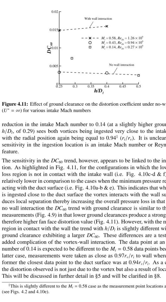
4.2.1 Ground Clearance . . . 62
4.2.2 Intake Mach Number and Reynolds Number . . . 64
4.3 Summary . . . 68
5 Headwind Conditions 71 5.1 Flow Topology . . . 71
5.1.1 In-duct Total Pressure Patterns . . . 77
5.1.2 Snapshot Variations . . . 79
5.2 Effect of Principal Parameters . . . 81
5.2.2 Ground Clearance . . . 85
5.2.3 Approaching Boundary Layer . . . 87
5.3 Vortex Formation Regions . . . 91
5.4 Aerodynamic Self-Similarity . . . 93 5.5 Summary . . . 95 6 Take-offSimulations 97 6.1 Experiment Method . . . 97 6.1.1 Test Configurations . . . 98 6.1.2 Experiment Uncertainties . . . 101
6.2 Synchronized Wind and Road Velocity Experiments . . . 102
6.2.1 PIV Velocity Flowfield Quantification . . . 102
6.2.2 In-duct Total Pressure Survey . . . 110
6.3 Unsynchronized Wind and Road Experiments . . . 112
6.3.1 PIV Velocity Flowfield Quantification . . . 112
6.3.2 Effect of Asynchronous Rolling Road on Vortex Strength . . . 115
6.3.3 Fan face Total Pressure Survey . . . 116
6.4 Further Discussion . . . 117
6.4.1 Implications to Aircraft Operations . . . 119
6.5 Summary . . . 119
7 Crosswind Conditions 123 7.1 Flow Topology . . . 123
7.1.1 Vortex Start-Up Transient . . . 131
7.2 Effect of Principle Parameters . . . 136
7.2.1 Effect of Contraction Ratio . . . 136
7.2.2 Effect of Ground Clearance . . . 142
7.2.3 Approaching Boundary Layer Thickness . . . 146
7.2.4 Effect of Yaw Angle . . . 147
7.3 Further Discussion . . . 152
7.4 Summary . . . 154
8 Discussion and Synthesis 157 8.1 Empirical Model . . . 159
8.1.1 Headwind Vortex Strength Empirical Model . . . 159
8.1.2 Headwind Vortex Distortion Empirical Model . . . 162
8.1.3 Extension to Crosswind . . . 164 8.1.4 Example Application . . . 168 8.2 Theoretical Model . . . 173 8.2.1 Vorticity Sources . . . 173 8.2.2 Estimatation ofΓid . . . 175 8.2.3 Calculation ofΓ∞ . . . 178 8.2.4 Model Results . . . 184 8.3 Further Discussion . . . 194 8.3.1 CFD Studies . . . 194 8.4 Summary . . . 199 9 Conclusions 201 9.1 Quiescent Conditions . . . 201 9.2 Headwind Conditions . . . 202 9.3 Take-offSimulations . . . 202 9.4 Model Development . . . 203 9.5 Crosswind Mechanism . . . 203
9.6 Implications on Model Scale Tests . . . 204
9.7 Applicability of Research to Full Scale Engines . . . 205
9.7.1 Reynolds Number Effects . . . 205
9.7.2 Compressibility Effects . . . 205
9.7.3 Geometric Effects . . . 206
9.8 Implications on Engine Testing and Design . . . 206
9.8.1 Test Bed Experiments . . . 206
9.8.2 Engine Installations . . . 207
9.9 Recommendations for Future Work . . . 208
9.9.1 Further Experimental Investigations . . . 208
9.9.2 Further Model Development . . . 208
A Full Scale Engine Visualizations A-1
A.1 No Wind . . . A-1 A.2 Head Wind . . . A-3 A.3 Cross Wind . . . A-4 A.4 Reverse Thrust . . . A-10
B Experiment Set-Up B-13
B.1 Suction System . . . B-13 B.1.1 Sonic Nozzle Design . . . B-15 B.2 SPIV Set-Up . . . B-16 B.2.1 Optics Configuration . . . B-18
C Empty Wind Tunnel Measurements C-21
C.1 Boundary Layer Measurements . . . C-21 C.2 PIV Measurements of Freestream . . . C-28
D Test Matrix D-33
D.1 Headwind . . . D-33 D.2 Rolling Road Experiments . . . D-36 D.3 Crosswind . . . D-37
E Vortex Characteristics Determination E-39
E.1 Detailed Outline . . . E-39 E.2 Disk Size Determination . . . E-45 E.3 Effect of Disk Resolution . . . E-46 E.4 Method Limitations . . . E-47 E.5 Outlier Detection . . . E-49 E.6 Summary . . . E-50
F Distortion Descriptors F-53
F.1 Loss Coefficient . . . F-53 F.2 The DC60 Parameter . . . F-53 F.3 The KD2Index . . . F-54 F.4 Intensity . . . F-55 F.5 Summary . . . F-57
G Uncertainty Analysis G-61
G.1 Intake Ground Clearance . . . G-61 G.1.1 Error Sources . . . G-62 G.2 Pressure System and Associated Measurements . . . G-63 G.2.1 Determination of Tunnel Speed . . . G-63 G.2.2 Determination of Intake Velocity . . . G-68 G.3 PIV Velocity Error . . . G-74 G.3.1 Bias Errors . . . G-74 G.3.2 RMS Errors . . . G-75 G.3.3 Uncertainty Estimation . . . G-78 G.4 Summary . . . G-80
0.1 Intake Coordinate System . . . xxx 0.2 Definition of intake yaw angle . . . xxxi 1.1 Visualization of an ingested ground vortex on a Rolls-Royce
RB211-524G . . . 1 1.2 Velocity ratio against non-dimensional revealing a region of vortex
for-mation . . . 3 2.1 Illustration of sucked streamtube of an intake far from the ground . . . 6 2.2 Schematic of the sucked streamtube interaction with the ground plane 6 2.3 Correlation of velocity ratio and non-dimensional height combinations
revealing a region of vortex formation and no-vortex formation . . . . 7 2.4 Velocity profiles used in de Siervi et al experiments . . . 10 2.5 Deformation of the ambient vortex lines as they approach the intake
under headwind conditions . . . 11 2.6 Vortex formation under quiescent conditions . . . 13 2.7 Flow modes under headwind conditions . . . 14 2.8 Flow topology observed by Bissenger and Braun under headwind
con-ditions . . . 15 2.9 Formation of the intake vortex system for a twin inlet configuration as
observed by Bissenger and Braun . . . 16 2.10 Flowfield topology under crosswind conditions . . . 17 2.11 Plan view of flowfield under crosswind conditions with a ground
vor-tex showing the separation line over the intake surface . . . 18 2.12 Side view showing the flowfield topology under crosswind conditions
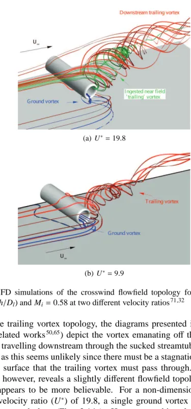
with and without the sucked streamtube interacting with the ground plane . . . 19 2.13 Flow topology for a twin inlet configuration . . . 20 2.14 CFD simulations of the crosswind flowfield topology . . . 21
2.15 Effect of ground clearance and velocity ratio on the non-dimensional vortex strength under crosswind conditions as observed by Shin et al . 23 2.16 Reverse thrust operation introducing an effective tailwind to the intake 24 2.17 Ground vortex ingestion under reverse thrust operation . . . 24 2.18 Effect of wind direction and strength on the vortex location on the
ground plane and its consequent ingestion location . . . 25 2.19 Reverser targeting pattern configurations investigated by Motycka . . 26 2.20 Schematic of two different concepts that have been invented for ground
vortex prevention . . . 28 3.1 Schematic of model dimensions and a picture of the intake illustrating
the total pressure rakes installed . . . 37 3.2 Tunnel configurations for headwind, crosswind and rolling road
exper-iments . . . 39 3.3 Example application of SPIV to the ground vortex flowfield . . . 42 3.4 Measurement planes used in the experiments . . . 44 3.5 Total pressure measurement coverage within the intake for headwind
and crosswind configurations . . . 45 3.6 Primary data points investigated for both headwind and crosswind
con-figurations . . . 46 4.1 Example snapshot of the flowfield under quiescent conditions at the
PIV plane . . . 52 4.2 Example total pressure contour plot under quiescent conditions for the
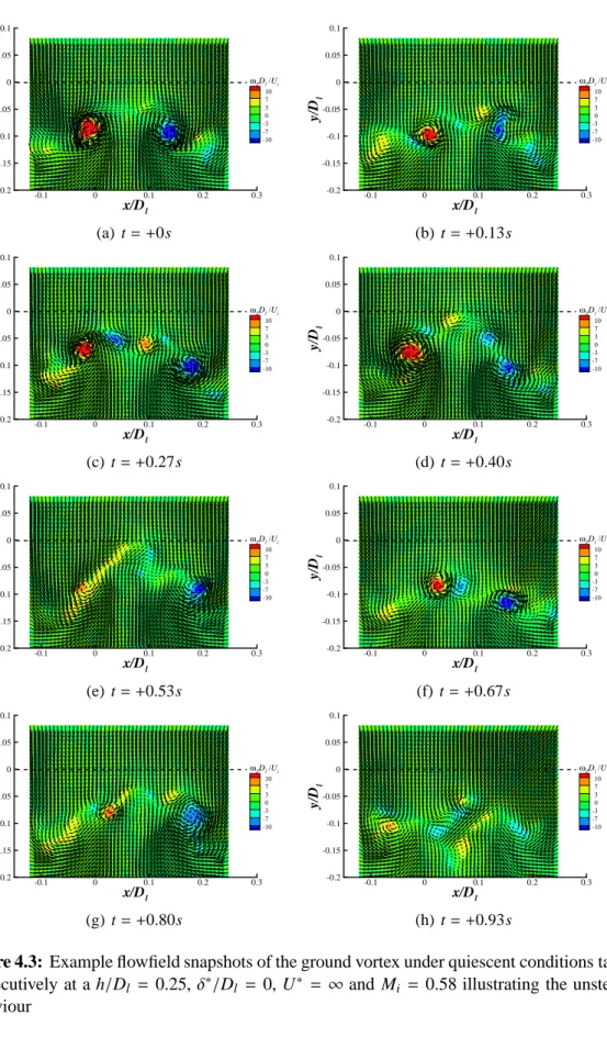
datum height also illustrating the measurement point locations, the PIV plane location and the intake height definition . . . 53 4.3 Example flowfield snapshots of the ground vortex under quiescent
con-ditions taken consecutively illustrating the unsteady behaviour . . . . 54 4.4 Vortex formation under quiescent conditions showing the induced
vor-tex lines approaching the intake in both the positive and negative y directions . . . 55 4.5 Time average flow-field for increasing ground clearance under
quies-cent conditions with corresponding locus of vortex core positions . . . 56 4.6 Flow modes observed under quiescent conditions . . . 57 4.7 Typical variations in the positive vortex strength, core size and Vatistas
vortex model constant . . . 59 4.8 Variation in the vortex circulation under quiescent conditions for the
4.9 Effect of ground clearance on the average non-dimensional vortex strength under no-wind conditions . . . 63 4.10 Effect of ground clearance and intake Mach number on the total
pres-sure contours within the intake duct under quiescent conditions . . . . 65 4.11 Effect of ground clearance on the distortion coefficient under no-wind
conditions . . . 66 5.1 Typical vortex snapshots showing the effect of velocity ratio on the
flowfield topology under headwind conditions . . . 72 5.2 Effect of velocity ratio on the vortex core positions over all flowfield
snapshots under headwind conditions for the datum height configuration 73 5.3 Example headwind flowfield snapshot . . . 74 5.4 Example snapshots under headwind conditions for different non-dimensional
heights and velocity ratios . . . 75 5.5 Flowfield topology under headwind conditions . . . 76 5.6 Fan face total pressure contours under quiescent and headwind
condi-tions . . . 78 5.7 Variations in the vortex strength and core size for headwind conditions 79 5.8 Typical variation of the Vatistas vortex model constant and variation in
the swirl velocity against radial distance from the centre of the vortex for a single headwind snapshot . . . 80 5.9 Total average non-dimensional vortex strength against velocity ratio
under headwind conditions for the datum height configuration . . . . 81 5.10 Effect of increasing headwind speed in the total pressure contours at
the fan face . . . 83 5.11 Fan face distortion against velocity ratio under headwind conditions . 84 5.12 Effect of intake Mach number on the in duct total pressure contours . 84 5.13 Effect of ground clearance on the average non-dimensional vortex strength
and fan face distortion . . . 86 5.14 The influence of the approaching boundary layer on the average
non-dimensional vortex strength . . . 88 5.15 The effect of the approaching boundary layer on the in duct distortion
parameter . . . 89 5.16 Headwind vortex formation map with contours of non-dimensional
vortex strength . . . 91 5.17 Example non-dimensionalization of the characteristics vortex strength
5.18 Self-similar profiles of non-dimensional vortex strength and fan face distortion . . . 94 6.1 Tunnel layout for rolling road experiments . . . 98 6.2 Schematic of the rolling ground plane experiments performed . . . 100 6.3 Time average flowfields of in-plane velocity vectors and vorticity field
for a static ground under quiescent conditions and for a synchronized ground and wind velocity case . . . 102 6.4 Example snapshots of vorticity and in-plane velocity vectors with and
without a rolling ground plane . . . 103 6.5 Time average flowfield for the synchronised wind and road cases with
an increasing ground speed . . . 105 6.6 Comparison of the time average flowfields for static ground and
mov-ing ground cases with the same approachmov-ing headwind . . . 106 6.7 Average non-dimensional vortex strength against velocity ratio for the
synchronized rolling ground plane experiments . . . 108 6.8 Average non-dimensional vortex strength against velocity ratio for static
and synchronized moving ground cases at two ground clearances . . . 109 6.9 Contours of total pressure for increasing ground speed for the
synchro-nized experiments . . . 111 6.10 Fan face distortion for increasing ground speed in no ambient wind
conditions (∆U = 0 ms−1) with comparison to a static aircraft in an increasing headwind (h/Dl = 0.25, Mi =0.58) . . . 112
6.11 Spatial average flowfield for an increasing ground speed for the asyn-chronous case . . . 113 6.12 Spatial average flowfield for an increasing ground speed with ambient
wind . . . 114 6.13 Non dimensional vortex circulation against velocity ratio for
increas-ing ground speed with ambient wind . . . 116 6.14 Comparison between fan face total pressure contours for static and
moving ground cases . . . 117 6.15 Fan face distortion against velocity ratio for increasing ground speed
for the asynchronous wind and road velocity experiments . . . 118 6.16 Vortex strength against velocity ratio revealing two regions of differing
dominant vorticity sources . . . 118 6.17 Vortex Strength against velocity ratio revealing the approximate start
7.1 Typical flowfield snapshots of the crosswind ground vortex at two dif-ferent velocity ratios (U∗) of 18.3 and 6.1 for an h/Dl = 0.25, Mi =
0.55, andδ∗/D
l =0.11 . . . 124
7.2 Example total pressure contour plot at the fan face at an h/Dl = 0.25
and a velocity ratio, U∗= 18.3. Also included in the figure are the
mea-surement point locations for the in-duct total pressure meamea-surements, the intake height definition and the PIV measurement plane location relative to the intake. . . 125 7.3 Average vortex core locations for selected velocity ratios (h/Dl = 0.25,Mi =
0.55). Bars indicate the standard deviation in the x,y core position and
the shapes indicate the full extent of movement over all 300 snap-shots 126 7.4 Typical variations in vortex circulation, core size and Vatistas shape
factor (h/Dl = 0.4, Ui/U∞ =18.6 andδ∗/Dl =0.11) . . . 127
7.5 Conditional average vector and vorticity field (only every 3rd vector shown) and out of plane velocity (w) field for an h/Dl = 0.25 and
Mi =0.55 . . . 128
7.6 Typical distributions of (a) non-dimensional out-of-plane velocity, w/Ui,
and (b) non-dimensional tangential velocity, Vθ/Ui, with radial
dis-tance from the centre of the vortex for the conditional average field (h/Dl = 0.25, Mi=0.55 and Ui/U∞ =18.3) . . . 129
7.7 Convection of ambient vortex lines around the dominant vorticity source in 90 degree crosswind conditions . . . 130 7.8 Vortex start-up transient in 50 degree crosswind conditions (ψ = 50◦)
for an h/Dl = 0.25 and U∗= 18.3 . . . 132
7.9 Vortex start-up transient in 50 degree crosswind conditions, continued 133 7.10 Variation in (a) vortex circulation, Γ, (b) vortex core size, rc, and (c)
Vatistas shape factor, n, with time for the transient start-up experiment (h/Dl = 0.25, Mi=0.55, Ui/U∞ =18.3 andψ=50◦) . . . 135
7.11 Effect of velocity ratio on the vortex circulation for two height-to-diameter ratios and intake Mach numbers at a fixed approaching bound-ary layer ofδ∗/Dl = 0.11 . . . 137
7.12 Total pressure contours at the fan face for increasing crosswind speed 138 7.13 Effect of velocity ratio on the (a) DC60 and (b) Pθ for two
height-to-diameter ratios and intake Mach numbers for a fixed approaching boundary layer ofδ∗/D
l =0.16 . . . 139
7.14 Radially averaged circumferential pressure plots for various velocity ratios at a h/Dl = 0.25 . . . 140
7.15 Effect of velocity ratio on the minimum average radial pressure ratio and the extent at 50% of the minimum pressure . . . 141
7.16 Example snapshots under crosswind conditions, revealing different flow modes at a velocity ratio close to the critical (h/Dl = 0.4,δ∗/Dl =0.11
and Mi =0.55) . . . 144
7.17 Contours of total pressure at the fan face for (a) an h/Dl = 0.25 and
(b) an h/Dl =0.40 at a comparable velocity ratio of Ui/U∞ ≈6.2 and
at constantδ∗/D
l =0.93. . . 145
7.18 Effect of approaching boundary layer thickness on (a) the PIV vortex strength and (b) fan face distortion, DC60, for an h/Dl =0.25 . . . 147
7.19 Effect of yaw angle, ψ, on the conditional average flowfield at a fixed height of h/Dl = 0.25 and approaching boundary layer thickness,
δ∗/D
l =0.11 and velocity ratio of U∗ =19 . . . 148
7.20 Total pressure contours at the fan face for reducing yaw angle, ψ, at a fixed height of h/Dl =0.25 and approaching boundary layer thickness,
δ∗/Dl =0.11 and velocity ratio of U∗ =19 . . . 149
7.21 Normalized (a) non-dimensional circulation, Γ∗, and (b) fan face
dis-tortion, DC60, against yaw angle for an h/Dl = 0.25 and approaching
boundary layer thickness,δ∗/D
l = 0.11 and velocity ratio of U∗ =19 . 151
7.22 Comparison of the trends with velocity ratio and non-dimensional height between the crosswind and headwind formation modes . . . 153 8.1 Self-similar profiles of (a) non-dimensional vortex strength,Γ∗and (b)
distortion coefficient, DC60in headwind conditions . . . 159 8.2 Correlation of maximum strength vortices against the corresponding
velocity ratio (ψ= 0◦) . . . 160
8.3 Correlation between the headwind fan face distortion, DCψ60=0and non-dimensional circulation,Γ∗
ψ=0 at two intake Mach numbers . . . 162 8.4 Normalised (a) non-dimensional circulation,Γ∗, and (b) fan face
dis-tortion, DC60, against yaw angle . . . 165 8.5 Correlation between the distortion under headwind (ψ=0◦) and
cross-wind (ψ=90◦) conditions for varying velocity ratio at two non-dimensional
heights . . . 166 8.6 Correlation betweenφand h/Dl . . . 167
8.7 Correlation between non-dimensional circulation,Γ∗and distortion co-efficient, DC60 forψ= 90◦ . . . 167 8.8 Flow chart illustrating the procedure to determine the vortex strength
in headwind conditions using the empirical prediction tool . . . 172 8.9 Primary vorticity sources under headwind conditions . . . 174 8.10 Effect of ground clearance on the vortex strength under no-wind
8.11 Non-dimensional vortex strength variation with velocity ratio for the static and moving ground configurations with the predicted variation of the induced circulation, Γ∗
id, also included for an h/Dl = 0.25 and
Mi =0.58 . . . 176
8.12 Predicted variation in the induced circulation for the three non-dimensional heights investigated in the headwind experiments. Also included in the figure is the predicted velocity ratio at which the approaching circula-tion starts to have an effect, U∗
trans . . . 178
8.13 Side view of model topology . . . 180 8.14 Criteria for vortex formation . . . 180 8.15 Model assumption for the effect of the capture streamtube shape on the
interaction with the ground plane, also including the definition of the parameters used . . . 181 8.16 Example convergence of intake mass flow using the model . . . 183 8.17 Schematic of a typical sucked streamtube cross-section describing the
suction envelope parameters . . . 184 8.18 Predicted total non-dimensional total circulation of the vortex,Γ∗, with
comparison to experiments for h/Dl = 0.25 andδ∗/Dl =0.11 . . . 185
8.19 Predicted total non-dimensional circulation of the vortex,Γ∗, for Model
A with comparison to experiments for (a) h/Dl = 0.32 and (b) h/Dl =
0.40 withδ∗/D
l = 0.11 and Mi =0.58 . . . 186
8.20 Predicted non-dimensional total circulation of the vortex,Γ∗, for Model
B with comparison to the experiments for a h/Dl = 0.25 andδ∗/Dl =
0.11, Mi = 0.58 . . . 187
8.21 Predicted non-dimensional total circulation of the vortex,Γ∗, for Model C with comparison to experiments at a h/Dl = 0.25 andδ∗/Dl = 0.11
and Mi = 0.58 . . . 188
8.22 Predicted non-dimensional total circulation of the vortex,Γ∗, for Model
C with comparison to experiments for (a) h/Dl = 0.32 and (b) h/Dl =
0.40 for aδ∗/Dl =0.11 approaching boundary layer and Mi =0.58 . . 190
8.23 Effect of velocity ratio definition for different approaching boundary layer thicknesses under headwind conditions . . . 191 8.24 Intergrated loss within the sucked streamtube for two different
ap-proaching boundary layer thicknesses . . . 193 8.25 Comparison between experiments, CFD and theoritical model (Mi =
0.58 andδ∗/D
l = 0.11) . . . 195
8.26 Non-dimensional vortex strength against velocity ratio comparing the experiments and CFD predictions at model and full scale (h/Dl = 0.25,
8.27 Comparison between experiment results at two different intake Mach numbers and the CFD results for model and full scale simulations un-der headwind conditions both at h/Dl =0.25 andδ∗/Dl = 0.11 . . . . 197
8.28 Comparison of the fan face total pressure contours between CFD scaled and full scale simulations and the experiment data at two intake Mach number/Reynolds number combinations for a h/Dl =0.25 andδ∗/Dl =
0.11 (CFD Data after Zantopp) (a)-(b) ReDi = 1.26 × 10
6 and M i = 0.58, (c) ReDi = 0.94 × 10 6 and M i = 0.43 (d) ReDi = 3.91 × 10 7, Mi =0.58 . . . 198
A.1 Visualization of different flow modes under no-wind conditions for a single run(h/Dl ≈ 0.40)48. . . A-1
A.2 Full scale engine test visualizations of ground vortex ingestion under headwind conditions during a single run(h/Dl ≈ 0.30)48. . . A-3
A.3 Effect of wind direction on the flowfield topology48 . . . A-4 A.4 Movement of cross-wind ground vortex ahead of the highlight plane
(h/Dl ≈0.30)48. . . A-5
A.5 Reattachement of ground vortex (h/Dl ≈ 0.30) and Ui/U∞ ≈748. . . . A-6
A.6 Blow-away of vortex at Ui/U∞ close to the critical value48. . . A-8
A.7 Stand-offdistance of crosswind ground vortex (conditions unknown)48 A-9 A.8 Crosswind flow modes at Ui/U∞close to the critical value illustrating
the ingestion of two weak vortices48. . . A-9 A.9 Ground vortex ingestion during reverse thrust operation with the
air-craft moving backwards (h/Dl estimated to be approx 2.0) cKeith
Thomas58. . . A-11 B.1 Ducting set-up within the tunnel working section . . . B-14 B.2 Schematic side view of the tunnel working section illustrating the
duct-ing set-up for the headwind configuration and the diffuser location and dimensions . . . B-15 B.3 Sonic throat and straight through duct design . . . B-16 B.4 Schematic of the camera location and orientation for the static ground
headwind and crosswind configurations . . . B-17 B.5 Picture of camera mounts used in the experiments to satisfy the Scheimpflug
condition . . . B-17 B.6 Optics configuration . . . B-18 C.1 Location of boundary layer measurements relative to the suction slots
C.2 Boundary layer profiles with the tunnel empty in the 8′×6′wind tunnel.
Note H is the centreline height of the intake for the datum ground clearance of 0.25 (h/Dl) . . . C-23
C.3 Boundary layer profiles with the tunnel empty in the 8′×6′wind tunnel, continued . . . C-24 C.4 Effect of rake presence on the boundary profile at the intake position
for all three suction configurations . . . C-30 C.5 Plots of streamwise (v-velocity) velocity . . . C-31 C.6 Flat plate measurements of the fluctuating velocities, u′, v′ and w′67 . C-31 E.1 Example snapshot for the crosswind ground vortex showing the
origi-nal PIV measurement domain and the circular domain centred on the vorticity peak for processing the vortex parameters . . . E-40 E.2 Example snapshot under quiescent conditions with two contra-rotating
vortices showing the original PIV measurement domain and two cir-cular zones centred on the vorticity peak of each respective vortex for processing the vortex parameters . . . E-40 E.3 Example circular domain with its centre at the vorticity peak location
illustrating the domain parameters . . . E-41 E.4 Example plot of circulation as a function of radial distance from the
centre of the vortex for both crosswind and quiescent conditions . . . E-42 E.5 Circumferentially averaged swirl velocity against radial distance from
the centre for (a) crosswind snapshot and (b) quiescent conditions for both positive and negative vortices (only every 4th symbol shown) . . E-43
E.6 Normalised tangential velocity against non-dimensional radial distance showing experimental data for a single vortex snapshot with the model fit also included (only every 4thsymbol shown). For the quiescent case, results for only the positive rotating vortex is shown in the figure for clarity. . . E-44 E.7 Circulation as a function of radial distance from the centre of the vortex
for various circular domain sizes (only every 8th symbol shown for clarity) . . . E-46 E.8 Example application of the data filling method. (a)Example circular
domain that is over the edge of the original PIV measurement area (b) A close-up of the circular domain with zero vorticity at the top and (c) the resulting contour plot after the filling process. . . E-48
E.9 Example plot of the least squares residual of the curve fit between the Vatistas vortex model and the experiments for all 300 vortex snapshots under quiescent conditions for the positive vortex (h/Dl = 0.25, Mi =
0.58, U∗ = ∞). Also included in the figure is the threshold used to
determine if a data point is unreliable. . . E-50 E.10 Example snapshots with the corresponding circumferentially average
swirl velocity distribution as a function of radial distance (Note the scales change due to the differing vortex core size) for cases which fail the threshold (b & d) and one example that passes the criteria (f). . . . E-51 F.1 Loss coefficient descriptor, PL, as a function of velocity ratio for two
non-dimensional heights under crosswind conditions (ψ=90◦) . . . . F-54 F.2 Definition of DC60 parameters (a) example total pressure contour plot
under crosswind conditions showing the 60◦ sector region and (b) the
radially averaged circumferential total pressure plot against theta (Note: the line marked by A is the ¯Pf line and B is the ¯P60line) . . . F-55 F.3 DC60 against velocity ratio for two non-dimensional heights under
crosswind conditions . . . F-56 F.4 (a) Illustration of ring definition and index system (b) an example ring
pressure distribution for i=8 ring location (i.e. through the centre of the vortex) illustrating the ring average pressure, ¯Pring,i, and the minimum
pressure, Pmin,probe . . . F-57
F.5 The KD2index as a function of velocity ratio for two non-dimensional heights under crosswind conditions . . . F-58 F.6 (a) Typical ring pressure distribution through the centre of the vortex
(see Fig. F.4a for ring location) illustrating the ring average pressure ( ¯Pring), the low-pressure region and the low-pressure region average
pressure, ¯Plowand (b) A plot of intensity as a function of velocity ratio
for two non-dimensional heights under crosswind conditions . . . F-59 G.1 Schematic of the pressure system used in all the experiments . . . G-63 G.2 Calibration curves for all pressure transducers implemented in the
ex-periments . . . G-64 G.3 Registration error as a function of the degree of misalignment of the
light sheet with the calibration plate38 . . . G-74 G.4 Optimizing particle image diameter41 . . . G-76 G.5 Effect of particle image displacement on the measurement uncertainty41G-77 G.6 Measurement uncertainty for a single exposure/double frame PIV as a
function of particle image shift for different particle densities41 . . . . G-77 G.7 Effect of image quantization levels on the measurement uncertainty41 G-78
G.8 The effect of background noise on the RMS-uncertainty for varying particle image shift distances41 . . . G-79
3.1 Approaching boundary layer configurations used in the experiments . 40 6.1 Summary of configurations investigated for the synchronized road and
tunnel velocity experiments . . . 99 6.2 Summary of configurations investigated for the rolling road
experi-ments under headwind conditions . . . 101 8.1 Input values for example application of empirical model prediction tool 168 8.2 Summary of results from example application of empirical model
pre-diction tool . . . 172 B.1 Optics configuration used in the experiments (all dimensions are in mm)B-19 C.1 Boundary layer characteristics for when no upstream suction is
imple-mented (NBLS) . . . C-25 C.2 Boundary layer characteristics for when only primary suction is
ap-plied (PSO) . . . C-26 C.3 Boundary layer characteristics for when both suctions methods are in
operation . . . C-27 C.4 Turbulence characteristics at the PIV measurement plane for an empty
tunnel . . . C-29 D.1 Test matrix for the headwind experiments . . . D-33 D.2 Test matrix for the rolling ground plane experiments . . . D-36 D.3 Test matrix under crosswind conditions . . . D-37 E.1 Effect of circular domain radius on the vortex characteristics for a
crosswind vortex snapshot . . . E-46 E.2 Effect of circular domain resolution on the vortex characteristics . . . E-47 E.3 Effect of filling missing data at the edge of the measurement domain . E-49 G.1 Transducer characteristics used in the experiments . . . G-64
G.2 Typical measurement values for the calculation of tunnel velocity . . . G-65 G.3 Typical measurement values for the calculation of the intake velocity . G-68 G.4 Calculation of the uncertainty in the area weighted average fan face
pressure . . . G-72 G.5 Summary of uncertainties in selected variables . . . G-80
English Symbols
A Area, m2
b Empirical constant (Eq. 8.1.4)
bf l Back focal length, mm
c Empirical constant (Eq. 8.1.4)
D Diameter, m
e Empirical constant
fa Focal length of optic A, mm
h Vertical distance from lowest point of the highlight plane to ground, m
H Intake centreline height from ground plane, m
Imax The number of radial grid points used in the circular zone for processing
Jmax The number of circumferential grid points used in the circular zone for
processing
Lq Length scale of intake capture stream tube, m
˙
m Intake mass flow, kgs−1
n Vatistas vortex model constant
nbl Boundary layer profile shape factor
p Static pressure, Pa
P Total pressure, Pa
pstr Average static pressure from the tunnel rings in the settling chamber of the
wind tunnel, Pa
q Dynamic pressure, Pa
r Radial distance (or radius), m
t Time, s
T Temperature, K
U Velocity, ms−1
u, v, w Cartesian velocity components, ms−1
Vr Radial velocity, ms−1
x, y, z Cartesian coordinates, m
z0 Roughness factor, m
Greek Symbols
α Half-angle between the PIV cameras, deg(◦)
δ Boundary layer thickness, m
δx Measurement uncertainty of parameter x (Appendix G)
δ∗ Boundary layer displacement thickness, m
∆t Pulse separation time in PIV recordings,µs
∆U Relative difference in velocity between the ground and free-stream speeds, ms−1 ∆zLS Light sheet thickness, mm
∆rg PIV spatial resolution, mm
ǫ Least squares residual of the experiments with the Vatistas vortex model
ǫx Error of parameter x
φ Relationship between the distortion under headwind and crosswind conditions
φ2 Empirical constant
η Function which describes vortex strength trend with yaw angle Γ Total vortex circulation, m2s−1
Γid Induced circulation, m2s−1
Γ∞ Integrated approaching boundary layer circulation within sucked streamtube, m2s−1
Π1 Empirical constant Π2 Empirical constant
θ Boundary layer momentum thickness, m
ρ Density, kgm−3
ω Vorticity, s−1
ζ Function which describes DC60trend with yaw angle
Non-dimensional Parameters
DC60 Distortion coefficient based on the lowest average 60 degree sector pressure
Hbl Boundary layer shape factor
M Mach number
PL Pressure loss coefficient
ReDi Reynolds number based on the inner diameter
Γ∗ Average non-dimensional vortex strength ( ¯Γ/U
iDl)
U∗ Velocity ratio (U
i/U∞)
U∗2 Velocity ratio based on the area weighted average freestream velocity within sucked streamtube (Ui/U¯∞)
Umax∗ Velocity ratio at whichΓ∗or DC60is maximum for a given configuration
U∗
R Ratio of critical to maximum velocity ratios (Ucrit∗ /Umax∗ )
U∼ Modified velocity ratio (Chapter 8)
ρ∗ Density ratio (=ρ ∞/ρi)
Subscripts
amb Ambient conditions
c Vortex core
crit Vortex blowaway condition
f Fan face
g Ground (Chapter 6)
i Intake duct
l Highlight plane station
L Laser
max Maximum value (except for U∗
max)
min Minimum value
r Radial
v Vortex
w Wall
re f Reference value ∞ Free-stream conditions
Superscripts
¯ Time average or mean quantity
+ Positive value (or positive rotating vortex) − Negative value (or negative rotating vortex) ∗ Dimensionless quantity
Abbreviations
FFT Fast Fourier Transform
SPIV Stereoscopic Particle Image Velocimetry TP Total Pressures
Coordinate Systems
The coordinate system used in this thesis is fixed in tunnel space.
(a) Headwind (b) Crosswind
C H A P T E R
1
Introduction
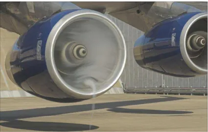
The ever increasing demand for quieter and more fuel efficient engines has lead to the need for higher by-pass ratio turbofans. As a consequence of this ongoing evolution in turbofan configurations, intake diameters are larger than ever before. For conventional wing mounted engines, in particular, this increase has major consequences. When the engine is operating in static or near static conditions close to the ground a strong vortex can be observed between the intake and the solid surface (Fig. 1.1). The ingested vor-tex is often invisible, however in humid conditions, due to the high velocities within the vortex core, the local flow temperature can decrease below the dew point, promoting condensation of the associated flowfield8.
Figure 1.1: Visualization of an ingested ground vortex on a Rolls-Royce RB211-524G cPeter Thomas 2005
This so-called ground (or inlet) vortex can be a major problem. With the advent of large passenger jets in the 1950s ground vortices were quickly identified as a prob-lem because of its ability to ingest large objects into the engine43,15. Low pressure in the vortex core can impart an impulsive force onto objects that are present on solid surfaces. Subsequently objects and also particles and dust (referred to as foreign ob-jects) are lifted off the surface, entrained into the inlet flowfield and carried into the engine by the induced velocity field of the intake. The ingested particles and debris
can damage fan blades, erode compressor blades and seals and degrade turbine cooling performance25.
However not only is the vortex responsible for foreign object ingestion (FOD), but it can also present a severe distortion of the associated intake flow-field33. This distorted flow-field can have a major impact on the aircraft performance, such as a reduction on the stall and surge margins and therefore compromising the safety of the aircraft. With fan diameters becoming increasingly larger, fan vibration has recently been iden-tified as an additional major consequence of ground vortex ingestion11,16. The non-uniform flow associated with the ground vortex entering the intake, introduces mo-mentum loss and large velocity gradients, which can significantly alter the local flow angle seen by the fan blade. As a consequence local flow separation can occur which leads to large resonant forces potentially resulting in high cycle fatigue.
1.1
Current Knowledge
It was previously identified that the key to the existence of ground vortices is the for-mation of a stagnation point on the ground ahead of the intake highlight plane43. In order for the aforementioned to exist, the capture streamtube must interact with the ground surface. This has been recognized to fundamentally depend on two key non-dimensional parameters. The first of which is the non-non-dimensional height of the intake,
H/Di, typically defined in the literature using the centreline height of the intake, H, and
the intake inner diameter, Di. The second dimensionless parameter is the velocity
ra-tio, Ui/U∞, which characterizes the contraction ratio of the sucked streamtube and is
a measure of the size of the streamtube upstream of the intake. This is derived from continuity considerations and is defined as being the intake velocity, Ui, divided by
the free-stream velocity, U∞. In order for the streamtube of the intake to interact with the ground plane the height-to-diameter ratio, H/Di, must be small and the contraction
ratio, Ui/U∞, must be large.
Current design rules for the avoidance of ground vortex formation relies on the vortex/ no-vortex map in which a number of previous researchers have correlated combinations of H/Di and Ui/U∞ for both when vortices are observed and when no vortex activity
is identified. This lead to the establishment of two distinct regions as a function of ground clearance and velocity ratio; a region of vortex formation and no vortex forma-tion (Fig. 1.2). At present this represents the most advanced designs rules for engine installations and operations. However, this graphic gives no indication of what happens to the quantitative vortex characteristics as the engine operates in different regions of the vortex formation zone (Fig. 1.2).
In terms of alleviating the phenomenon a number of methods, past and present, have been attempted with a number of patents being documented29,51. The majority of these measures attempt to remove the stagnation point on the ground plane which is
recog-H/D
iU
i/U
∞ 0.9 1 1.1 1.2 1.3 1.4 1.5 0 5 10 15 20 25 30 NO VORTEX VORTEXCurrent design trend
Figure 1.2: Velocity ratio against non-dimensional revealing a region of vortex formation nized as being a fundamental to the formation of ground vortices. Most mitigation measures use a jet of air, extracted from the compressor, directed on the region of vor-tex formation on ground, at an aim of removing the FOD issue. A prevention system, of this form, was even put into practice in the late 1950’s, and early 1960’s, on the DC-829,25. However after reviewing the unscheduled removal of engines due to FOD, the device was found to actually cause more problems by disturbing just as much debris as the vortex itself25.
Despite a number of flow control methods being developed, the general consensus is that ground vortex formation is unavoidable. With the current design trend of tur-bofans, intakes are operating further to the left in Fig. 1.2 in which the formation envelope is considerably larger. As a consequence ground vortex formation will occur over a wider range of operating conditions and will potentially be sustained for longer periods during the take-offphase. This significantly increases the number of vortex in-gestion events that will occur over the lifespan of the engine. With limited quantitative information available particularly at different height-to-diameter ratios, it is becoming vitally important to further understand the severity of the vortex in different regions of the vortex zone (Fig. 1.2).
1.2
Project Aims and Objectives
The present work primarily aims to provide quantitative information on the ground vortex over a wide range of operating conditions, which encapsulates the potential
changes in turbofan installations. In achieving this aim it is hoped that advanced design rules can be established for future engine designs. A number of key objectives have therefore been established to achieve this target:
1. Design and build a test rig for taking quantitative measurements of the ground vortex, at a representative intake Mach number, in the Cranfield University 8′×6′ wind tunnel.
2. Successfully apply the measurement technique of Stereoscopic Particle Image Velocimetry (SPIV) to the complex flowfield.
3. Conduct an extensive total pressure survey within the intake duct, for supporting analysis, for the majority of SPIV configurations.
4. Quantify the effect of the non-dimensional parameters of primary importance (i.e. the non-dimensional height (h/Dl), the intake yaw angle (ψ) and the velocity
ratio (Ui/U∞) in terms of vortex strength and fan face distortion.
5. Develop an empirical model that can predict the vortex characteristics for a given configuration.
6. Establish a more complex vortex formation map which can indicate not only when a vortex is expected to occur but also how detrimental it is expected to be for a given non-dimensional height and velocity ratio.
7. Provide the vortex characteristics of primary importance with regards to fan vi-bration (i.e. the vortex size, strength and intake distortion) and to understand how these vary with intake configuration.
8. Quantify and understand the effect of a moving aircraft on the formation and characteristics of the ground vortex using a rolling ground plane in the wind tunnel. This should reveal additional features on the formation mechanism as well as indicating the expected characteristics and lifetime of the vortex during the take-offphase.
C H A P T E R
2
Literature Review
A concise review of published work relating to ground vortex formation is presented in this chapter. The first part of the review discusses the criteria for vortex formation based on previous research. This is then followed by a discussion of the formation mechanisms that have been established to date, as well as the generation of ground vortices under reverse thrust operation. The review also includes CFD studies that have been published in the public domain. The chapter concludes by discussing the attempted methods of removing or reducing the impact of ground vortex formation.
2.1
Criteria for Vortex Formation
Within the first published works on ground vortex formation, characteristics, and be-haviour, it was quickly identified that a necessary requirement for vortex formation is the existence of a stagnation point on the ground plane43. This acts as a focal point for vorticity upstream to be concentrated and stretched into the intake. A prerequisite for this stagnation point to exist is that the sucked streamtube has sufficient interaction with the ground surface. The sucked (or capture) streamtube itself is defined as being a streamtube of air which divides the airstream into an internal flow and an external flow (Fig. 2.1). All flow inside the capture streamtube is ingested, whereas all air outside this boundary travels downstream. The characteristics of the sucked streamtube can be estimated from conservation of mass:
ρ∞A∞U∞ =ρiAiUi (2.1.1) A∞ Ai = ρi ρ∞ Ui U∞ (2.1.2)
For an incompressible flow the area ratio, A∞/Ai, of the sucked streamtube is equal to
the operating velocity ratio:
A∞ Ai
= Ui
U∞ =U
y
ρi
Intake outer surface
z
Edge of sucked streamtube
Di Ui U∞ Lq ρ∞ EXTERNAL FLOW INTERNAL FLOW
Figure 2.1: Illustration of sucked streamtube of an intake far from the ground
Within the literature on ground vortex formation, the velocity ratio, U∗, is used to
define the sucked streamtube size at far field relative to the intake dimension. When the approaching velocity, U∞, is low (i.e. U∗ is large) the engine mass flow demand increases and as a consequence the sucked streamtube size, A∞, increases to match this demand.
H U∞
z
Edge of sucked streamtube
Ingested vortex
Ui
y
Di
Ground plane
Figure 2.2: Schematic of the sucked streamtube interaction with the ground plane The primary parameters that dictate whether the capture streamtube interacts with the ground plane depends fundamentally on the height-to-diameter ratio, H/Di, of the
in-take (Fig. 2.2) and the velocity ratio, U∗ (which determines the size of the capture
streamtube at far field). High velocity ratios and low non-dimensional heights lead to an interaction of the streamtube with the ground and therefore vortex formation. The
dependency of these two parameters on the formation of ground vortices was graphi-cally illustrated by Liu et al31, in which pairs of H/Di and U∗ values were correlated
for cases with and without vortices. The vortex/no-vortex map reveals two regions; a vortex formation region and a no vortex zone (Fig. 2.3). Subsequently, in a related study, Shin et al50 constructed a vortex formation map based around Liu et al’s re-sults but also included data from full scale engine visualizations and other researchers. The established threshold has also been indicated in Fig. 2.3. In addition, Nakayama and Jones37 presented a criterion based on previous research (Eq. 2.1.4). This is also included in Fig. 2.3. All three datasets show excellent agreement, however they all appear to be based on roughly the same data.
Ui U∞ = 24· H Di ! −17 (2.1.4)
Nakayama and Jones37 presented quantitative total pressure measurements at two ve-locity ratios under headwind conditions with both data points being included in Fig. 2.3. Their results contradicted all the aforementioned thresholds with the data sug-gesting that a vortex can form at lower than previously reported velocity ratios (Fig. 2.3). At this point it should be noted that both the formation criterions established by Liu et al31 and Shin et al50 were based purely on crosswind configurations and were determined from visualizations only and as stated above the boundary presented by Nakayama and Jones appears to be based primarily on the same data.
H/Di Ui /U ∞ 0.9 1 1.1 1.2 1.3 1.4 1.5 0 5 10 15 20 25 30 Shin et al Brix N & K Glenny Motycka Liu et al Liu et al boundary Brix boundary (ψ= 90°) Brix boundary (ψ= 0°) Shin et al boundary N & K boundary NO VORTEX VORTEX
Figure 2.3: Correlation of velocity ratio and non-dimensional height combinations revealing
a region of vortex formation and no-vortex formation (filled symbols represents a data point in which no vortex is seen, and unfilled symbols are points in which vortices are observed)
More recently Brix et al6 presented a vortex formation map with a criterion being established for both headwind and crosswind configurations. Both have been approx-imately extracted and included in Fig. 2.3. Within Brix et al’s6 work quantitative
measurements were taken within the intake duct using a rotating hot-wire. However it is unknown whether this criterion was based on visualizations or quantitative results. Nonetheless there is a considerable difference between the established boundary un-der crosswind conditions (ψ = 90◦) and the previously mentioned vortex avoidance
thresholds. This discrepancy can be put down to the different methods used to detect a vortex, as well as potentially different operating conditions (such as boundary layer thickness). However, surprisingly the minimum velocity ratio required to generate a vortex under headwind conditions is higher in comparison to crosswind. No explana-tion was provided by the author for this observaexplana-tion. A number of possibilities could explain this finding such as different sucked streamtube characteristics between head-wind and crosshead-wind configurations, the crosshead-wind vortex being significantly stronger and therefore easier to detect, or that the unsteadiness is larger under headwind condi-tions, thereby rendering it’s presence difficult to determine.
A recent computational study by Jermy and Ho24examined the sensitivities of different upstream conditions on the formation boundary under headwind conditions. Within this research different upstream velocity gradients and approaching boundary layer thicknesses were examined. The authors found that ’no discernible vortex’ formed when the upstream shear reduced below a certain threshold24. However as will be dis-cussed below, previous experiments have shown that vortices can form under quiescent conditions, in which there is no upstream shear or vorticity source at all. In terms of the approaching boundary layer thickness, δ, results showed that as δ increased the vortex formation threshold was found to reduce24.
The above findings lead to an important point in terms of the observed sensitivities in the formation boundary. The velocity ratio defined by Jermy and Ho24 and within all previous literature uses the velocity ratio based on the free-stream velocity, U∞. However Eq. 2.1.3 derived above inherently assumes a uniform velocity profile within the sucked streamtube. If there is an approaching boundary layer present in the capture streamtube the velocity profile is therefore clearly not uniform, and will consequently have an effect on the sucked streamtube size. In order to ingest the same mass flow, the sucked streamtube area must increase. As a consequence, the velocity ratio (U∗) at
which the streamtube lifts offthe surface will be lower, as observed by Jermy and Ho24. Strictly, since the velocity ratio is a measure of the sucked streamtube contraction ratio the area weighted average velocity, ¯U∞, within the sucked streamtube should be used in the definition of the velocity ratio. Using this definition should give the same velocity ratio for any approaching boundary layer thickness. This is believed to be one of the reasons for the discrepancies in the observed formation boundaries∗. However since
the size of the sucked streamtube is generally not known, it is difficult to determine the ¯
U∞, and is why all published literature uses the free-stream velocity.
In addition to the necessary condition that the sucked streamtube interacts with the
∗The other main reason for the discrepancies in the formation boundary is the methods used to
detect the vortex. As stated above primarily flow visualization techniques have been used, however implementing such methods tend to only identify the strongest vortices. Hence weaker vortices that form just before the vortex is blown-away tend not to be identified
ground plane (thereby forming a stagnation point) all studies state that there must be a vorticity source for the vortex. Within the earliest reported studies a commonly quoted condition was the existence of ambient vorticity in the form of an approaching ground boundary layer9. However, as will be discussed in the following section, studies by de Siervi et al10 and Brix et al6 have revealed that vorticity can be introduced into the flowfield even with no approaching ambient vorticity source.
2.2
Mechanisms of Ground Vortex Formation
Research to date has identified two formation mechanisms. The first is applicable to an intake under quiescent (no-wind) and headwind conditions and the second relates to an intake in crosswind conditions. The two mechanisms are fundamentally different because of the contrasting dominant vorticity sources for the vortex. Consequently, comparatively different behavioural features and characteristics are observed with each respective mechanism which are described below.
2.2.1
Headwind Mechanism
This mechanism is applicable to an intake with its axis parallel to the flow direction. Many researchers have identified that it is the intensification of ambient vorticity that causes concentrated vortices to form. However it was not until the work of de Sievri et al10that proved this theory by conducting extensive water tunnel flow visualization studies using the hydrogen bubble technique. Different approaching vorticity sources and orientations were introduced upstream of the intake including a boundary layer, and clockwise and counter clockwise shear profiles (Fig. 2.4). It was shown that the direction, deformation and convection of the ambient vortex lines associated with the dominant vorticity source dictate the rotation and number of vortices seen at the fan face. This was also verified using potential flow theory in which the primary irrota-tional potential flow is superimposed linearly with a weak shear flow. Selected mate-rial lines were tracked as they approached the intake and the deformation of the vortex lines, where found to agree with the experimental observations. The flow topology for the different boundary layer profiles are discussed below.
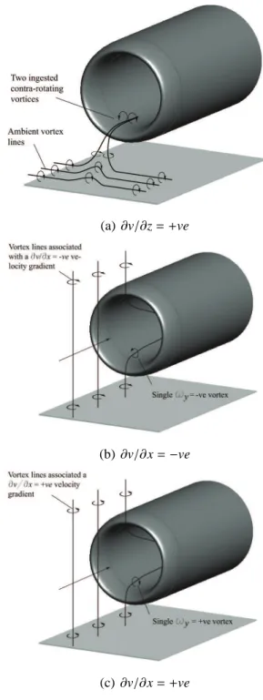
Vortex lines are defined as being a line in the fluid whose tangent is everywhere parallel to the local vorticity vector2. Hence for a boundary layer type profile (Fig. 2.4a) the vortex lines associated with this flowfield, far upstream of the intake, are parallel to the ground and perpendicular to the flow direction (Fig. 2.5a). As the vortex lines are convected by the mean flow and approach the intake they are stretched and deformed as illustrated in Fig. 2.5 due to the influence of the induced intake flowfield. As a result two counter-rotating vortices are ingested symmetrically placed about the intake axis (Fig. 2.5). The rotation of each respective vortex is directly determined by the rotation of the leg of the vortex line it is associated with (Fig. 2.5a).
y Intake outline z Ui Ground plane Upstream velocity profile ∂v/∂z = -ve (a) ∂v/∂z=−ve y Intake outline x Ui Upstream velocity profile PLAN VIEW ∂v/∂x = -ve (b)∂v/∂x=−ve y Intake outline x Ui Upstream velocity profile PLAN VIEW ∂v/∂x = +ve (c) ∂v/∂x= +ve
Figure 2.4: Velocity profiles used in de Siervi et al experiments (diagrams after de Siervi et
(a) ∂v/∂z= +ve
(b)∂v/∂x=−ve
(c)∂v/∂x= +ve
Figure 2.5: Deformation of the ambient vortex lines as they approach the intake for different upstream velocity gradients
In contrast, for the shear profiles the pattern is quite different. With a negative∂v/∂x
velocity gradient upstream (Fig. 2.4b) the vortex lines are straight and perpendicular to the ground surface (Fig. 2.5b). As they approach the intake, the high velocities associated with the intake flowfield stretches the vortex filaments resulting in only a single ground vortex being ingested (Fig. 2.5b). The rotation of the vortex is dictated by the corresponding rotation of the dominant vortex lines upstream of the intake. Hence with a negative∂v/∂x dominant velocity gradient upstream, the vortex rotates
in the intake duct such that it has negativeωy vorticity (Fig. 2.5b). The converse is
true for the positive∂v/∂x dominant velocity gradient upstream (Fig. 2.5c) where the
ingested vortex rotates with positiveωy. In addition to the experiments potential flow
calculations were performed to verify the experimental observations and to determine the behaviour of the upper legs of the ingested vortex lines. The results showed that the all the lower legs were concentrated at the stagnation point whereas the upper legs fanned out over the top of the intake, with no concentration being observed.
The experiments and theories put forward by De Siervi were instrumental in the under-standing on the fundamental mechanisms of vortex formation. However these studies were purely qualitative in nature and no quantitative information of the vortex was pro-vided. In order to determine the scale of the problem, distortion and vortex strength measurements need to be taken.
As a follow on to de Siervi et al’s10 research, Shin et al49 performed experiments to quantitatively verify the potential flow calculations. A negative∂v/∂x velocity gradient
was introduced upstream of the intake (Fig. 2.4b) and hot-wire measurements were taken inside the intake for a single configuration. The results confirmed the theory that the orientation and rotational sense of the ambient vertical vortex lines determines the number and rotation of the vortex within the intake. In addition, a first measure of the vortex strength was given for a H/D=1.13 and Ui/U∞ =22:
Γ
ω∞A∞ ≈ −2 (2.2.1)
However, it was not until the work of Brix5,6 that significant measurements of the ground vortex were taken. Quantitative data was taken inside the intake duct using two rotating hot-wires. The technique enabled quantitative measurements to be taken within the intake duct without averaging. The results were in agreement with the above observations, with some new findings also being reported. Perhaps the most significant of which was the formation of two contra-rotating vortices under quiescent conditions (U∗ = ∞), which had never been previously reported. Although no quantitative
mea-surements were presented under such conditions the vortices were observed to rotate in the opposite sense to that in headwind conditions. Brix et al6 also demonstrated quantitatively under headwind conditions that the vortices rotate in accordance with the quiescent mode if the velocity ratio exceeds a certain threshold. In the following section these flow modes are discussed in more detail.
2.2.1.1 Formation Modes
Under quiescent (no-wind) conditions the engine induces an external flowfield to the intake that emanates from all directions in the near vicinity. The induced velocities immediately adjacent to the ground interact with the surface generating vorticity. This ’induced’ vorticity is the source for the vortex and by definition this formation mech-anism requires no ambient vorticity. Brix notes that under no-wind conditions it is the flow behind and between the intake and the ground that dominates. As a conse-quence the vortex lines associated with this dominant flow are stretched and deformed as shown in Fig. 2.6. This situation is very similar to the headwind mode (Fig. 2.5a) except the source of vorticity is associated with flow approaching from the opposite direction and is a direct consequence of the intake induced flowfield rather than the approaching flow. As a consequence the vortices within the intake duct rotate in the opposite direction to that under headwind conditions, as shown in Fig. 2.7a. Since the formation mechanism is largely the same in comparison to headwind conditions, the vortices generated under quiescent conditions can be regarded as a flow mode of the headwind mechanism. This finding, by Brix et al, was purely based on flow vi-sualization studies and no quantitative measurements have been reported under such conditions to date.
Figure 2.6: Vortex formation under quiescent conditions
Related to the current work Murphy et al36 have quantitatively verified the findings of Brix. Using Stereoscopic Particle Image Velocimetry (SPIV) the flow under quiescent conditions was quantitatively studied and two contra-rotating vortices were found to form in accord with the flow topology presented in Fig. 2.6. However the flowfield was observed to be highly unsteady and often only a single dominant vortex was observed. For the first time quantitative measurements under quiescent conditions were presented which included fully averaged total pressure distortion measurements at the fan face. The vortices generated under quiescent conditions were observed to be weak but not insignificant.
In addition to the above findings, Brix et al6 quantitatively demonstrated that even under headwind conditions (i.e. U∗ , ∞), if the velocity ratio is large enough the
(a) No-wind mode (b) Transition phase (c) Headwind mode
Figure 2.7: Flow modes observed under headwind conditions (diagrams after Brix et al6)
vortices will rotate in agreement with the quiescent mode within the intake duct. This was shown for a configuration in which the intake height, H/Di, was equal to 1 and
the velocity ratio was U∗ = 33. In contrast, at a velocity ratio of 12 the vortices were
found to rotate in the expected fashion for the headwind mechanism (i.e. in accord with the flow topology presented in Fig. 2.5a and Fig. 2.7c). Brix noted that in between this rotation switch there existed a transitional phase in which the influence from the approaching (Fig. 2.5a) and induced vorticity sources (Fig. 2.6) are approximately equal and opposite (Fig. 2.7) leading to an instability in the vortex pair. The exact velocity ratio at which this occurred was not given in Brix et al6.
2.2.1.2 Additional Observations
Before the works of de Siervi and Brix an intriguing study was provided by Bissenger and Braun4in which contrasting observations are reported in comparison to the above findings. Similar to de Siervi et al10, hydrogen bubble visualization was implemented within a water tunnel but with a considerably smaller intake diameter, Di, of 16mm
constructed from a copper tube. A range of intake configurations were investigated including a single inlet close to the ground as well as two symmetrically placed inlets with no ground plane to examine the influence of the approaching boundary layer. For the single intake configuration, at low velocity ratios when no ground vortex was present two vortices were ingested into the intake and trailed downstream (Fig. 2.8a). This flow structure has never been reported by any other researchers. As the intake velocity and hence velocity ratio increased a vortex system appeared which comprised of a single ground vortex, a trailing vortex and a number of ground based streamwise vortices (Fig. 2.8b). Bissenger and Braun found that all vortices were non-stationary and often the ground vortex would appear on the other side of the intake with a re-versed sense of rotation (with the trailing vortex also reversing its position and rota-tional sense). Often the vortex system was observed to break down and then reform sporadically without any changes in the test conditions.
As stated above, the observations of Bissenger and Braun4 are slightly different to previously mentioned experiments. It should be noted that no upstream velocity profile
(a) Low velocity ratios
(b) High velocity ratios
Figure 2.8: Flow topology observed by Bissenger and Braun4under headwind conditions for (a) two trailing vortices (b) A complex vortex system involving a single ground and trailing vortex, plus vortices on the ground