Modelling inflation: different goals call for different solutions

(1)

UNIVERSIT `

A DEGLI STUDI DI ROMA “LA SAPIENZA”

Facolt`a di Scienze Statistiche

Dottorato in Scienze Economiche

XXIII CICLO

Modelling inflation:

different goals call for different solutions

Docente Laureanda

Chiar.mo Prof. Marco Lippi Claudia Paparo

Coordinatore

(2)

(3)

Abstract

Analysing prices behavior is not a unambiguous matter, it requires different methodologies depending on the aim of the study, on the period of time considered and on the available data. In what follows, we explore three different ways to model prices dynamics responding to alternative aims. We start from considering sector-level inflation indexes identifying the method still used in the Banca d’Italia to conduct the NIPE exercise; secondly, we consider individual prices in order to assess the degree of price stickiness in France, Germany and Italy using a factor model able to identify the effects of different kinds of shocks on prices at different level of aggregation; finally, we test the ability of the factor model in forecasting the overall inflation index of the same three Euro countries finding a significant forecasting power in the unobservable factors. Our results confirm that the data and the period of time considered can lead to quite different outcomes; moreover, different models can alternatively be the most precise in foreseeing inflation depending on the horizon of prediction or the country considered. In conclusion, the best way to analyse prices behavior is peculiar to the aim of the study: different methodologies, in fact, can be the most appropriate for different exercises.

(4)

Introduction

The controversial results obtained when trying to model price changes make forecasting inflation one of the most widely investigated issues in econometrics.

Analyses on inflation behaviour can be conducted in different ways depending on the aim of the study, on the frequency at which predictions have to be updated, on the country analysed and on the period of time considered. In what follows we are going to explore different ways to analyse prices behaviour: a sector-level indirect approach used at the Banca d’Italia to frequently update national inflation predictions, a more disaggregate approach starting from individual series (not only prices) summarised in a factor model in order to assess the persistence degree of inflation in the three largest Euro countries, a direct approach comparing alternative models accuracy in forecasting the same national inflation indexes.

The results clearly confirm that the best way to model inflation dynamics is peculiar to the country and to the period of data considered; moreover, different econometric specifications can give more accurate results in catching the influence of macroeconomic shocks hitting the economic system at different horizons.

The interest on price dynamics has increased since 1999, when the euro has been adopted as single currency and the European Central Bank (ECB) has been charged with maintaining the euro’s purchasing power and thus price stability in the euro area. This objective is accurately specified in the following statement that defines the so-called ‘inflation target’: ‘an annual Harmonized Index of Consumer Prices (HICP) inflation rate of below, but close to, 2% over the medium term’ (ECB [1]). In order to successfully achieve this goal, the European Central Bank calls for a continuous monitoring of inflation developments in the euro area. To this aim the Eurosystem runs every quarter an exercise in which each National Central Bank (NCB) produces a national inflation forecast for a relatively short forecast horizon, varying from 12 to 15 months. The forecast target is the year-on-year growth rate of the Harmonized Index of Consumer Prices. This exercise, named Narrow Inflation Projection Exercise (NIPE), runs parallel to a more articulated one (the (Broad) Macro Projection Exercise) which goes well beyond the NIPE horizon (up to three years ahead) and covers a large number of macro variables.

(7)

In fact, although the inflation target refers to the medium term and is related to structural economic conditions, it is useful to consider a short term intermediate objective because it gives a faster indication of the economic situation thus permitting a prompt intervention in case of relevant deviations from the final target.

There are alternative methods to obtain a valid forecast for the overall HICP index:

• modelling the aggregate index in order to obtain a direct projection, getting a rapid esti-mate of the expected price growth;

• conducting a forecasting exercise on each sub-index, computing the overall inflation as a weighted sum of the sectors’ prices growth rates;

• considering all the available information about the economy summarised in a small number of common factors driving macro aggregates as inflation.

The indirect approach has the advantage of taking into account the different variables that influence the price change in each main sector: typically, sectors as clothing and unprocessed food are strongly influenced by seasonality, because of periodic events as sales and climatic changes respectively. Moreover, this strategy has an econometric advantage, as Clements and Hendry [29] show: aggregating forecasts can lead to more accurate results, because the erratic component present in each single price series tends to cancel out. It is still not clear whether the direct or the indirect method would be the most accurate, as different papers have been published supporting one strategy or the other (see the Section 1.1). Alternatively, a factor model avoids

any a-priori choice about the economic variables to include in the models. Integrated markets

and common monetary policies have made economies much more interdependent, so that shocks influence is mutually pervasive across countries; in order to consider all the available information, a factor model identifies a small set of macroeconomic shocks driving economic indicators out of a large number of observable series regarding every aspect of the economic system.

In Chapter 1 we follow an indirect approach to conduct the NIPE exercise, identifying the most accurate forecasting models for the main HICP sub-indexes: Services, Goods, Energy, Processed and Unprocessed Food. For each of these sectors, different linear models have been compared, alternatively testing the forecasting power of various economic variables that could significantly influence price changes. In order to choose the best model in predicting inflation, we consider the specification with the minimum Root Mean Squared Forecast Error (RMSFE) at different horizons. Additionally, the chosen model has been compared with a na¨ıf model: for particularly erratic HICP sectors as the Energy component this specification is still hard to overcome in terms of forecasting accuracy. In Chapter 1 we report the final model selected for each sub-index and the relative forecast errors from 1 to 15 steps ahead. In order to obtain the

(8)

overall expected inflation, the contribution of each component to the predicted price growth will be added up according to the weights of each sector in the HICP composition.

The good performance of the indirect approach in terms of predictions accuracy can be further exploited analysing individual-level economic series regarding every aspect of the economy, not only prices. Important information about unexpected shocks influencing macro aggregates as inflation can be provided by labour, financial and house market indicators; moreover, analysing prices at different levels of aggregation can provide different results in terms of inflation dynam-ics.

As pointed out in previous works such as Boivin, Giannoni and Mihov[21] and Altissimo and Zaffaroni[5]1, price responses are quite heterogeneous across different sectors: energy and unpro-cessed food prices are quite volatile, while goods and services prices change quite infrequently; moreover, price dynamics result to be quite different depending on the level of aggregation of the series. In Chapter 2 we analyse the price series behaviour in the three largest EU countries considering both aggregate and sectoral inflation: the former results less volatile, supporting the sticky price traditional evidence in the short run, while disaggregated series, considering both consumer and producer prices, result more flexible in responding to economic shocks.

The reason of the different price behaviour is in the different kinds of shocks hitting the economy. Recent empirical investigations have shown in fact that disaggregated price series in US appear to be sticky in response to macroeconomic shocks, but they come back to the equilibrium level quite rapidly after a sector-specific shock. Given that these sector-specific shocks are responsible for most of monthly price fluctuations, the series result quite volatile, in contrast to the theoretic hypothesis of most of economic models.

We follow Boivin, Giannoni and Mihov[21] using a factor-augmented vector autoregression model consisting in estimating a small number of factors summarising the economic dynamics out of a large data set of monthly and quarterly series. This model allows us to disentangle the impact of a shock on the common and idiosyncratic component of inflation. Moreover, we investigate the impact of monetary policy on disaggregated inflation identifying a monetary shock by using information from the entire data set.

We conduct the analysis comparing inflation dynamics in the three largest Euro countries, namely France, Germany and Italy, that represent more that 65% of Euro Area’s GDP. Moreover, they joined the Euro Monetary Union from the beginning, so statistics are available and complete in the main European databases. Unfortunately, some kind of data is not available in any European database in an homogeneous form and has to be gathered from each national institute of statistics. Each institute considers different categories of products and with a different level of

(9)

disaggregation, hence in order to obtain a uniform database, series have to be made comparable by product type. Time availability is another shortcoming of European data: while US price series are available for more than thirty years’ time, unfortunately European series start only from early 90s.

The results are quite similar for the three countries, both for CPI and for PPI series, apart from French PPI indices that deserve particular attention. Aggregate inflation shows low persistence and volatility mostly due to the macroeconomic component. The idiosyncratic component, instead, is responsible for most of the disaggregated prices fluctuations. On one hand, our findings about inflation volatility are similar to those from previous works; on the other, the degree of price persistence, considering both aggregate and disaggregate series, results much lower. In contrast to Boivin, Giannoni and Mihov[21], we don’t find that macroeconomic shocks have a significant impact in the long run: individual prices in fact result to be quite flexible in absorbing a monetary shock. The explanation of this apparent contradiction is in the positive correlation between inflation and persistence: estimating the same model on a period of low inflation (as the one we have experienced since the creation on the Eurosystem) or on a longer span of data including periods of high inflation (as Boivin, Giannoni and Mihov[21] do using US data) can produce very different results in the shock persistence degree.

Given that the FAVAR model provides useful information about prices dynamics, a further step is to test its forecasting ability in correctly estimating future changes in price levels. In Chapter 3 we illustrate the forecasting accuracy of the factor model compared to several alter-natives when applied to the same data used in Chapter 2. Though different models result to best predict inflation in the three countries, a factor model that summarises all the available information in a few artificial variables imposing very few restrictions on agents’ behaviour re-sults to be significantly useful in correctly foreseeing the future price trend. Moreover, we test the forecasting performance of different models from 2008 to 2009, that is when the economic crisis started hitting the EU countries causing quite serious drawbacks. The predictive accuracy of the factor model in a period characterised by high uncertainty enforces the belief that it is a very useful tool for modelling price behaviour.

The results confirm that combining forecasts from different models can significantly improve the forecasting performance, given the relative accuracy each specification has over different sub-periods. Moreover, a forecast combination substantially reduces the uncertainty associated with monetary policy decisions, in line with the literature that encourages for the most complete use of information available in the economy. Therefore, a factor model including artificial variables that summarise all the shocks affecting the economy can provide quite accurate predictions.

(10)

by many Central Banks, like the Banca d’Italia (as described in Chapter 1) and the Bank of England. Kapetanios et al.[41] illustrate the different models composing the so-called ‘Suite of Statistical Forecasting Models’, ranging from pure statistical to data-free theoretical models. The different forecasts are then summarised using a system of weights based on the AIC infor-mation criterion, because different models can be differently affected by the shocks hitting the economy.

The exercise confirms the peculiar nature of forecasting inflation: different models result to be the most accurate at different horizons or for alternative measures of inflation. Unobserva-ble factors taking into account different shocks hitting the economy have predictive power espe-cially at medium and long horizons, while univariate models are more accurate at short horizons. Moreover, different models can result more useful depending on the national inflation index iden-tified as the variable to forecast: we find that Italian HICP is precisely predicted with a factor model, while for the German corresponding series can be more useful a moving average of the first largest factor only.

The forecasting exercises described in Chapters 1 and 3 are not completely alike. Even if they are both driven by the comparison between alternative models in terms of Root Mean Square Forecast Errors, in the former only sector-level prices are considered and the best model for each sub-index is chosen on both statistical and economic basis. The aggregation level and the model selection procedure are chosen in order to respond to the ECB request and to make more explicit the variables driving each component. Abrupt exogenous shocks can influence some sectors only; therefore, the indirect approach provides an easier understanding of the effects of unpredictable disturbances occurring in the economy. On the other hand, setting up and frequently updating a wide data set composed by individual series regarding every aspect of the economy (as the one used in Chapter 3) can result quite time-consuming; moreover, changes in the loadings of unobservable factors could be quite difficult to identify in changes of underlying variables in order to provide an economic explanation of wrong predictions. Considering hundreds of disaggregate series can be useful if otherwise the aim of the exercise is computing proxies of common macroeconomic shocks hitting economies having a common monetary policy as the Euro area. The same ECB decision of intervention can have quite variable effects on the EU countries depending on the transmission mechanism of monetary policy differently affecting national economies and in particular price levels. Besides, considering all the available data allows to avoid a priori choices of the variables to include in the model implying the exclusion of a relevant set of information about the country.

In conclusion, analyses on inflation dynamics can be conducted in different ways depending on the goal of the study: different needs require appropriate solutions that can differ in methodology,

(11)

data and obviously results. In what follows we explore three different ways to analyse price dynamics: starting from the indirect approach implemented at the Banca d’Italia focused on the HICP main sub-indexes, we deepen the analysis considering individual series in order to investigate the stickiness degree of prices at different levels of aggregation and we conclude assessing the predictive power of unobservable macroeconomic shocks directly forecasting three EU countries HICP index.

(12)

Chapter 1

Inflation in Italy: models for the

NIPE

1.1 The NIPE

As anticipated in the Introduction, the Narrow Inflation Projection Exercise required by the ECB consists in producing inflation forecasts for a relatively short predictive horizon.

The approach behind the NIPE is bottom-up: each country is required to produce a forecast for five sub-indexes: non-energy industrial goods (henceforth NEI-goods), services, processed food, unprocessed food and energy goods, which are subsequently aggregated into a headline inflation projection. A distinctive feature of the exercise is its conditional nature. Inflation forecasts are linked to the development of some important international variables whose path over the forecast horizon is assumed as given: the oil price, the nominal effective exchange rate, the US dollar/euro exchange rate and the prices of internationally traded commodities.

As we previously pointed out, whether the bottom-up approach leads to more accurate fore-casts than a direct projection is still a controversial matter. According to Benalal et al. [12], modeling each component can be convenient at short horizons as it allows to follow the peculiar patterns that characterise each sub-index, but its effectiveness is not assured. Using monthly series from 1990 to 2002 for both the HICP components and for the overall index, they estimate a forecast model minimizing the RMSFE of recursive dynamic out-of-sample forecasts. This statistic has been calculated for different horizons, namely 1, 3, 6, 12 and 18 months ahead. Different models can result as the most accurate depending on the time horizon considered, so they average the 5 RMSFE in order to obtain a unique selection criteria. They compare both univariate and multivariate (VAR and BVAR) linear models, finding that the indirect approach is slightly more precise for 1 and 3 months ahead forecasts; the longer the horizon, the better the

(13)

direct approach results. Considering instead the overall index excluding energy and unprocessed food, the indirect approach outperforms the direct forecasting at all the horizons. In conclusion, considering each component separately seems to be meaningful if applied to short horizons or if used to predict the core inflation index.

Moreover, theoretical reasons in favour of aggregating the forecasts of the subindexes argue that in the aggregation process the forecast errors can cancel between components (Clements and Hendry [29]). Pooling of forecasts may pay dividends by averaging offsetting biases: different models, in fact, are differently affected by unanticipated shifts. Even if it is not easy to prove that a forecasting combination can improve over the best model selected for the overall index, the authors show that averaging does reduce variance, as long as different sources of information are used. It can be interpreted as an intercept change over a baseline model: each component gives a contribution in terms of forecast accuracy to improve the model that best fits the overall price series in case of structural breaks and deterministic mis-specifications.

Empirical applications, however, suggest that this is not always the case. Hubrich [39] uses a wide range of models and selection procedures and finds that aggregating inflation forecasts by components does not always improve the model’s forecast accuracy twelve months ahead. The author argues that direct forecasting is a superior method to obtain precise predictions: disaggregated models can be mis-specified, so that they do not improve the forecasting accuracy of the aggregate, especially if some exogenous shocks occur. The author tests different model selection procedures over different forecast horizons using different inflation measures, analysing both the overall HICP index and its core component. Evaluating each model forecasting per-formance using Monte Carlo simulations for one to twelve steps ahead, Hubrich [39] obtains mixed results: for a short time horizon, aggregating sub-component forecasts outperforms the direct prediction, while for six to twelve months ahead modeling the aggregate inflation index produces more accurate projections. It seems that, as the forecast horizon gets longer, the pre-diction errors of the sub-components do not cancel out: the different models tend to react to exogenous shocks in the same way so that the forecast bias is not reduced aggregating the sub-indexes. A different result is obtained excluding the most volatile components of HICP, namely energy and unprocessed food, and considering as overall index the so-called ‘core’ inflation. In this case the indirect approach performs better even at long forecast horizons: aggregating sub components forecasts is not recommended when some components are strongly volatile and so hardly predictable.

Hubrich and Hendry [40] also find mixed results when using disaggregated information to forecast directly headline inflation. They suggest to include information from disaggregated variables in the aggregate model instead of first forecasting each sub-index separately and then

(14)

aggregating those predictions. Model selection plays an important role in determining the effec-tiveness of disaggregated variables; moreover, the more the aggregate and the components are variable in the estimation sample, the more the combined estimation improves the forecast accu-racy. The authors forecast euro area and US inflation using data from 1992 to 2001 comparing the predictive power of different models: using only the aggregate, indirectly aggregating sub-components forecasts and finally including the sub-components into the model for the aggregate as explaining variables. Simulated out-of-sample forecasts show that including disaggregated vari-ables in the aggregate model does improve predictability especially at long forecasting horizons. Moreover, practitioners might find forecasting directly aggregate inflation more convenient for other reasons. First, model specification search can quickly become daunting when one considers a high level of disaggregation. Second, since forecast models need to be continuously fine tuned having a single tool is an obvious advantage. Third, breaks and seasonality are less of a problem in aggregate than in disaggregate data.

In practice, although monetary policy in the euro area ultimately targets headline year-on-year inflation over the medium term, the bottom-up approach allows a clearer reading of the underlying inflation signal. Temporary abrupt exogenous shocks can lead to strong base effects with consequent hump-shaped behavior of inflation over the forecast horizon which can be easily reconducted to some underlying components. Recent developments in food and energy prices provide a good example of the added value of considering separately some of the items in the consumption basket. In this respect the disaggregate approach makes the story behind the aggregate figures more explicit. Moreover the transmission mechanism of monetary policy or exogenous shocks to sub-components may differ substantially, as tradable goods are likely, for example, to be influenced by the exchange rate more than services (Aron and Muellbauer [8]). Moreover, the indirect approach allows to use a wider information set specific for each subcomponent, given that the level of competition, the taxation burden and the technological improvements can be different in each sector. While the real exchange rate, labour costs and producer prices are significant for both durable and non durable goods, the union density affects only the second; on the other hand, the service sector equation is the only one where the lagged overall HICP index results significant, evidence that this sub-component is particularly affected by the past aggregate inflation level.

In conclusion, as different HICP sub-indexes have different inflation histories, the indirect approach can substantially improve the forecasting accuracy of the aggregate series. Significant gains can derive from sectoral information, as the effects of exogenous shocks can be different on each component and the forecasting errors can cancel out in the aggregation process.

(15)

pro-jections and is structured as follows. In Section 1.2 we have a preliminary look at inflation developments in the past twenty years in Italy and justify our modeling strategy which consists of focusing on the period following the disinflation of the mid-Nineties. In Section 1.3 we clarify the further refinement on the sub-indexes we use with the intent of separating market-based prices from administered ones. In Section 1.4 we describe the model selection criteria. In Sec-tion 1.5 we evaluate the models forecasting performance. In SecSec-tion 1.6 we look at the implied inflation elasticities to a shock to three exogenous variables, namely the nominal effective ex-change rate, the oil price and the price of internationally traded food commodities. Section 1.7 concludes.

1.2 Data description and some conceptual issues

The full breakdown of HICP official data is available since 1995. The main sub-indexes, however, have been back-linked for most countries on the basis of national CPIs and are available for Italy since 1987. The year-on-year percentage changes of the overall index and of the five sub-components used in the NIPE are shown in Figure B.1. It is clear that over the past twenty years the inflation process in Italy underwent a strong structural change dropping from an average of around 5% in the first decade to about half this value in the following one. A formal test (Andrews [6]) detects a break in the unconditional mean of the year-on-year inflation rate in June 1996. Visual inspection of the sub-components and a formal analysis confirm that the break is common to NEI-goods, services and processed food.1 Also notice that NEI-goods inflation presents two low spikes in 2001. These are due to a methodological change introduced by Eurostat which started recording prices inclusive of seasonal discounts. The effect of the introduction of sales price recording on the volatility of inflation rates is quantified in Table 1.1 in which we report the standard deviation of month-on-month rates of growth of NEI-goods, Clothing and Footwear and NEI-goods net of Clothing and Footwear indexes before and after 2001. Clothing and Footwear and NEI-goods inflation rates are twenty and ten times more volatile in the second sub-sample. If one excludes Clothing and Footwear, however, NEI-goods inflation results half as volatile after 2001, consistently with a reduction in volatility of price dynamics observed in the euro area countries since the inception of the monetary union. Figure B.3 shows that the rate of inflation of NEI-goods net of Clothing and Footwear displays indeed a much more regular behavior over the whole sample. We model Clothing and Footwear separately from other NEI-goods in our forecasting system.

1

The Andrews sup-wald break test detects a change in the constant in November 1996 for NEI-goods, in August 1996 for services and September 1996 for processed food.

(16)

1995-2000 2001-2008 NEI-goods 0.19 1.63 Clothing and Footwear 0.22 4.30 NEI-goods net of Clothing and Footwear 0.26 0.13

Table 1.1: The effect of sales prices recording on inflation volatility

Three main factors contributed to the observed change in aggregate price dynamics in Italy (Gaiotti [37]). First, wage indexation was abolished in 1992 and wage growth in collective bargaining was linked to the Government’s inflation target. Second, the attitude of monetary policy towards inflation turned more aggressive in 1995, with the announcement by the Governor of the Banca d’Italia in his annual statement between 1995 and 1997 of a level above which inflation would be intolerable. Third, financial market innovations strengthened the impact of monetary policy credibility on both long-term interest rates and the exchange rate. In summary, in the mid-Nineties a shift in the monetary policy regime towards inflation stabilisation, favoured by decisive changes in the structure of financial and labour markets, effectively anchored actual inflation to expectations. The occurrence of a structural break in the three main sub-items for which labour costs represent a large share of input costs confirms that the activation of an

expectation channel is behind the moderation of inflation since the second half of the Nineties.

Subsequently, the adoption by the ECB of an explicit objective of price stability reinforced the role of inflation expectations in price setting and contributed to keep price growth in Italy at historically low levels.

How to treat such a structural change when setting up a forecasting model is an open issue. Mixing observations across different policy regimes requires allowing for breaks in the parame-ters, which would complicate the models. Using samples across policy regime shifts also risks to overstate transmission lags and, consequently, inflation persistence. In the case of the euro area, for example, using a long sample and not allowing for breaks O’Reilly and Whelan [48] find that inflation is close to a random walk. However, using the same estimation strategy Benati [13] finds that inflation persistence since the start of the European Monetary Union has been close to zero. Our modeling choice was to model inflation under the current low persistence regime and therefore disregard data prior to 1997.

A further complication is given by the fact that the NIPE models need to be flexible enough to give a good forecasting performance on the very short-run (one to three months ahead), and also to be informative on the medium-run (twelve/fifteen months ahead). We illustrate this point with an example. Consider a model specified in year-on-year terms (like, for example, the

(17)

ones in Aron and Muellbauer [8]) in which year-on-year inflation twelve steps ahead is a function of current exogenous variables. The estimation equation of such a model is:

∆12log(Pt) =α0Xt−12+t (1.1)

where the X vector can include variables like unit labour costs, import costs, capacity utilisation and the exchange rate and ∆12 = (1−L12). The one month ahead forecast of this model is

given by:

∆12log(Pt+1) = ˆα0Xt−11 (1.2)

Equation (1.2) shows that in forecasting one step ahead we are disregarding all the information accumulated in the past eleven months.2 The most important information we are missing is current year-on-year inflation ∆12log(Pt) and the month-on-month inflation rate eleven months

before: ∆1log(Pt−11).

Using the following definition:

(1−L12)log(Pt+1) = (1−L12)log(Pt) + (1−L)(1−L12)log(Pt+1) (1.3)

= (1−L12)log(Pt) + (1−L)log(Pt+1) + (1−L)log(Pt−11)

it can be seen that, conditional on the current information set (which includes current year-on-year inflation ∆12log(Pt) and past month-on-month inflation ∆1log(Pt−11)) the accuracy of the

one step ahead prediction depends on the term (1−L)log(Pt+1) which is the month-on-month

inflation rate one month ahead. Since the (1−L) filter cuts off all the long-run information while retaining seasonal and very high frequencies, a model such as the one in (1.1) which is specifically designed to capture medium-term inflation and is motivated by economic theory is going to be outperformed by simple alternatives geared to high frequency fluctuations. Even a constant plus seasonal dummies is going to be a very hard competitor.

When modeling inflation for the NIPE one therefore lacks a clear loss function (whether to favour short-term or medium-term performance) and needs models that are a hybrid between purely statistical and economics-motivated ones. A viable alternative is to use different models for short and long horizons. Models specified in month-on-month terms could provide the initial condition to which forecasts derived from medium-term models could be linked. As we explain below we explore this possibility in modeling services inflation.

2

Current information could enter the equation via the parameterαwhich could be re-estimated every time. If parameters are stable, however the change inαinduced by new information is likely to be negligible.

(18)

1.3 The sub-indexes used at the Banca d’Italia

When trying to relate price developments to economic determinants a further problem is posed by the existence of prices which are not set on the basis of market conditions but are determined by Public Authorities. This is the case of some public services (like transportation) or of regulated monopolies. For these items (which fall in the category of administered prices) inflation follows Government decisions which are hard to predict.

Some other indexes are more suited to be forecast by purely seasonal models or simply by expert judgement. This is the case of Clothing and Footwear, whose volatility since 2001 is strongly affected by the timing of seasonal sales, or of telephone equipment prices, which are corrected for technological improvements and have therefore been constantly falling in the past ten years.

Considering these issues we further disaggregate the main HICP sub-indexes as shown in Table 1.2. There are two groups of sub-indexes that are explicitly modelled. In the first group there are items for which a forecasting model is developed and tested in a pseudo out-of-sample simulation exercise. In the second group there are items for which we develop a model that provides a reasonable fit but we do not explore forecasting accuracy, either because of recent changes in the tariffs schemes (as is the case of energy tariffs and air transportation), or of recent breaks (as for clothing and footwear). These indexes, however, either have a substantial weight in the basket (energy and clothing and footwear) or have a very volatile profile so that a basic model helps in tracing back some large occasional forecast errors (as is the case for air transport). The items that are excluded altogether (which represent around 7% of the overall index) are forecast either on the basis of information from the relevant price setting Authorities or on the basis of simple seasonal models.

1.4 Model selection criteria

As explained above, NIPE forecasts are conditional on a set of exogenous variables (interest rates, nominal bilateral and effective exchange rates, oil and other commodities prices) whose future path is determined at the beginning of each NIPE. Since the projections produced within the NIPE are conditional on these assumptions, in the out of sample forecast exercise below we use their actual value over the forecast horizon (for example, when projecting energy inflation we assume to know future oil price). Other exogenous variables used in the analysis either enter the equations with sufficient lags so that they do not need to be forecast or are forecast with an autoregressive model. Quarterly variables, when used, are linearly interpolated at the monthly frequency. An important issue is the timing of release of producer prices, which have a strong

(19)

FIRST GROUP

Sub-indexes modelled Excluded items Weight in the HICP

Telephone and fax equipments,

1 NEI-goods water and medical products, 18

clothing and footwear Transport

2 Services Refuse and sewerage collection 34

postal, telephone and education

3 Energy goods Energy tariffs 4

4 Processed food prices Tobacco prices 10

5 Unprocessed food prices 8.4

74,4 SECOND GROUP

6 Air transport 0.9

7 Energy tariffs 3.7

8 Clothing and footwear 12

Table 1.2: HICP disaggregation scheme used in the Italian NIPE system

predictive content for consumer prices but are released with one month delay. Whenever we specify a model that uses producer prices the latter are lagged by one month. We impose a similar constraint on quarterly variables which are intended aslagged by three months, given the delay with which they are published.

For each subcomponent we search across linear models based on observed variables. These two requirements rule out unobserved components models, time varying coefficients models (including Markov switching models). This allows us to attribute forecast revisions between two successive NIPE either to a change in the assumptions or to forecast errors, rather than to changes in unobserved components which would be hard to explain and would make the communication of inflation forecasts problematic. We therefore work with vector autoregressions (including long-term cointegrating restrictions when not rejected by the data), linear equations or systems of linear equations.

The variables chosen for each model are determined by economic criteria. All the models reflect an assumption of mark-up pricing and therefore relate consumer prices to their relevant costs or to cyclical variables which capture mark-up adjustments over the cycle. The specifi-cation search for energy and food inflation models is much less costly as energy and food price developments can be easily linked to oil and food commodity prices. Forecasting models for core

(20)

components (NEI-goods and Services) could instead contain domestic supply and demand side variables, as well as international prices: they therefore require a more careful model selection process, which we borrow from Aron and Muellbauer ([8]).

The analysis is conducted on data from 1997 to 2008: observations up to December 2004 are used for the model estimation, while the following sub-sample is used for recursive out of sample forecasts. Recursive forecasts are computed for a maximum of fifteen steps ahead and prediction errors are computed for both month-on-month and year-on-year inflation rates. The performance of our models on year-on-year inflation is checked against that of a random walk, which is known to be a tough competitor at low frequencies (Atkeson and Ohanian [9]). The performance on month-on-month inflation for one and two steps ahead is compared to that of a constant plus seasonal dummies. The reason for considering different benchmarks at different horizons relates to the issues highlighted in Section 1.2. On one hand we want our models to have more information than that contained in the seasonal pattern at very short horizons. On the other hand we want them to be able to track medium-term inflation developments.

In order to select the best specification for each model we use the three classical Schwarz (SC), Hannan-Quinn (HQ) and Akaike (AIC) information criteria and the root mean squared forecast error (RMSFE) both in sample and out of sample. In addition, following Den Reijer et al. [32], we also consider ‘mixed’ criteria, that is we compute the above penalties on a weighted average of in and out of sample errors (with weights equal to 0.6 for the in-sample and 0.4 for the out of sample). When these information criteria give conflicting results the best performing model in terms of ‘mixed’ AIC is chosen.

1.5 Modelling core items: NEI-goods and Services

1.5.1 Services

The best model at medium-term horizon is a single equation in year-on-year inflation rates. The main determinants of services inflation are found to be unprocessed food prices (relevant for the restaurants and bars component), the oil price (which impacts both through electricity costs and through fuel prices for transportation services), unit labour costs and real value added growth rate. Transmission lags of over a year from costs and cyclical variables to consumer prices are consistent with the evidence provided by Veronese et al. [54] which report a frequency of consumer price changes of about 14/15 months for services in Italy. In the short-run, on the other hand, the predictive accuracy of a VECM in services prices and unit labour costs is superior to that of a purely seasonal model. We therefore run the out of sample exercise combining forecasts from these models. To ensure a smooth link between the two we perform a

(21)

two months linear interpolation between the VECM and the equation forecasts (see Table 1.3). The results of the out of sample forecast exercise are shown in the first column of Tables A.1 and A.2. For year-on-year inflation rates our model outperforms the benchmark from the third step ahead onwards; moreover its predictive accuracy does not deteriorate for longer horizons. On monthly inflation rates our model also improves, albeit slightly, upon the naive seasonal model one and two steps ahead.

Horizon Model Endogenous Lags Endogenous Exogenous

∆log(puf_t₋₁₄) 1-2 VECM ∆log(pser₎_, _∆_log₍_ulc₎ _1,12 _∆_log₍_vaser

t−16)

∆log(poil_t₋₂₃)

3-4 Linear Interpolation

∆12log(psert−12)

∆12log(puft−12)

5-12 Single equation ∆12log(pser) ∆12log(poilt−18)

∆12log(vasert−13)

∆12log(ulct−16)

Table 1.3: Models for services inflation

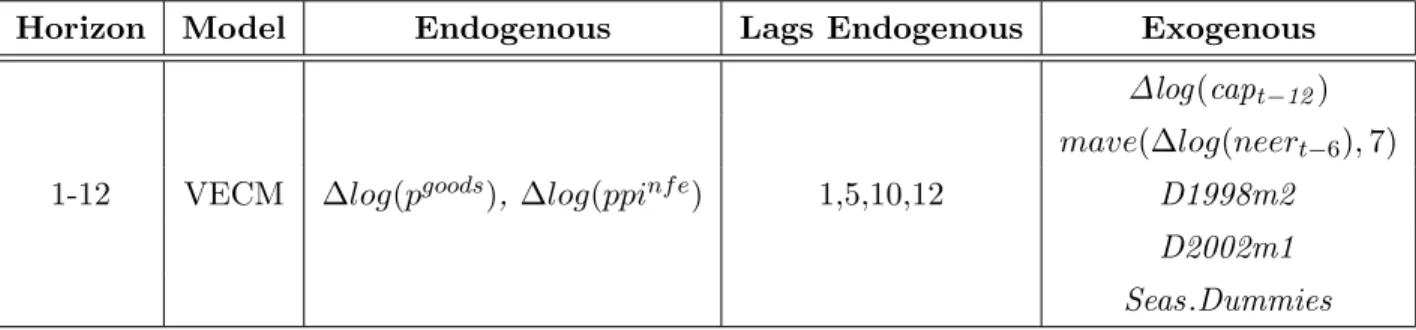
1.5.2 NEI-Goods and Clothing and Footwear

This component is particularly hard to model, given the increasing effect of foreign competition from emerging markets on domestic mark-ups (see Bugamelli et al. [23]). Since it was not possi-ble to establish a significant cointegration relationship between consumer goods prices and unit labour costs we resorted to a VEC model in goods and producer prices (net of food and energy) with capacity utilisation rate and a smooth transformation of the nominal effective exchange rate as exogenous variables (see Table 1.4). We also include two intervention dummies for February 1998 and January 2002. The model is in monthly rates and includes seasonal dummies. The second column of Tables A.2 shows that in terms of month-on-month rates the model and the naive benchmark deliver the same performance. The very low RMSFE (0.11) reflects the low volatility of the series. Despite being tailored to capture high frequency movements the VECM manages to outperform the naive benchmark also on year-on-year growth rates from the first step onwards (see the second column of Table A.1). Given their strong seasonal pattern clothing and footwear are modelled using TRAMO/SEATS. The resulting forecasts are more accurate

(22)

than the naive benchmarks both at monthly and yearly frequencies at almost all horizons (see the third column of Tables A.1 and A.2).

Horizon Model Endogenous Lags Endogenous Exogenous

∆log(capt−12)

mave(∆log(neert−6),7)

1-12 VECM ∆log(pgoods),∆log(ppinf e) 1,5,10,12 D1998m2

D2002m1

Seas.Dummies

Table 1.4: Model for non-energy industrial goods inflation

1.5.3 Food

Food prices have been particularly relevant for inflation dynamics in the euro area since the second half of 2007, when they accelerated in the wake of a strong growth of commodity (espe-cially wheat) and milk prices. Since detailed food commodity prices are part of the international assumptions used in the NIPE we use them to construct a food commodity index (FCI) that reflects as closely as possible their weight in the Italian consumer basket. In particular the index is a weighted average of international prices of cocoa, coffee, wheat, sugar, soybeans and milk. The matching of commodities with HICP sub-components and their respective weights is summarised in Table 1.5.

HICP sub-component Weight in the HICP basket Corresponding commodity

Bread and cereals 30.83 Wheat

Milk, cheese and eggs 23.63 Milk

Oils and fats 8.48 Soya beans

Sugar et al. 11.46 Sugar

Coffee, tea and cocoa 2.54 Coffee, cocoa

Table 1.5: Weights used to compute the Food Commodity Index

The FCI is used to model both processed and unprocessed consumer food prices, together with food producer prices. The best model specification, however, is different for the two sub-components: unprocessed food inflation is best forecast with a system of two equations. A

(23)

long moving average of the FCI monthly growth is used to predict food producer prices, which, in turn, enter the HICP equation (see Table 1.6). Processed food prices, on the other hand, are found to be cointegrated with producer prices with a unitary long-run elasticity. For this sub-component we therefore specify a VEC model in consumer and producer prices that uses a moving average of the FCI as exogenous variable (see Table 1.7).

Results from the out of sample exercises, reported in Tables A.1 and A.2, show that both models outperform the benchmarks for year-on-year inflation (unprocessed food model from the second step onwards) and for monthly inflation one and two steps ahead.

An interesting issue is to what extent the use of commodity prices helps in tracking future food inflation. To gauge the marginal contribution of the FCI we run our models excluding this variable and compare the RMSFE with those obtained using our preferred specifications. In Figures B.4 and B.5 we report the ratios between the RMSFE obtained with and without the FCI and the naive benchmark (values lower than 1 therefore indicate an improvement with respect to the benchmark). Figure B.4 shows that in the case of unprocessed food the contribution of the FCI is modest and confined at long horizons. Figure B.5, on the other hand, shows that in the case of processed food the use of commodity prices induces a significant improvement in forecast accuracy along the whole forecast horizon.

Horizon Model Endogenous Lags endogenous Exogenous

1-12 System-equation 1 ∆log(ppif ood) 1 mave(∆log(f ci),12)

Seas.Dummies

1-12 System-equation 2 ∆log(puf) 2,3 mave(∆log(ppif ood_t₋₃ ),3)

Seas.Dummies

Table 1.6: Model for unprocessed food inflation

Horizon Model Endogenous Lags endogenous Exogenous

1-12 VECM ∆log(ppf), ∆log(ppif ood) 1,2 mave(∆log(fci),12)

Seas.Dummies

(24)

1.5.4 Energy

To model energy prices we exploit the availability of weekly petrol, diesel and gas prices through the Weekly Oil Bulletin (WOB) published by the European Commission every Monday.3 We use monthly averages of the available fuel prices (including taxes) from the WOB and set up a two steps error correction model (ECM) for each component.4 The first step in these models takes the form:

pen_t =α+φpoil_t +t (1.4)

where pen_t is the price of petrol, diesel or gas, and the hypothesis of cointegration can be tested for by verifying the stationarity of the estimated residualspen_t −αˆ−φpˆ oil_t . This hypothesis is not rejected in any of the three models considered. The equilibrium relationship in equation (1.4)

ecmt=pent −αˆ−φpˆ oilt is then embedded in an ECM of the form:

∆pen_t = θecmt−1+ q X i=1 γi∆pent−i+β0∆poilt + p X j=1 βi∆poilt−j +ut (1.5)

Individual forecasts are then aggregated using HICP weights and this aggregate is used to forecast the HICP fuel and lubricants index. The lag length of the endogenous variables p in equation (1.5) is set to 1 for all three components. The parameter q is set to 5 for petrol, to 1 for diesel and gas on the basis of the AIC criterion.

The out of sample performance of this forecast system is summarised in the last columns of Table A.1 and A.2 which show that the naive benchmarks are dramatically outperformed at every horizon.

1.6 Projection elasticities

The models described in the previous Section can be used to infer the monthly elasticity of the main HICP sub-indexes with respect to the exogenous assumptions used in the NIPE. We consider the effects of a 10% shock to three different exogenous variables, namely the oil price in euros, the nominal effective exchange rate and the food commodity index. We do not consider the effect of a shock to the euro-USD exchange rate as the variables originally denominated in USD (oil and food prices) enter our systems already converted in euros so that an increase of the price in USD of oil or food commodities has the same effect of a depreciation of the euro with respect to the USD. The effects are computed as the differences between two out of

3_{Weekly data are particularly useful to}_nowcast _{energy inflation since HICP official data are only released in}

the middle of the following month. Actual forecasts (one step ahead onwards) are based on monthly averages of petrol, diesel and gas prices.

4

(25)

sample conditional forecasts, where the paths of the exogenous variables differ over the forecast horizon by 10 percentage points. We also compare these elasticities with the Projection Updated Elasticities (PUE) computed within the Eurosystem on the basis of the quarterly models used for the Broad Macro Projections Exercises (BMPE).

The results of this exercise are shown in Table A.3 and can be summarised as follows:

• The nominal effective exchange rate (NEER) slightly impacts with a lag of six months on non-energy industrial goods inflation. The effect of a 10% shock builds up progressively reaching one decimal point after a year. Its impact on headline inflation is negligible. According to the PUEs, on the other hand, the effect of a 10% appreciation of the nominal effective exchange rate on domestic inflation is quite substantial (-0.40 in the first year). These numbers, however, are not immediately comparable since the nominal effective exchange rate is an endogenous variable in the Italian model and a large part of its effect on headline HICP seems to come from the energy component. The NEER shock in the PUEs seems, therefore, to incorporate a shock to the euro exchange rate with respect to the USD which in our NIPE system has a direct effect on energy and food components but not on NEI-goods. Also at the euro area level there seems to be some heterogeneity in how the PUE on the NEER is computed. A large part of this elasticity, in fact, comes from HICP energy in some countries (like Germany, France and Austria) while the NEER has no effect on energy inflation in others (like the Netherlands).

• A 10% increase in the FCI has a strong effect on processed food inflation which rises by half a percentage point on average in the first twelve months. The effect on unprocessed food inflation is less pronounced, averaging one decimal point in the first year. The total impact on headline inflation in the first twelve months is estimated to be around 0.05 percentage points. No PUE is available for this variable since the adoption of detailed food commodity prices as a technical assumption is very recent.

• In the first twelve months, one fifth of the original oil shock is passed through to fuels and lubricants inflation, with a decimal point effect on headline HICP. This figure matches quite closely the PUE with respect to an oil shock.

Recently the ECB invited euro area NCBs to answer a questionnaire aimed at extracting monthly inflation projection elasticities from their respective NIPE systems and to compare them with quarterly PUEs. The results reached by that exercise are quite similar to the ones hereby presented. NCBs did not provide any elasticity of HICP inflation with respect to the nominal effective exchange rate claiming that this variable plays a very small role in their models. The effect of an oil price shock on HICP inflation was found to be higher according to the PUEs

(26)

than to the NIPE elasticities. Part of this difference could be attributed to the fact that in the short-term inflation models the effect of oil on the non-energy component is close to zero. Finally, the effect of a USD shock in the NIPE models was quantitatively comparable to that of an oil shock, indicating that the oil price enters most of these models already converted in euros.

1.7 Conclusion

The NIPE is an important block of quarterly projections run within the Eurosystem. This Chapter has discussed the out of sample forecasting performance of a set of linear models linking the main technical assumptions and some relevant macro variables to the main sub-components of the HICP in Italy, namely services, non-energy industrial goods, processed and unprocessed food and energy goods.

Following the indirect approach, in this Chapter we propose models for each HICP main sub-index that outperform naive conventional benchmarks over the horizons of interest and produce projection elasticities which are to some extent in line with the quarterly Projection Update Elasticities. In order to choose the best specification, we minimise the Root Mean Squared Forecast Error from one to twelve steps ahead, selecting different models for each sector. Service inflation can be predicted more accurately in the short run with a VECM in services prices and unit labour costs; in the medium run, however, the forecasting accuracy of the bivariate model deteriorates, so that a single equation in year-on-year inflation rates results to predict more accurately the future price trend. Non-energy industrial goods are harder to model given the increasing effect of foreign competition on the domestic market, nonetheless a VECM model in goods and producer prices provides accurate predictions. For both processed and unprocessed food components a Food Commodity Index, capturing the international market prices’ influence on the domestic economy, results highly significant even if in different specifications: unprocessed food inflation is modelled with a system of two equations in producer and unprocessed food prices respectively, while processed food prices are best predicted with a VECM in producer and processed food prices. Finally, for energy inflation we select a two steps error correction model finding a strong cointegration between energy and oil prices.

In order to test the robustness of our models, we calculate the monthly elasticity to the main HICP sub-indexes with respect to the exogenous assumptions used in the NIPE, finding results similar to the Projections Updated Elasticities computed within the Eurosystem.

A further step to take is to deepen the analysis considering individual series regarding every aspect of the economy, in order to analyse price dynamics at different level of aggregation.

(27)

Chapter 2

Inflation persistence in the EU area

2.1 Price stickiness

Price stickiness in industrialised countries is one of the key assumptions of the keynesian ap-proach in order to provide a satisfactory explanation of the comovements of real wages, employ-ment and output and of the effects of aggregate demand changes on employemploy-ment and output. Individual wages and prices respond slowly to an increase in aggregate demand, that on the contrary affects output and employment. Given that wages and prices adjust slowly and not necessarily in the same way, the ratio of the two (the real wage) can change as well. Therefore, if prices are sticky, there is no reason to expect any regular covariation between wages and employment after a demand shock. The reason of these rigidities can be found in the so-called ‘coordination problem’. Firms can be reluctant to change prices because of different reasons: they can have already stipulated long-run contracts or they can find more convenient to not adjust prices if the other competitors are not going to do the same. The implication of the sticky prices assumption is that in the short run monetary policy is effective in changing relative prices and quantities, because some prices are more flexible than others, while in the long run real variables do not change, i.e. money is neutral.

Price stickiness can be empirically measured analysing both price volatility and price persi-stence: how much does a price fluctuate around its mean value and, when it fluctuates, how long does it take for it to return to the equilibrium level? Each of these questions catches an aspect of price stickiness: if prices are sticky, they will be characterised by low volatility and high persistence; on the other hand, if they are flexible, there would be evidence of high dispersion around the mean value and quick convergence toward the long-run level. In fact, when there is a shock in the economy, if prices are flexible they will respond rapidly moving away from the equilibrium and returning to the long-run path just as quickly: in this case there are no market

(28)

imperfections that prevent prices from following the economic dynamics.

Much of the previous literature has focused only on macro aggregates to asses price responses after a shock, but in a few exceptions sectoral price series have been used. The results are not univocal: the impact of a shock results to be quite transient on individual series, while the effects of the same shock are more lasting on the corresponding aggregate.

Klenow and Kryvstov[42] analyse size and timing of individual price changes; both Bils, Klenow and Kryvtsov[17] and Balke and Wynne[11] use a Vector Autoregression model to inves-tigate the effects of a monetary shock on disaggregated prices, getting however to an inconvenient ‘price puzzle’: after a negative monetary shock, prices result to increase in contradiction with the economic theory. Sims[51] evidences a specification error in the VAR formulation that can be avoided with a factor model using a larger data set, like in Boivin, Giannoni and Mihov[21]. Therefore, we follow Boivin et al.Boi1 using a factor-augmented vector autoregression model that estimating a small number of factors summarising the economic dynamics allows us to disentangle the impact of a shock on the common and idiosyncratic component of inflation.

Moreover, economic research based on a wide variety of information is usually conducted on US data: prices are observed in a narrower level of disaggregation and they are available for a longer span of time respect to the corresponding Euro data. Therefore, collecting data has been one of the difficulties of this exercise: some kind of data, such as producer price indices, is not available in any European database and has to be gathered from each national institute of statistics; therefore, data has to be made homogeneous in respect to starting and ending date, measure unit and moreover in respect to sector category. Time availability is another shortcoming of European data: while US price series are available for more than thirty years’ time, unfortunately series regarding Euro countries start only from early 90s. Examples of studies conducted on European data are Altissimo, Mojon and Zaffaroni[4] and Altissimo, Ehrmann and Smets[3] who investigate the degree of inflation persistence in the EU area. We choose to conduct our analysis on price stickiness considering the three major EU countries: France, Germany and Italy, that represent more that 65% of Euro Area’s GDP. Moreover, they joined the Euro Monetary Union from the beginning, so statistics are available and complete in the main European databases.

In contrast to Boivin, Giannoni and Mihov[21], we don’t find that macroeconomic shocks have a significant impact in the long run: individual prices in fact result to be quite flexible in absorb-ing a monetary shock. The low persistence degree we obtain confirms the positive correlation between inflation and persistence found by other authors like Taylor[53] and Benati[12]. Given that we estimate a FAVAR model on a period of inflation targeting, economic agents incorporate in their expectations the Central Bank commitment to controlling the price growth and quickly

(29)

react to any macroeconomic shock that hits the economy. Therefore, a monetary shock seems not to particularly affect disaggregated prices: it has almost no effects on CPI series of all the three countries, while PPI prices change only of a small amount and in a quite transient way in Germany and in Italy and significantly only in France. The same monetary shock, on the other hand, has significant but temporary effects on overall French and German CPI series; Italian HICP index, instead, remains quite stable after the shock. This conclusion solves the apparent contradiction of different price responses at different aggregation levels: aggregated indices re-sult more influenced given that their volatility depends on the common component driven by macroeconomic shocks; on the other hand, disaggregated inflation is more flexible being affected mainly by short-living sector-specific shocks; most importantly, these results are conditional on the particular time span considered.

The rest of the Chapter proceeds as follows: in Section 2.2 we describe the previous literature results about price stickiness and monetary policy, both for US and European data; in Section 2.3 we illustrate the econometric framework used to disentangle the effects of a shock on the inflation common and idiosyncratic components; in Section 2.4 we describe in detail the database constructed to conduct the exercise; in Section 2.5 we illustrate the main results and finally Section 2.6 concludes.

2.2 Previous Literature

The economic literature has widely investigated price stickiness since it is one of the hypothesis of most economic models: many papers confirm the sluggishness of the overall inflation using aggregate series; only recently, however, disaggregated series have been employed for this scope. One of the first examples is the paper of Bils, Klenow and Kryvtsov[17], where 350 categories of CPI have been analysed in order to asses sign and magnitude of price responses after a monetary shock. They find monetary policy to have persistent effects on relative prices, but of the wrong sign: after an increase in money supply, prices decrease contradicting what expected from the economic theory. In order to conduct the analysis, they first classify goods depending on the frequency of price changes in two categories: flexible and sticky price goods, that result to have large and persistent differences in their reaction to monetary policy. Using a General Equilibrium Model with monopolistic competitive firms and prices fixed for different duration depending on the group of goods (2 periods for the flexible price sector and 15 periods for the sticky price one), they reject both the sticky prices hypothesis and the exogeneity of monetary

(30)

shocks. They estimate the following system: pit = λi+ n X j=0 β0xt−j+φit (2.1) φit = αi+γit+µt+it

whereλi represents the frequency of price change,xtthe monetary shock, such as a federal fund

rate change,µtare monthly seasonal dummies,αiandγitrespectively the specific level and trend

of good i; finally, it follows an AR(2) model. The authors check for different variables that

can be responsible for monetary shocks, not only the federal fund rate level, but also changes in reserves. At the end, they solve an identification problem, finding that monetary shocks are not orthogonal to persistent shocks to the ratio between flexible and sticky prices: this evidences mixed effects of monetary and real shocks on price responses. However, the authors find a ‘price puzzle’ problem to solve: in response to a 1% decrease in the federal fund rate, the ratio between flexible and sticky prices decreases.

Balke and Wynne[11] follow the same way of research, but using individual PPI series instead of CPI ones. Like Bils, Klenow and Kryvtsov[17], they find monetary shocks to have large price effects, but of the wrong sign: when the federal funds rate increases, in the short run a large set of prices moves in the same direction; in the long run, on the other hand, almost all prices decrease as expected from the economic theory. In their opinion, this apparent non-neutrality of money is reflected in price changes in two ways: first, relative prices change because some prices increase after the shock, while others decrease; second, the real preferences of economic agents change in response to modifications in relative prices. They model 616 disaggregated PPI series with a 12-lags VAR specification using the following variables: the industrial produc-tion index, the personal consumpproduc-tion expenditure index, a commodity price index, the federal funds rate, the money aggregate M2 and dummy variables. Then, they analyse prices impulse response functions after a contracting monetary policy shock: while commodity prices and the M2 aggregate decrease as expected, as well as industrial production that decreases after a short delay, the personal commodity expenditure indexincreases rising a ‘price puzzle’ dilemma. They investigated this problem with a VAR where for each good i:

pit= ∆txt+Ai(L)pi,t−1+Ci(L)Yt+it (2.2)

In equation (2.2) xt represents the exogenous variables, such as the constant and dummy

vari-ables, while in Yt there are macro variables to identify the shock. They observe an increase in

price dispersion; moreover, in the short run the distribution of price changes is shifted to the right, so that more price changes are above their sample mean than below. After 12 months, the number of goods whose price increase equals the number of those whose price decrease. To go in

(31)

depth about this price puzzle, the authors classify goods in finite, intermediate and crude goods, comparing the time needed for price decreases to overcome price increases, in other words how much time has to pass after a shock to solve the price puzzle and to observe the result predicted by the economic theory. Crude goods prices show the traditional effect from the beginning, inter-mediate goods need 12 months and finite goods even 20 months to behave as expected: because commodity prices are among finite goods, this explains why the price commodity expenditure index moves in the wrong direction in the VAR model. Finally, they test this result for different specifications of the model, considering oil price and different measures of a monetary policy shock, finding no change in their estimation. The substantial non-neutrality on money at high level of disaggregation can be explained in different ways: first, considering a possible nominal wrong perception of economic agents in distinguishing between a change in relative prices or in the aggregate price level; second, because of sticky prices or sticky information: if prices are not flexible, a monetary shock can produce not proportional changes, and even if prices are fully free to move, information can not be available to every agent and at the same time. They test this hypothesis using a Calvo-type sticky price model in which Ψ firms leave prices unchanged, so that the price average duration results (Ψ/1-Ψ); if each firm optimises its price strategy, this model predicts that monetary policy changes relative prices, but all in the same direction, in contrast to the empirical results of the paper. In conclusion, none of the theoretical models can explain the price puzzle observed in the data: disaggregated prices increase after a contracting monetary shock.

Bernanke et al.[14] propose a new model to investigate the problem, avoiding the principal shortcoming of the VAR approach, that is the inclusion of only a limited information set, that does not reflect the whole information actually available about the economic system. Given that a large number of parameters has to be estimated for each variable included, the choice has to be parsimonious, otherwise the degrees of freedom can result too few to assure the robustness of the results. As a consequence, impulse response functions can be computed only for the included variables, that do not always correspond to all the variables of interest. So, the authors propose to use the classical VAR model augmented by unobservable factors estimated from a large data set, the so-called Factor Augmented Vector Autoregressive (FAVAR) model:

" Ft Yt # = Φ(L) " Ft−1 Yt−1 # +t (2.3)

where Yt are M observed economic variables, Ft are a small number (k) of unobserved factors

that summarise additional economic information and Φ(L) is a lag polynomial of finite orderd. If the Data Generating Process is a FAVAR but we estimate it with a VAR inYt, we omit relevant

(32)

the unobserved factors Ft from a large number N of informative variables Xt. Assuming that

k+M << N and

Xt= ΛfFt+ ΛyYt+t (2.4)

where Λf and Λy are Nxk and NxM matrices of loadings of factors and of observed variables respectively, both Yt and Ft result to drive the common dynamics of Xt. IfFt includes lags of

fundamental factors, the model is calledDynamic Factor Model.

The estimation can be conducted in two ways: with a two-steps procedure using the Principal Component approach, that is a non parametric way to compute the common component Ct =

(F_t0, Y_t0), or with a single-step computation of the Bayesian likelihood. In the former case, we first estimate Ct with the first k + M principal components of Xt, obtaining a consistent estimate

of the space spanned by the common component, and then we calculate ˆFt as residuals of the

space covered byYt. The second step consists in the standard estimation of

" ˆ Ft Yt # (2.5)

but because of estimated ˆFt, a problem of ‘generated regressors’ arises; thus, in order to obtain

accurate impulse response functions, a bootstrap procedure, that accounts for the uncertainty in the factors estimation, has to be used. Alternatively, the joint maximum likelihood can be maximised, using an empirical approximation of marginal posterior densities.

The parameters identification deserves particular attention. Using the principal component approach, in the second step we need to set one of the following restrictions:

Λf0Λf/N = I (2.6)

F0F/T = I

for the loadings or for the factors respectively, that give the same results for the common component ΛfF and for the factor space. In the Maximum Likelihood approach, Ft has to be

identified against rotation: F_t∗ =AFt−BYt, so that:

Xt= ΛfA−1Ft∗+ (Λy+ ΛfA−1B)Yt+t (2.7)

where ΛfA−1 corresponds to Λf and (Λy + ΛfA−1B) to Λy in (2.4), identifying the factors uniquely. The authors apply the FAVAR model to 120 series, considering the federal funds rate as the only observed factor Yt and as the monetary policy instrument. They compute latent

factors as indicators of real activity and price movements, assuming that they do not respond to monetary policy within the first month. In order to identify the parameters, they first consider