research paper series
Theory and Methods
Research Paper 2009/22
Key elements of global inflation
By
Robert Anderton, Alessandro Galesi, Marco Lombardi and Filippo di Mauro
The Authors
ROBERT ANDERTON is Adviser in the External Developments Division, European Central Bank, and Special Professor, School of Economics, University of Nottingham, UK.
ALESSANDRO GALESI was an intern in the External Developments Division, European Central Bank.
MARCO LOMBARDI is an Economist in the External Developments Division, European Central Bank.
FILIPPO DI MAURO is Head of the External Developments Division, European Central Bank.
Acknowledgements
The views expressed in this paper are those of the authors and do not necessarily reflect those of the European Central Bank or the ESCB. We are greatly indebted to Tadios Tewolde for excellent assistance with the econometric estimation. We also extend our thanks to U. Baumann, P. Hiebert, J. Hutchinson, B. Landau, A. Patarau, R. Pereira, D. Taglioni for their valuable help, inputs and comments. We are also grateful to Hans-Joachim Klockers for comments. We are also extremely grateful to the discussants of the paper for their very useful comments (Heather Anderson - Australian National University; David Sondermann –
University of Muenster), as well as the other participants at the University of Muenster and Reserve Bank of Australia Conferences, “Challenges to Inflation in an era of relative price shocks” 17-18 August 2009.
Key elements of global inflation
byRobert Anderton, Alessandro Galesi, Marco Lombardi and Filippo di Mauro
Abstract
Against the background of large fluctuations in world commodity prices and global growth, combined with ongoing structural changes relating to globalization, this paper examines some of the key factors affecting global inflation. The paper empirically investigates various relative price and structural impacts on global inflation by: estimating a GVAR to examine how oil price shocks feed through to core and headline inflation; calculating the impact of increased imports from low-cost countries on manufacturing import prices; estimating Phillips curves in order to shed light on whether the inflationary process in the OECD countries has changed over time, particularly with respect to the roles of import prices, unit labour costs and the output gap. Overall, the paper finds that there seem to be various significant pressures on global trade prices and labour markets associated with structural factors possibly partly due to globalisation which, in addition to monetary policy, seem to be behind some of the changes in the inflation process over the period examined in this paper.
JEL classification: E31, O52, F16.
Keywords: Phillips Curve, inflation, output gap, import prices, unit labour costs, globalisation, monetary policy.
Outline
1. Introduction
2. Past and current trends in global inflation and global activity 3. Structural aspects of global inflation
Non-Technical Summary
Against the background of large fluctuations in world commodity prices and world growth, combined with ongoing structural changes relating to globalization, this paper assesses some of the key elements of global inflation. The paper considers various relative price and structural impacts on global inflation by: estimating a GVAR to examine how oil price shocks feed through to core and headline inflation; calculating the impact of increased imports from low-cost countries on manufacturing import prices; estimating Phillips curves in order to shed light on whether the inflationary process in the OECD countries has changed over time, particularly with respect to the roles of import prices, unit labour costs and output gaps.
The first part of the paper provides the relevant background to the analysis by looking at longer-term as well as current trends in global inflation. We document how OECD inflation has fallen dramatically since the 1970s and look at more recent inflation developments, particularly in the context of the rise in oil and other commodity prices since the start of the 2000s. We also examine some stylized facts regarding the linkages between global inflation and output gaps and how this might be changing over time.
The second part of the paper investigates the role of ongoing structural factors and relative price shocks in the global inflationary process. On the import prices side, globalisation forces seem to have had a dampening effect on inflation until the mid-2000s associated with low prices of imports of manufactured goods through increased global supply of goods and labour from low-cost countries which, more recently, may have been offset by strong increases in the prices of commodities such as oil (until the first half of 2008) resulting from heightened global demand pressures. At the same time, international competitive pressures may have also contributed to reducing inflationary pressures in the OECD economies via wage moderation and lower growth of unit labour costs. Meanwhile, the GVAR simulations – based on past recent behaviour in the 2000s - suggest that oil price shocks may now not have significant (or very limited) impacts on core inflation in the euro area and US (assuming responses are linear and symmetric regarding the magnitude and sign of oil price shocks), possibly via the reduction of second-round effects due to well-anchored inflation expectations in containing inflationary pressures. Finally, over a longer time scale, estimated Phillips curves for the OECD economies provide some tentative evidence that the impact of the output gap on the inflation of OECD economies may be becoming weaker over time, possibly due to effects from globalisation and/or changes in monetary policy. By contrast, import prices seem to be growing in importance in the inflation process - in line with their increasing weight in the CPI - while the persistence of inflation seems to be declining which may be related to changes in monetary policy associated with lower and well-anchored inflation expectations. Overall, monetary policy ultimately determines inflation and regime changes in monetary policy over past decades may have also changed the inflationary process.
1. Introduction
Against the background of large fluctuations in world commodity prices and world growth, combined with ongoing structural aspects of globalization possibly exerting various pressures on global trade prices and labour markets, this paper assesses some of the key elements of global inflation. The paper considers the various factors affecting global inflation, with a focus on relative prices and longer-term trends and structural factors. The paper is split into two main parts:
The first part provides the relevant background to the analysis by looking at longer-term trends as well as current developments in global inflation. We document how OECD inflation has fallen dramatically since the 1970s and consider the possible reasons behind this decline, as well as looking at more recent inflation developments - particularly in the context of the rise in oil and other commodity prices since the start of the 2000s. We also examine some stylized facts regarding the linkages between global inflation and output gaps and how this might be changing over time;
The second part investigates the role of ongoing structural factors and relative price shocks in the global inflationary process. For example, globalisation has been accompanied in the euro area and other economies by a higher share of imports of manufactured goods from low-cost countries which may put downward pressure on both manufacturing import prices and inflation, while increased global demand (particularly in the non-OECD countries) may exert upward pressures on commodity prices, particularly oil prices. At the same time, globalisation seems to be affecting labour markets and unit labour costs in the OECD economies. Overall, monetary policy ultimately determines inflation and regime changes in monetary policy over past decades may have also changed the inflationary process.
We investigate the role of these relative price shocks and structural factors in various steps.
First, we quantify the impact and persistence of changes in oil prices on headline and core inflation for the euro area and US economies using a GVAR model of the world economy. This provides us with some of the
most up-to-date parameter estimates of how recent changes in oil prices might feed into the inflationary process.
Second, we estimate the impact of increased import penetration from low-cost countries on euro area import prices of manufactures. This impact is decomposed into two components: the first due to changes in the import share (the “share effect”) capturing the impact of the relatively lower price level of low-cost import suppliers; and the second due to differences in import price inflation differentials between low- and high-cost country import suppliers;
Third, we estimate Phillips curves in order to shed light on whether the inflationary process in the OECD countries has changed over time, particularly with respect to the roles of import prices, unit labour costs, the output gap and monetary policy.
The outline of the paper is as follows. In Section 2, we provide the relevant background to the analysis by looking at past and current trends in OECD inflation and briefly describing the possible reasons behind the longer-term dramatic fall in inflation since the 1970s, while also looking at more recent inflation developments particularly in the context of the rise in oil and other commodity prices since the start of the 2000s. We also examine some stylized facts regarding the linkages between global inflation and output gaps and how this relationship might be changing over time. Section 3 analyses and explains the various relative price and structural aspects of global inflation in more detail by: estimating a GVAR model to assess the quantitative impact and persistence of changes in oil and food prices on headline and core inflation for various economies, notably the US and the euro area; estimating the impact of increased imports from low-cost countries on euro area import prices of manufactures; shedding further light on the roles of import prices, unit labour costs, output gaps and monetary policy in the OECD inflationary process by estimating Phillips curves. Finally, Section 4 concludes.
2.1 Past and current trends in global inflation
As relevant background to the more detailed analysis later, we begin by describing past and current trends in OECD inflation. Chart 1 shows quarterly growth since the start of the 1970s for core and headline inflation as well as unit labour costs for the OECD countries. The series are broadly characterised by longer-term dramatic trend declines which tend to flatten out in the 2000s. Some of the major reasons given in the literature for the longer-term declines in inflation and unit labour costs are: improvements in the conduct of monetary policy and the associated movement to low and well-anchored inflation expectations; changes in import prices and increased competitive pressures in goods and labour markets due to globalisation; and various reforms aimed at making labour and product markets more flexible, etc.
Turning to more recent developments, although headline inflation starts rising again in the mid-2000s, following continual and persistent increases in food and oil prices, core inflation seems to remain fairly stable while growth in total economy unit labour costs actually declines to a lower level (partly due to strong growth in global activity and productivity). Of course, at the end of the sample period, the sharp decline in oil prices in the second half of 2008 results in a strong fall in headline inflation.
Chart 1: Consumer Price Index and Total Unit Labour Costs for OECD aggregate. (q-on-q growth, %) -2% 0% 2% 4% 6% 1970 1972 1974 1976 1978 1980 1982 1984 1986 1988 1990 1992 1994 1996 1998 2000 2002 2004 2006 2008 CPI a ll items, ex cluding food & energy CPI all Ite ms Unit labour cost Tota l e conomy
Source: OECD.
However, overall, the message seems to be that inflation - particularly core inflation which excludes energy and food - seems to have remained fairly stable in the 2000s despite the strong rise in oil prices over most of the period. This seems to imply that inflationary expectations remain well anchored.
2.2 Global activity and world inflation
In addition to the impacts of commodity prices and unit labour costs, global economic activity and output gaps should also influence world inflation. However, more recent downturns in global GDP may not have such strong downward impacts on global inflation in comparison to previous recessions as there may have been a flattening of Phillips Curves over the last decades. For example, in the euro area, a flattening in the inflation-unemployment gap of the Phillips Curve has been evident over the last decades (see Chart 2a), while a similar story seems to hold for some of the key OECD countries for inflation and the output gap (Chart 2b).1 Nevertheless, it is not clear whether this reflects a growing influence of global or foreign measures of economic slack in domestic inflation (eg, Borio and Filardo, 2007), or whether it is due to the more efficient conduct of monetary policy associated with lower and well anchored inflation expectations, “good luck” (fewer negative macroeconomic or other shocks), or structural reforms. On the other hand, this contrasts with theoretical arguments in favour of a steepening of the Phillips Curve in response to globalisation, as competitive forces could make prices more flexible in response to changing costs or measures of economic slack (see, for instance, Rogoff, 2006 or Ball, 2006).
1 This possible flattening of the Phillips curve is discussed in further detail in , for example, Bean (2007), Anderton and Hiebert
Chart 2a: Euro area HICP inflation and the “unemployment gap”
Chart 2b: OECD inflation and the “ gap”
0 2 4 6 8 10 12 14 -2.0 -1.5 -1.0 -0.5 0.0 0.5 1.0 1.5
Une mployme nt gap, %
H IC P in fl a tio n r a te , % 1975-1984 1985-1994 1995-2006 -2 -1 0 1 2 3 4 5 6 7 8 -6 -5 -4 -3 -2 -1 0 1 2 3 4 5 6 Output gap, % In fl a ti o n r a te , % 1975-1984 1985-1994 1995-2008
Source: ECB Area-wide model database (see Fagan et al. (2005)), September 2007 version.
Source: OECD and ECB calculations.
Note: Euro area: Unemployment gap defined as the deviation of unemployment from trend unemployment measured by an HP filter. Annual inflation.
Note: OECD based on quarterly data for 9 countries for inflation and the output gap (see Section 3.4 for further details).
Following on from various other papers, we aim to shed light on the above developments and stylised facts.2 We start by quantifying the impact of changes in oil prices on headline and core inflation by using a GVAR model of the world economy which gives us up-to-date parameter estimates of how oil prices might feed into the inflationary process. This may also help us to understand why core inflation seems to have remained fairly stable in the 2000s despite the strong rise in oil prices over most of the period. We then examine how structural changes relating to the globalisation-induced rise in imports from low-cost countries may have added to downward pressure on global inflation, followed by a Phillips curve analysis of the roles of import prices, unit labour costs and monetary policy in explaining the longer-term decline in OECD inflation, as well investigating whether the impact of the output gap on inflation is changing over time.
2
See, for example, Eickmeier and Moll, 2009; Pain, Koskie and Sollie (2006); Borio and Filardo (2007); Sekine (2009); Mody and Ohnsorge (2007), etc.
3. Structural aspects of global inflation
3.1 global relative price shocks
We now turn to the more detailed analysis of how relative price shocks and related structural factors are influencing global inflation. For example, there seem to be a number of relative price shocks at the global level which seem to be related to globalisation. On the import price side, there are two opposing effects: on the one hand, rising imports from low-cost countries are putting downward pressure on manufacturing import prices; on the other hand, strong growth in the non-OECD economies in recent years seems to at least partly explain the significant rise in the prices of oil and non-energy commodities since 1999 up to the first half of 2008. Turning to the labour market, recent decades have seen wage moderation which may also be related to globalisation. In particular, the massive increase in the global supply of labour associated with China, India and the former Soviet bloc joining the global economy, and the associated offshoring or threat of offshoring, may have reduced the bargaining power of workers in more advanced economies. There may also have been downward pressure on unit labour costs via an increase in productivity related to greater competition, offshoring and the rise in globalisation.
Accordingly, in this section we investigate the role of these relative price shocks and structural factors in various steps:
First, we quantify the impact and persistence of changes in oil prices on headline and core inflation for the euro area and US economies using a GVAR model of the world economy. This provides us with some of the most up-to-date parameter estimates of how recent changes in oil prices might feed into the inflationary process.
Second, we estimate the impact of increased import penetration from low-cost countries on euro area import prices of manufactures. This impact is decomposed into two components: the first due to changes in the import share (the “share effect”) capturing the impact of the relatively lower price level of low-cost import suppliers; and the second due to differences in
import price inflation differentials between low- and high-cost country import suppliers;
Third, we shed further light on the roles of import prices, unit labour costs and monetary policy on OECD inflation, and how the impacts of these factors and the inflationary process may have changed over time by estimating OECD Phillips curves.
3.2 Impacts of oil price shocks using a GVAR
In this section, we construct a GVAR to examine impacts of oil price shocks on output and inflation, showing separate results for headline and core inflation. This will give us a greater understanding of the contribution to inflation of rising oil prices over most of the 2000s, particulary as the GVAR will be estimated over the period January 1999 – December 2007 and therefore provide up-to-date results for the impacts of oil price shocks over the most recent period. In summary, our results for the euro and US show that oil price impacts on inflation seem to be weaker than in the past and do not tend to feed into core inflation. This seems to be the partly the result of counter-inflationary monetary policy which has kept inflation expectations well anchored. Nevertheless, the simulations implicitly assume both linear and symmetric responses regardless of the magnitude and sign of oil price shocks, which may not be the case.
3.2.1 The GVAR Model3
A Global Vector Autoregression (GVAR) model is estimated based on the specification of Pesaran, Schuermann and Weiner (2004) which was further developed by Dees, di Mauro, Pesaran and Smith (2007). The GVAR consists of a number of economies each modelled individually as a VARX* (Vector Autoregression model augmented by weakly exogenous variables) with each country model comprising domestic and foreign variables. For example, consider a VARX*(pi, qi) for a generic ith country:
3
, ) , ( ) , ( ) , ( i it i0 i1 i i it* i i t it i L p x a a t L q x L q d u for t = 1, …, T,
where xit, x*it and dt are respectively the sets of country-specific (domestic), foreign-specific and global variables.
The country-specific variables, xit, are: the monthly core inflation (itc) based on the CPI excluding Energy and Food price components, at an annualised rate; the monthly headline inflation (ith) at annualised rate; the industrial production index (yit) deflated by the producer price index; the nominal short-term interest rate (iit)
and the nominal effective exchange rate (eit).
The foreign variables for a given country i, xit*, are computed as weighted
averages of the corresponding variables of the other countries, using cross-country bilateral trade flows as weights.4
The global variables, dt, are common factors for each country i:specifically oil ( o t p ) and food (ptf) prices.
Each country model is individually estimated by assuming weak exogeneity for both domestic and foreign variables (the weak exogeneity assumption allows the individual estimation of each country model thereby avoiding the unfeasible full-estimation of the whole GVAR).
The estimated GVAR model covers 33 economies, including both developed and developing countries.5 The data on which the estimates are based are of monthly frequency for the sample period January 1999 – December 2007.
4
The weights are fixed over time, and computed in the usual way for GVAR models as averages of exports and imports bilateral relationships for the period 1999-2007. However, given the key role of imports in transmitting inflationary pressures, we also estimated the GVAR model using imports-based weights. However, as there was no significant change in the results, we simply report the results using the weights based on the averages of exports and imports.
After estimating the country-models, their corresponding estimates are connected through link matrices and then stacked together to build the GVAR model. We then investigate the dynamic properties of our GVAR by means of the Generalized Impulse Response Functions (GIRFs), proposed in Koop, Pesaran and Potter (1996) and further developed in Pesaran and Shin (1998).6
3.2.2 GVAR Generalised Impulse response functions of oil price shock
A positive one standard error unit shock to nominal oil prices is simulated.7 The following simulations focus on the euro area and USA, but the results for various regions of the world are documented in Galesi and Lombardi (2009) as well as simulations of food price shocks. The key issues to be addressed are: is there a significant pass-through of oil price shocks - to core inflation; and, to what extent are the inflationary effects persistent? In particular, we will examine the extent to which oil price shocks result in second-round effects by comparing the impacts on headline and core inflation.
Each impulse response shows the dynamic response of each domestic variable to standard error unit shocks to oil prices up to a limit of 24 periods (e.g. 2 years). Confidence intervals are presented at the 90% significance level, although we anticipate that the vast majority of responses may not be statistically significant due to a number of causes, including the use of volatile monthly data.8
5
These are either individual countries, such as the USA or UK, or regional aggregates. The euro area is modelled as a single entity based on the GDP weighted average of the following countries: Austria, Belgium, Finland, France, Germany, Greece, Ireland, Italy, Netherlands, Portugal, Slovenia and Spain. 6
In the Global VAR framework, the GIRFs are more appealing with respect to the traditional Sims' (1980) Orthogonalized Impulse Response Functions, being invariant to the ordering of the variables and of the countries. Given that in such a multi-country setting there is no clear economic a priori
knowledge which can establish a reasonable ordering of the countries, it is preferable to employ the GIRFs. Moreover, even if the GIRFs assess the effects of observable-specific rather than identified shocks, the typical (and atheoretical) Global VAR analysis is based on the investigation of the geographical transmission of country-specific or global shocks, thus this limitation is not considerably perceived
7
Setting the shock equal to one standard error is common practice in the empirical literature. Given that the GVAR is a linear model, resizing the shock is straightforward.
8
we present the impulse responses aggregated at a regional level for synthesis purpose: the aggregation of country-specific GIRFs can lead to non-significant regional outcomes; the estimation of the GVAR model using monthly data necessarily implies the presence of high volatility in our estimates; the country-specific parameters estimates are derived from unrestricted estimations: in the context of a short-run analysis such the following we prefer not to impose economic-based restrictions
A positive standard error unit shock to nominal oil prices corresponds to an increase of about 6 percent of the oil price index in one month (Chart 3). The impact on other key commodities - such as food prices – is not significant, remaining close to the zero line.9
The impulse responses for headline inflation indicates the direct inflationary effects due to oil price increases. The US headline inflation response is on impact equal to 1.1 percent (Chart 3), then it rapidly dies out, becoming statistically insignificant after three months. Meanwhile, the euro area's headline inflation increases by about 0.6 percent at the time of the shock (Chart 3), then its impact declines and returns to the baseline after approximately two months. The observed effects on the euro area are roughly only half of the magnitude of the effects for the United States. This result seems partly due to the fact that the intensity of oil utilization in production is lower in the euro area compared to the USA.10,11
The impacts of the oil price shock on core inflation are not statistically significant for the US (Chart 3), which implies that oil price shocks did not feed into second-round effects during the period January 1999 - December 2007. This is consistent with the findings in Hooker (2002). Similarly, no second-round effects are found for the euro area. Overall, these impacts on core inflation are in line with the policies of the US and the euro area's monetary authorities and their objectives to limit the nominal consequences of oil shocks, which seems to have resulted in lower and well-anchored inflation expectations in line with, for example, the price stability objectives of the ECB.12
in the cointegrating space of each country VECMX* model, which are likely to be rejected by the appropriate tests.
9
As we expected to observe a significant positive dynamic correlation between oil and food prices, this counterintuitive finding could be due to endogeneizing the global variables in the GVAR model, so that the effect on food price of a oil price shock is dampened by all the variables' contributions in the system.
10
See, for example, Anderton and di Mauro (2007) who show that the oil intensity of production in the euro area is about 75% of the USA (where the oil intensity of production is proxied by oil demand divided by GDP in real terms).
11
In addition, higher energy taxes in the euro area compared to the United States potentially also partly explain these differences, dampening the effect of oil price hikes in the euro area.
12
Other evidence supporting the assertion that inflation expectations are well anchored is provided by ECB (2009) which reports that various measures of longer-term inflation expectations for both the US and euro area fluctuate in a fairly narrow band consistent with monetary policy objectives and price
Turning to the real-side, US industrial production falls on impact by 0.25 percent in response to the rise in oil prices, then after two years its decline averages almost 0.4 percent (Chart 3). Meanwhile, smaller effects are observed for the euro area, where the oil price increase is associated with an initial decline of industrial output of 0.1 percent, which then stabilizes to 0.2 percent below the baseline. Again, the downward impacts on industrial production in the euro area may be smaller relative to the USA due to the lower oil-intensity of production in the euro area.
Overall, the impacts on inflation and output seem to be in line with the results of Blanchard and Gali (2007) who find that oil price shocks now have smaller effects on prices and wages as well as output and employment, primarily due to: a decrease in real wage rigidities; an increase in the credibility of monetary policy associated with smaller impacts of oil price shocks on expected inflation; and the decrease in the share of oil in consumption and production.
stability. The speech by ECB Board Member Mr. Bini-Smaghi also states that recent BEIRS support the idea of well-anchored inflation expectations in the euro area (see speech by Lorenzo Bini Smaghi 24 June 2009 “Inflation and deflation risks: how to recognise them? How to avoid them?).
Chart 3: Generalised Impulse Responses of a Positive Unit (1 s.e.) Shock to Oil Prices
Nominal Oil Price
0 2 4 6 8 10 0 3 6 9 12 15 18 21 24 Months % c ha ng e US Headline Inflation -1 -0.5 0 0.5 1 1.5 2 0 3 6 9 12 15 18 21 24 Months % c ha ng e US Core Inflation -0.3 -0.2 -0.1 0 0.1 0.2 0.3 0.4 0 3 6 9 12 15 18 21 24 Months % c ha ng e
US Industrial Production Index
-0.7 -0.6 -0.5 -0.4 -0.3 -0.2 -0.1 0 0 3 6 9 12 15 18 21 24 Months % c ha ng e
Nominal Food Price
-1.5 -1 -0.5 0 0.5 1 1.5 0 3 6 9 12 15 18 21 24 Months % c ha ng e EA Headline Inflation -0.4 -0.2 0 0.2 0.4 0.6 0.8 1 0 3 6 9 12 15 18 21 24 Months % c ha ng e EA Core Inflation -0.4 -0.3 -0.2 -0.1 0 0.1 0.2 0 3 6 9 12 15 18 21 24 Months % c ha ng e
EA Industrial Production Index
-0.5 -0.4 -0.3 -0.2 -0.1 0 0.1 0 3 6 9 12 15 18 21 24 Months % c ha ng e
Source: Galesi and Lombardi (2009).
The GVAR model was also used to simulate a positive standard error unit shock to nominal food prices, but overall the results for the US and euro area were much the same in terms of mainly affecting headline rather than feeding into core inflation. However, the detailed results do show a small positive impact on US core inflation from the rise in food prices.
In summary, our results for the euro and US show that oil price impacts have temporarily affected headline inflation but that the impacts may be weaker than in the past and do not tend to feed into core inflation.13 The latter may be partly the result of anti-inflationary/price-stability monetary policy which has kept inflation expectations low and well-anchored. However, this implicitly assumes both linear and asymmetric responses to increases and decreases in oil prices, which may not be the case.14
13
Other models for the euro area and United States may find impacts on core inflation from oil price shocks – see, for example, the results for the euro area by Landau and Skudelny (2008). Hence, the reported GVAR should be interpreted with caution and as indicating qualitative results rather than that the impacts of oil prices on core inflation are definitely zero.
14
In addition , the GVAR results capture statistical/econometric relationships based on the data, and should be contrasted with the results obtained from more structural models such as Kilian (2009) and Peersman and Van Robays (2009).
Nevertheless, these results also correspond with the regression analysis of Cecchetti and Moessner (2008) on the impact of the rise in food and energy prices on inflation. They find that in recent years core inflation has not tended to revert headline inflation in response to oil and food price shocks, implying that commodity prices do not now generally lead to second-round effects on inflation. These findings are also consistent with the work of Furlong and Ingenito (1996) who show that, as for the oil price, commodity prices also fail to predict core inflation.
3.3 Euro area evidence on import prices, labour markets and inflationary
pressures.
There are also various structural factors that may be associated with some downward pressure on inflation. Globalisation has been accompanied in the euro area by a higher share of imports of manufactured goods from low-cost countries, which seems to be the main reason why import prices for manufactures have been either stagnating or on a downward trend in recent years (Chart 4).
Chart 4: Extra-euro area import prices by commodity
(indices: Q1 2003 = 100; seasonally adjusted; 3-month moving average)
60 80 100 120 140 160 180 200 2003 2005 2007 2009 0 50 100 150 200 250 300 350
non-energy commodities manufacturing
total import price of goods oil-brent (rhs)
Source: ECB.
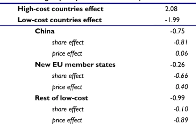
Overall, it is estimated that the increase in euro area import penetration from low-cost countries, whose share increased from over one third to more than a half since the start of the 2000s (see Chart 5) may have dampened euro area import prices of manufactures by about 2 percentage points each year between 1996-2007. This is mostly due to the “share effect” of China and the new EU Member Countries, which captures the downward impact on import prices of the rising import share of low-cost countries combined with the relatively lower price level of low-cost import suppliers. Meanwhile, the “price effect” – which captures the impact of export price inflation differentials between high and low-cost countries - makes a much smaller contribution to these downward pressures (See Table 1).15
Chart 5: Share of extra-euro area manufacturing imports from low-cost countries
(LHS: YoY change in percentage points; RHS: in %; quarterly data)
Table 1: Decomposition of euro area import prices (in %) 0 1 2 3 4 5 6 2001 2002 2003 2004 2005 2006 2007 2008 0 10 20 30 40 50 60
YoY change in percentage points (lhs) Share of low-cost count ries (rhs)
1996-2007 Manufacturing import price inflation in % p.a. 0.09
High-cost countries effect 2.08
Low-cost countries effect -1.99
China -0.75
share effect -0.81
price effect 0.06
New EU member states -0.26
share effect -0.66
price effect 0.40
Rest of low-cost -0.99
share effect -0.10
price effect -0.89
Source: Eurostat and ECB calculations; Table 1: Taglioni and Vergote (2009). Note: Last observation June 2008.
15
The methodology used in this analysis is described in detail in Appendix 1 and is similar to that of Kamin, Marazzi and Schindler (2004) who calculate the impact of the higher import share of China on US import price inflation. They find an average direct impact of China on US import inflation of around 1 percentage point per annum, which is somewhat higher but slightly below the estimates for the euro area.
Of course, as mentioned above, this is part of a relative price effect where inflation is simultaneously dampened from prices of imports of manufactured goods but accentuated by increases in other prices given global demand pressures (for example, Chart 5 above shows the strong rise in import prices of commodities related to strong emerging market economies’ demand for energy and other commodities such as metals and food). As relative price movements are a natural part of economic functioning and therefore need not necessarily have any effect on aggregate inflation, such movements may only be expected to have short-term aggregate inflationary impacts.
Apart from these direct relative price effects, globalisation may also put downward pressure on prices via increase competition in the labour and goods markets. Turning to recent euro area wage developments, globalisation may have been one contributing factor to an extended period of wage moderation within the euro area (for instance, if offshoring or the threat of offshoring reduces the wage demands of workers). For example, real wages have been weaker than productivity both on aggregate and also within the manufacturing and services (see Anderton and Hiebert, 2009, for an extended analysis of this issue). At the same time, there has been an ongoing weakening of the wage share for a longer period, which has been more severe than the corresponding fall in the US since the mid-80s, bringing this measure in both regions to historical lows (Chart 6). While such a development might be taken to indicate that the bargaining power of workers may have declined in the context of globalisation, extreme caution should be made in drawing such conclusions given several caveats related to measurement issues16 and the fact that much of this decline took place well before the recent phase of globalisation.17 As for globalisations impacts on prices, Pula and Skudelny (2009) use calculations based on several methodologies and find that a direct dampening effect of import openness on euro area producer price inflation of 0.1-1.0 percentage point for the euro area manufacturing sector over the
16It should be noted in this respect that several measurement problems limit the reliability of the wage share, including a growing importance of non-wage remuneration (particularly for the growing number of self employed), which imply that this measure cannot be interpreted reliably as the share of income accruing to capital or labour.
17
See Anderton and Hiebert (2009) for more details of globalisation’s possible impacts on the euro area labour market.
period 1996 to 2004. The authors report a dampening impact on euro area consumer price inflation of 0.05-0.2 percentage point per year on average based on aggregate data over the same period. Pain et al. (2006) find a combined effect on consumer inflation from lower non-commodity import price inflation and higher commodity import price inflation of up to 0.3 percentage point per annum over the period 2000 to 2005. Using similar methodologies, Chen et al. (2007) and Helbling et al. (2006), and Glatzer et al. (2006) report findings of a similar magnitude for other countries and regional groupings.
Chart 6: Long-term developments in labour shares
(in percentage of gross national income)
55 60 65 70 1960 1965 1970 1975 1980 1985 1990 1995 2000 2005 euro area United States
Source: Anderton and Hiebert (2009); AMECO database and ECB calculations.
Note: Self-employment adjusted labour shares; total domestic economy. The labour share is defined as the ratio of total compensation of employees to gross national income at current market prices.
3.4 Phillips Curves for the OECD economies
In this section, we look in more detail at the roles of unit labour costs, import prices, the output gap and monetary policy in the inflation process for the OECD economies. In particular, we see if the impact of the output gap on inflation changes over time as indicated in Section 2.2 and assess whether the relative roles of import prices and unit
labour costs in OECD inflation are changing, as well as evaluating how the inflation process might have changed due to monetary policy.
We estimate Phillips Curves based on a quarterly dataset ranging over the period 1970Q1-2008Q3, where we proxy the OECD by 9 individual OECD countries.18 The specification is based on a traditional backward-looking Phillips curve along the lines of previous work by, for example, Pain, Koske and Sollie (2006) and Eickmeier and Moll (2009):19 t j t i j j j t i j j t i j t i j j t i c p ygap ulc mp p
, seas 4 0 , 4 0 , , 4 1 ,where ptis the quarterly change in the log of the CPI, with the explanatory variables comprising the log of past inflation, the output gap (ygapi,t), log differences of quarterly total economy unit labor costs (ulci,t) and import prices of goods and services (mpi,t), as well as a constant (c) and seasonal dummies (seas).20 Subscript i relates to country i. As in previous papers, the output gap is only inserted for the current period without any lagged terms. A priori, we expect positive signs for the sums of the parameters of each of the explanatory variables.
This eclectic framework is a reduced form model similar to specifications estimated in various other empirical papers.21 The lagged inflation terms can be interpreted as representing the inflation expectations mechanism of economic agents based on information from past inflation, but also capture the dynamics of price adjustment and the degree of persistence of the inflation process which, in turn, are related to wage and price rigidities, institutional factors as well as monetary policy. Excess aggregate demand is captured by the output gap, while changes in import prices and unit labour
18
The 9 OECD countries are as follows: UK, USA, Sweden, Netherlands, Japan, Italy, France, Germany, and Australia.
19
Although forward-looking New Keynesian Phillips curve models have many advantages, it seems that backward-looking models may be more structurally stable in some respects (Stock and Watson, 2005), hence we prefer to estimate a backward-looking Phillips curve.
20
All data including the output gaps, unless otherwise stated, are obtained from the OECD Economic Outlook database.
21
See, for example, Lown and Rich (1997); Batini, Jackson and Nickell (2005); Borio and Filardo (2006); and Mody and Ohnsorge (2007), etc.
costs could be interpreted as supply-side influences or simply as other key additional factors affecting the inflation process.
We obtain panel estimates of the above equation by pooling the data across nine major OECD countries and thereby obtain a proxy for the parameters for the OECD as a whole. Therefore, in effect we impose the same slope parameters across different countries, but we include fixed effects so that each country has a different intercept. As the specification also includes lagged dependent variables, the estimators could be biased as the lagged dependent variable is correlated with the fixed effects.22 Consequently, the Arellano and Bond (1991) estimator based on GMM is frequently used in these circumstances. However, it is still correct to estimate the equation by Least Squares Dummy Variables (LSDV) as the LSDV estimator will still provide reasonable results in the present case as T is relatively large compared to N. 23 Another econometric issue is to test whether we can impose the same slope parameters across the different countries. A simple F-test shows that the restriction of equal slope parameters for each country is rejected.24 However, we note the assertion by Baltagi and Griffin (1983) that the empirical test of equal slope parameters in panel estimation can be frequently rejected despite the fact that there may be a strong economic rationale for imposing common slope parameters across the panel.
Our estimation strategy is to begin by estimating our basic Phillips’ Curve using different estimation techniques and comparing the results: first, we use the LSDV estimator; second, we check the LSDV results by estimating the same equation by GMM; third, given the rejection of the common slope restriction, we also estimate the equation using the Mean Group estimator which is the simple arithmetic average of the individual countries’ coefficients. We include 4 lags for each of the variables in
22
The bias results from the correlation between the lagged dependent variable and the transformed residuals. Nickell (1981) shows that the lagged dependent variable is biased towards zero, but that the bias decreases in T and disappears when T goes to infinity.
23
For example, Judson and Owen (1999) compare the bias of six different estimators of dynamic panel data models: the OLS estimator, the LSDV estimator, a corrected LSDV estimator as proposed by Kiviet (1995), two GMM estimators suggested by Arellano and Bond (1991), and the IV techniques used by Anderson and Hsiao (1981). Their findings are that the LSDV estimator performs just as well, or better than the majority of the alternatives as T increases and is larger than N. In addition, Kiviet (1995) notes that although the LSDV estimator is biased, its standard deviations are very small compared to different IV-estimators. Therefore, on the basis of the MSE-criterion (efficiency versus bias), Kiviet argues that LSDV may be preferable to alternative estimators.
24
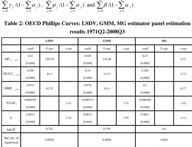
the above equation (with the exception that the output gap is only included for the current period but is also instrumented to avoid simultaneity problems).25 The results are shown in Table 2 below which reports the sum of the coefficients for each variable for which lags are included as well as an F-Test and P value of a Wald test that the parameters can be restricted to be zero.
The full sample results show that the signs of the variables are positive as expected while all key variables are statistically significant across all of the three estimation techniques (Table 2).26 Hence, past inflation, unit labour costs, import prices and the output gap are all significant determinants of inflation. The long-run parameters for ULC, MP and YGAP are respectively:
) 1 /( 4 1 4 0
j j j j , /(1 ) 4 1 4 0
j j j j and /(1 ) 4 1 4 0
j j j Table 2: OECD Phillips Curves: LSDV, GMM, MG estimator panel estimation results 1971Q2-2008Q3
coeff F-stat t-stat coeff F-stat t-stat coeff F-stat t-stat
0.61 0.649 0.47 [0.000] [0.000] [0.000] 0.209 0.16 0.299 [0.000] [0.000] [0.000] 0.079 0.079 0.1 [0.000] [0.000] [0.000] 0.000359 0.000373 0.000308 [0.000] [0.000] [0.000] 0.0014 0.0013 0.0011 [0.000] [0.003] [0.000] Adj-R2 Std. err. of regression LSDV GMM MG DPt-1,…,t-4 250.78 145.08 8.31 DULCt,…,t-4 44.4 14.74 4.72 DMPt,…,t-4 62.75 45.4 6.77 YGAP t 3.41 3.31 1.82 C 3.54 2.95 4.13 0.762 0.759 0.6 0.0058 0.0058 0.004
Notes: F-tests relate to exclusion tests of the parameters (p-values in square brackets); unbalanced panel; country specific fixed effects included; seasonal dummies included; LSDV=Least Squares Dummy Variables estimated by instrumental variables (YGAP instrumented by own lagged values); GMM=Arellano and Bond Generalised Method of Moments; MG=Mean Group Estimator.
25
The output gap is instrumented by its own lagged values. 26
The F-tests decisively reject the null hypothesis that the sum of the coefficients are zero for lagged inflation, unit labour costs and import prices.
Overall, the results generally tend to be very similar across the three techniques, with the LSDV and GMM results particularly close to each other. Meanwhile, the MG estimator results are also similar except that the sum of the lagged inflation parameters tend to be somewhat smaller, and the sum of the unit labour cost parameters larger, in comparison to the results for the other two estimators. In addition, the output gap term is less significant when using the MG estimator. In terms of the long-run parameters, the LSDV results show that the relative weights of ULC and MP are around two thirds and one third respectively (ie, long-run parameters of about 0.54 and 0.21 respectively).27
.
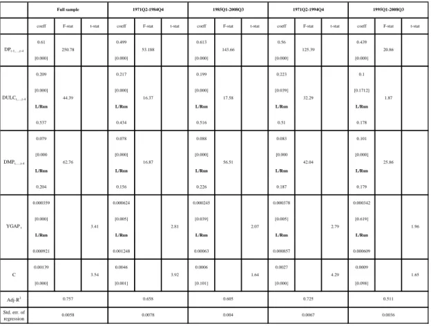
Our next step is to see if there is any break in the parameters over time – which may be due to factors such as globalisation, etc - by estimating the equations over different sample periods. Based on rolling-window parameter estimates and other information, we chose two possible periods for structural breaks: first, from 1985 onwards; second, from 1995 onwards.28 The results are reported in Table 3. However, given the similarity of the full sample period results across the three different techniques, we only report the results for the LSDV estimator (although we also describe in the text the results of the other techniques if they differ from the LSDV estimator).
Some key results of the split period analysis reported in Table 3 are as follows:
There seems to be some evidence that the long-run output gap parameter becomes smaller in magnitude over time: the results for the period 85Q1-08Q3 show that the long-run YGAP parameter is about half the size of the earlier period, while for the 95Q1-08Q3 sample it is about two-thirds the magnitude of the previous period. In addition, the MG-estimator results point to a stronger conclusion as they show that the output gap parameter is not
27
The parameters are very similar in magnitude to those of Pain et al (2006) as well as Eickmeier and Moll (2009).
28
The break from 1985 onwards also corresponds to Charts 2a,b on the relationship between euro area inflation and the output gap; while a break from 1995 onwards also corresponds to period of increased globalisation when countries such as China and those from previously communist eastern Europe started to become more integrated in the world economy. The 1995 break is also similar to that found statistically significant by Pain et al (2006).
statistically significant in the most recent period.29 Overall, the general result of a weaker impact of the output gap on inflation in the most recent period seems to be in line the anecdotal evidence as well as some hypotheses related to globalisation as discussed in Section 2.2.
The results for the period 95Q1-08Q3 also seem to indicate: (i) a decline in the persistence of inflation (ie, the estimated sum of lagged dependent variable parameters declines from 0.56 during 71Q2-94Q4 to 0.44 in the period 95Q1-08Q3). This corresponds with various other studies that find that the degree of inflation persistence has declined over time and may be related to improvements in monetary policy;30 (ii) an increase in the long-run parameter for import prices relative to unit labour costs.31 This is consistent with the fact that the degree of import penetration has increased over time - as measured by imports as a percentage of GDP - and therefore automatically has an increasing weight in the determination of inflation.32
29
The t-statistics for the output gap (YGAP) parameter using the MG-estimator for the periods 1985Q1-2008Q3 and 1995Q1-2008Q3 are 0.801 and 0.256 respectively.
30
Declines in inflation persistence over time may also be associated with increased credibility of monetary policy and movements towards better well-anchored inflation expectations (see, for example: Alogoskoufis, 1992; Anderton, 1997). Hence, these results are also consistent with the GVAR simulation results in Section 3.2 which claims that oil price shocks do not feed through to core inflation because of well-anchored inflation expectations.
31
The size of the import price parameter also increases relative to the unit labour costs parameter for the 85Q1-08Q3 period.
32
However, the increase in magnitude of the import price parameter may also be due to an increase in international competition – particularly due to rising imports from low-cots countries – which can also put additional downward pressure on inflation.
Table 3: OECD Phillips’ Curves: LSDV Panel estimation results over different sample periods
coeff F-stat t-stat coeff F-stat t-stat coeff F-stat t-stat coeff F-stat t-stat coeff F-stat t-stat
0.61 0.499 0.613 0.56 0.439
[0.000] [0.000] [0.000] [0.000] [0.000]
0.209 0.217 0.199 0.223 0.1
[0.000] [0.000] [0.000] [0.039] [0.1712]
L/Run L/Run L/Run L/Run L/Run
0.537 0.434 0.516 0.51 0.178
0.079 0.078 0.088 0.083 0.101
[0.000 [0.000] [0.000] [0.000 [0.000]
L/Run L/Run L/Run L/Run L/Run
0.204 0.156 0.226 0.187 0.179
0.000359 0.000624 0.000245 0.000378 0.000342
[0.000] [0.005] [0.039] [0.005] [0.619]
L/Run L/Run L/Run L/Run L/Run
0.000921 0.001248 0.00063 0.000857 0.000609 0.00139 0.0046 0.0006 0.0027 0.0009 [0.000] [0.001] [0.101] [0.000] [0.098] Adj-R2 Std. err. of regression 0.0058 0.0078 0.004 0.0067 0.0036 1.65 0.757 0.658 0.605 0.725 0.511 1.96 C 3.54 3.92 1.64 4.29 YGAP t 3.41 2.81 2.07 2.79 DMPt,…,t-4 62.76 16.87 56.51 42.04 17.58 32.29 DULCt,…,t-4 44.39 16.37 1995Q1-2008Q3 DPt-1,…,t-4 Full sample 1971Q2-1984Q4 1985Q1-2008Q3 1971Q2-1994Q4 250.78 53.188 143.66 125.39 20.86 1.87 25.86
Notes: Panel estimates based on Least Squares Dummy Variables (LSDV) results estimated by instrumental variables (YGAP instrumented by own lagged values); F-tests relate to exclusion tests of the parameters; unbalanced panel; country specific fixed effects and seasonal dummies included.
3.5 Global components of inflation
A related aspect to the above mechanisms is that the global component of inflation seems to have increased in size relative to domestic component (see Eickmeier, 2008; Neely and Rapach, 2009). Although further analysis on this issue is beyond the scope of this paper, it is worthwhile to summarise the contrasting evidence that domestic inflation has become more sensitive to measures of foreign slack in addition to the standard import price channel.33 On the one hand, Borio and Filardo (2007) find a significant role for global economic slack measures in Phillips Curves of advanced economies (albeit with mixed results for the euro area). Studies such as Paloviita (2007) and Rumler (2007) find euro area inflation dynamics are better captured by an open economy specification. In a similar vein, Ciccarelli and Mojon (2005) find that
33 Globalisation may have weakened the link of domestic liquidity on domestic prices or, alternatively, implied a higher role for
foreign liquidity in domestic prices; Rueffer and Stracca (2006) find that evidence of a significant spill-over of global liquidity to the euro area economy.
for several OECD countries, the global inflation rate moves largely in response to global real variables over short horizons and global monetary variables at longer horizons. In looking at inflation dynamics of highly disaggregated consumer price data, Monacelli and Sala (2007) find that a sizeable fraction of the variance of inflation explained by macroeconomic factors attributable to "international" factors for both Germany and France, but that such factors are more relevant in the goods/manufacturing sector than in the service sector. For the UK, Batini et al (2005) find external competitive pressures also seem to affect U.K. inflation via their impact on the equilibrium price markup of domestic firms. On the other hand, many other studies have failed to identify a significant role for global economic slack measures in Phillips Curves of advanced economies. Specifically for the euro area, Calza (2008) finds limited evidence in support of the “global output gap hypothesis”. Indeed, Musso et al. (2007) find that a flattening of the slope of the euro area Phillips curve occurred mainly in the 1980s, before the current globalisation phase. Meanwhile, Ball (2006), Woodford (2007), Ihrig et al. (2007) and Wynne and Kersting (2007) argue for a negligible role for measures of global economic slack on inflation dynamics, while Pain et al. (2006) relate a rise in the sensitivity to domestic inflation in OECD economies to foreign economic conditions to an import price channel alone. On the basis of a new Keynesian Phillips curve-based model, Sbordone (2008) finds it difficult to argue that an increase in trade would have generated a sufficiently large increase in U.S. market competition to reduce the slope of the inflation-marginal cost relation.
4. Conclusions
Against the background of large fluctuations in world commodity prices and world growth, combined with ongoing structural changes relating to globalization, this paper assesses some of the key elements of global inflation. The paper considers various relative price and structural impacts on global inflation by: estimating a GVAR to examine how oil price shocks feed through to core and headline inflation; calculating the impact of increased imports from low-cost countries on manufacturing import prices; estimating Phillips curves in order to shed light on whether the inflationary
process in the OECD countries has changed over time, particularly with respect to the roles of import prices, unit labour costs and output gaps.
The first part of the paper provides the relevant background to the analysis by looking at longer-term as well as current trends in global inflation. We document how OECD inflation has fallen dramatically since the 1970s and look at more recent inflation developments, particularly in the context of the rise in oil and other commodity prices since the start of the 2000s.
The second part of the paper investigates the role of ongoing structural factors and relative price shocks in the global inflationary process. On the import prices side, globalisation forces seem to have had a dampening effect on inflation until the mid-2000s associated with low prices of imports of manufactured goods through increased global supply of goods and labour from low-cost countries which, more recently, may have been offset by strong increases in the prices of commodities such as oil (until the first half of 2008) resulting from heightened global demand pressures. At the same time, international competitive pressures may have also contributed to reducing inflationary pressures in the OECD economies via wage moderation and lower growth of unit labour costs. Meanwhile, the GVAR simulations – based on past recent behaviour in the 2000s - suggest that oil price shocks may not have significant (or very limited) impacts on core inflation in the euro area and US (assuming responses are linear and symmetric regarding the magnitude and sign of oil price shocks), possibly via the reduction of second-round effects due to well-anchored inflation expectations in containing inflationary pressures. Finally, over a longer time scale, estimated Phillips curves for the OECD economies provide some tentative evidence that the impact of the output gap on the inflation of OECD economies may be becoming weaker over time, possibly due to effects from globalisation and/or changes in monetary policy. By contrast, import prices seem to be growing in importance in the inflation process - in line with their increasing weight in the CPI - while the persistence of inflation seems to be declining which may be related to changes in monetary policy associated with lower and well-anchored inflation expectations.
Appendix 1: Methodology used for calculating impacts of low-cost
countries on the euro area’s manufacturing import price.
In order to decompose the changes in the euro area manufacturing import unit value into the effects arising from a change in the geographical distribution of imports between high-cost and low-cost countries (and among them, CN, NMS and ROLC34), two factors have to be considered separately: a share effect (what would have been observed if only the share changed), and a price effect (what would have been observed if only the import price from low-cost countries had changed relative to that of the high-cost countries).
The methodology used to decompose import price inflation
As the euro area absolute import unit value is a weighted average of the import unit values from various countries of provenance, the percentage change in the euro area import unit value from period t-n to period t can be deduced from equation (4), which takes into consideration the fact that the sum of the weights adds to 1, and sets the group of high-cost countries as the reference point:
n t n t HC n t HC t HC j j t n n t HC n t HC t HC n t n t j n t j t j n t j t j n t t HC t j n t t p p p p p p p p p p p p p p p p p
, , , , , , , , , , , , ,
CN NMS ROLC
j , , (1) .In equation (1), for each low-cost country j, the first and second terms capture the direct effect of imports from that country on the change in the euro area import price:
The first term is the share effect – that is, the effect of a change in the import share from a particular country given its price differential against the reference (high-cost) group of countries. If the country’s import price is lower than that of the reference country, then an increase in its import share will change the composition of imports towards cheaper goods and will therefore have a negative effect on the overall import price. The size of the share effect depends on both the magnitude of the change in the share, and the import price differential of country j against the reference country.
The second term in the equation represents the price effect. It captures the change in the euro area import price due to different import price inflation rates for country j and the reference country. If the import price from country j
increases by more (decreases by less) than that of the reference country, then given the geographical composition of imports, the country will have a positive
34
(negative) impact on the overall euro area import price. The impact increases with the import share of country j.
Finally, the third term in the decomposition represents the residual effect due to price developments in the high-cost countries.
The caveats of the methodology
The methodology employed in the note is subject to four main caveats:
Firstly, the aggregate euro area import unit value series computed is slightly different from the unit value series officially published by Eurostat. The differences arise mainly due to methodological differences in the aggregation. In contrast to the computed unit value series, the officially published one is based on Fischer index.
Secondly, the results of the magnitude of the share and price effects depend on the grouping of the countries, and therefore on the reference country. As this note focuses on the effect of imports from the low-cost countries, the results are decomposed into China, the NMS and ROLC, whereas the high-cost countries remain aggregated and represent the reference point. However, it should be noted that if the aim were to analyse the effects of imports from just one country vis-à-vis all other import partners, the results would be different. For example, if the focus were purely on Chinese imports, the share effect of China against the rest of the import partners would be lower than that against just the high-cost countries. This is so because the difference between the import price level of China and that of the rest of the world would be lower than with that of high-cost countries. The price effect would also be affected, although it is not possible to know a priori in which direction.
Thirdly, when setting the high-cost countries as the reference, it is implicitly assumed that the low-cost countries (countries with linearly independent weights in the aggregation) are competing against the high-cost countries, but not among themselves. So by construction, an increase in country j’s import share is thus always a substitution for imports from the high-cost countries, but not for imports from the NMS or any other low-cost country or country group.
Finally, import shares in value terms are used for the aggregation of the import unit value, thus in addition to structural developments also capturing valuation effects. The available alternative would be to use import share in volume terms. However, Eurostat Comext database reports volumes measured in weight units (multiples of kilograms) that are difficult to interpret at an aggregate level.
References:
Amiti M and D Davis (2009), “What’s Behind Volatile Import Prices from China?”, Federal Reserve Bank of New York Current Issues in Economics and Finance, Volume 15, Number 1 (January).
Alogoskoufis, G. (1992), “Monetary accommodation, exchange rate regimes and inflation persistence”, Economic Journal 102 (May), pp. 461-480.
Anderton, R. (1997), “Did the Underlying behaviour of inflation change in the 1980s? A Study of 17 countries”, Welwirtschaftliches Archiv, Band 133, Heft 1, pp. 22-38.
Anderton, R., di Mauro, F. and Moneta, F. (2004), “Understanding the impact of the external dimension on the euro area: trade, capital flows and other international macroeconomic linkages”, European Central Bank Occasional Paper no. 12.
Anderton, R., Brenton, P. and Whalley. J. (2006) Globalisation and the Labour Market: Trade, Technology and Less-Skilled Workers in Europe and the United States
(2006: Routledge, London) edited by Robert Anderton, Paul Brenton and John Whalley.
Anderton, R. and di Mauro, F. (2007), “The external dimension of the euro area: stylised facts and initial findings” in The External Dimension of the Euro Area:Assessing the Linkages”, edited by F. di Mauro and R. Anderton, Cambridge University Press, London.
Anderton, R. and Kenny, G. (2009) forthcoming Globalisation and Macroeconomic Performance, Cambridge University Press.
Anderton. R. and Hiebert, P. (2009) “The impact of globalisation on the euro area macroeconomy”, University of Nottingham Globalisation and Economic Policy Research Paper no. 2009/14.
Anzuini, A., Pagano, P. and Pisani, M. (2007), “Oil supply news in a VAR: information from financial markets”, Banca D’Italia Working Paper no. 632.
Arellano, M. and Bond, S. (1991), “Some tests of specification for panel data: Monte Carlo evidence and an application to employment equations”, Review of Economic Studies, Vol. 58, pp. 277-297.
Baltagi, B. and Griffin, J. (1983), “Gasoline demand in the OECD: An application of pooling and testing procedures”, European Economic Review, 22, pp. 117-137. Batini,N., Jackson, B. and Nickell, S. (2005), “An open-economy new Keynesian Phillips Curve for the UK”, Journal of Monetary Economics, vol. 52 (6), pp. 1061-1071.
Ball L (2006), “Has globalisation changed inflation?”, NBER Working Paper No. 12687 (November).
Bean C (2007), “Globalisation and inflation”, Bank of England Quarterly Bulletin 2006Q4. Bickel, P. and Buhlman, P. (1997), “A new mixing notion and functional central limit theorems for a Sieve bootstrap in time series”, Bernoulli, 5(3), 413-446.
Borio C and A Filardo (2007), “Globalisation and inflation: New cross-country evidence on the global determinants of domestic inflation”, Bank for International Settlements Working Paper No. 227 (May).
Blanchard, O.J. and Gali, J. (2007), “The macroeconomic effects of oil price shocks: why are the 2000s so different from the 1970s”, NBER Working Paper no. 13368, September.
Buhlman, P. (1997), “Sieve bootstrap for time series”, Bernoulli, 3 (2), 123-148.
Calza, A. (2008), “Globalisation, domestic inflation and global output gaps: Evidence from the euro area”, ECB Working Paper No. 890.
Cecchetti, S. and Moessner, R. (2008), “Commodity prices and inflation dynamics”, BIS Quarterly Review, December 2008.
Ciccarelli, M and B Mojon (2005): “Global inflation”, ECB Working Paper Series, No 537, also forthcoming in Review of Economics and Statistics.
Dees, S., di Mauro, F., Pesaran, M.H. and Smith, L.V. (2007), “Exploring the international linkages of the euro area: a global VAR analysis”, Journal of Applied Econometrics, 22 (1), 1-38.
Dees, S., Karadeloglou, P. Kaufmann, R.K. and Sanchez, M. (2007), “Modelling the world oil market: assessment of a quarterly econometric model”, in Energy Policy, Vol. 35, No. 1, 2007, pp. 178-191.
ECB (2008), “Globalisation, Trade and the Euro Area Macroeconomy,” ECB Monthly Bulletin (January).
ECB (2006b), “Effects of the rising integration of low-cost countries on euro area import prices,” in Monthly Bulletin, August.
ECB (2009a), “Expectations and the conduct of monetary policy”, Monthly Bulletin, May. Eickmeier, S. and Moll, K. (2008): “The Global Dimension of Inflation – Evidence from Factor-Augmented Phillips Curves”, ECB Working Paper Series, No 1011
Feenstra R (2007), “Globalisation and Its Impact on Labor,” Global Economy Lecture, Vienna Institute for International Economic Studies (February).
Galesi, A. and Lombardi, M. (2008), “External shocks and international inflation linkages: a Global VAR analysis”, Paper presented at the University of Cambridge 1st Macroeconomics and Finance Conference, November 2008.
Glatzer E, E Gnan and M Valderrama (2007), “Globalisation, Import Prices and Producer Prices in Austria,” Oesterreische Nationalbank Monetary Policy & the Economy Q3/06.