Comparative Study of
1
D De-noising Techniques
Using Induction Motor Fault Signals
This Thesis is submitted in partial fulfillment of the requirement for the degree of
Bachelor of Computer Science and Engineering
Under the Supervision of
Dr. Jia Uddin
By
Rehnuma Tasnim Lamia(10201012)
Zafor Iqbal (14341015)
School of Engineering and Computer Science
August 2016
BRAC University, Dhaka, Bangladesh.
Comparative Study of
1
D De-noising Techniques
Using Induction Motor Fault Signals
This Thesis is submitted in partial fulfillment of the requirement for the degree of
Bachelor of Computer Science and Engineering
Under the Supervision of
Dr. Jia Uddin
By
Rehnuma Tasnim Lamia(10201012)
Zafor Iqbal (14341015)
School of Engineering and Computer Science
August 2016
I
DECLARATION
We, hereby declare that this thesis is based on the results found by our own task. Materials of work found by other researcher are mentioned by reference. This Thesis, neither in whole or in part, has been previously submitted to any other University or any Institute for the award of any degree or diploma.
Signature of Supervisor Signature of Author
Dr. Jia Uddin Rehnuma Tasnim Lamia
II
ACKNOWLEDGEMENTS
All thanks to Almighty ALLAH, the creator and the owner of this universe, the most merciful, beneficent and the most gracious, who provided us guidance, strength and abilities to complete this research.
We are especially thankful to Dr. Jia Uddin, our thesis supervisor, for his help, guidance and support in completion of my project. We also thankful to the BRAC University Faculty Staffs of the Computer and Communication Engineering, who have been a light of guidance for us in the whole study period at BRAC University, particularly in building our base in education and enhancing our knowledge.
Finally, we would like to express our sincere gratefulness to our beloved parents, brothers and sisters for their love and care. We are grateful to all of our friends who helped us directly or indirectly to complete our thesis.
III
CONTENTS
DECLARATION………. I ACKNOWLEDGEMENTS……… II CONTENTS………….………... III LIST OF FIGURES………. VI LIST OF TABLES………... VIII LIST OF ABBRIVIATIONS…….………. IXABSTRACT………. 1
CHAPTER I: INTRODUCTION………... 2
1.1 Motivations………. 2
1.2 Induction Motor Fault Signals……… 3
1.2.1. Rotor faults………. 3
1.2.2. Short turn faults……….. 3
1.2.3. Air gape electricity………. 4
1.2.4. Bearing faults………. 4
1.3 Contribution Summary……… 4
1.4 Thesis Orientation………... 5
CHAPTERII: BACKGROUND INFORMATION………. 6
2.1 1-D Signal Overview……….. 6
2.2De-noising………... 6
2.3 Related Work in 1D De-noising Techniques……….. 6
CHAPTER III: RESEARCH METHODS AND SPECIFICATIONS……… 8
3.1 Parameters Overview……….. 8
3.1.1 Mean Squared Error……… 8
3.1.2 Root Mean Square Error………. 8
IV
3.1.4 Signal to Noise Ratio……….. 9
3.1.5 Peak Signal to Noise Ratio……….. 9
3.1.6 Cross Correlation……… 10
3.1.7 Structural Similarity……… 10
3.1.8 Structural Dissimilarity………... 11
3.2 Research Methods Overview……….. 11
3.2.1 Butter Worth……… 11
3.2.2 Low Pass Filter……… 11
3.2.3 High Pass Filter………... 12
3.2.4 Band Stop Filter……….. 13
3.2.5 Median Filter………... 13
3.2.6 Hilbert Filter……… 13
3.2.7 Discrete Wavelet Transform (DWT)………. 14
3.2.8 Empirical Mode Decomposition (EMD)……… 14
3.2.9 Gabor Filter………. 14
3.2.10 Q Function………. 15
CHAPTER IV: EXPERIMENTAL SETUP ………..…..…..….. 16
4.1 Architecture Overview……… 16
4.2 ArchitectureDescription ……….... 17
4.2.1 Input……… 17
4.2.2 De-noising………... 18
4.2.3 Performance Analysis………. 19
CHAPTER V: EXPERIMENTAL RESULT ANALYSIS………...…...…. 20
5.1 Implementation………... 20
5.2 Output Signal Analysis………... 20
5.2.1 Butter Worth……… 21
V
5.2.3 High Pass Filter………... 23
5.2.4 Band Stop Filter……….. 24
5.2.5 Median Filter………... 25
5.2.6 Hilbert Filter……… 26
5.2.7 Discrete Wavelet Transform (DWT)………. 27
5.2.8 Empirical Mode Decomposition(EMD)……… 27
5.2.9 Gabor Filter………. 31
5.2.10 Q Function………. 32
5.3 Parameter Value Analysis………... 33
5.4 Parameter Value Comparison………. 34
5.4.1 Mean Squared Error……… 34
5.4.2 Root Mean Square Error………. 35
5.4.3: Mean Absolute Error……….. 36
5.4.4 Signal to Noise Ratio……….. 37
5.4.5 Peak Signal to Noise Ratio………... 38
5.4.6 Cross Correlation………. 39
5.4.7 Structural Similarity……….. 40
5.4.8 Structural Dissimilarity………... 41
CHAPTER VI: CONCLUSIONS AND FUTURE WORKS………... 42
6.1 Concluding Remarks………... 42
6.2 Future Works………... 42
VI
LIST OF FIGURES
Figure 1: Statistics of different faults in an induction motor 3 Figure 2: Experimental architecture for 1d de-noising techniques 16 Figure 3: 1D Input Signal of Induction Motor 18
Figure 4: De-noised Signal 18
Figure 5: Performance Analysis Technique 19 Figure 6: Generated Signal of Butter Worth 21 Figure 7: Closer Look of Generated Signal of Butter Worth 21 Figure 8: Generated Signal of Low Pass Filter 22 Figure 9: Closer Look of Generated Signal of Low Pass Filter 22 Figure 10 Generated Signal of High Pass Filter 23 Figure 11: Closer Look of Generated Signal of High Pass Filter 23 Figure 12: Generated Signal of Band Stop Filter 24 Figure 13: Closer Look of Generated Signal of Band Stop Filter 24 Figure 14: Generated Signal of Median Filter 25 Figure 15: Closer Look of Generated Signal of Median Filter 25 Figure 16: Generated Signal of Hilbert Filter 26 Figure 17: Closer Look of Generated Signal of Hilbert Filter 26 Figure 18: Generated Signal of DWT Algorithm and Original Signal (Red) 27 Figure 19: IMF 1 residue, iteration before and after 28 Figure 20: IMF 2 residue, iteration before and after 28 Figure 21: IMF 3 residue, iteration before and after 28 Figure 22: IMF 4 residue, iteration before and after 29 Figure 23: IMF 5 residue, iteration before and after 29 Figure 24: IMF 6 residue, iteration before and after 29 Figure 25: IMF 7 residue, iteration before and after 30 Figure 26: Generated Signal of EMD Algorithm 30 Figure 27: Generated Signal of Gabor Filter 31 Figure 28: Closer Look of Generated Signal of Gabor Filter 31 Figure 29: Generated Signal of Q Function 32 Figure 30: Closer Look of Generated Signal of Q Function 32 Figure 31: Mean Squared Error comparison in different parameters 34 Figure 32: Mean Squared Error parameter values 34 Figure 33: Root Mean Square Error comparison in different parameters 35
VII
Figure 34: Root Mean Square Error parameter values 35 Figure 35: Mean Absolute Error comparison in different parameters 36 Figure 36: Mean Absolute Error parameter values 36 Figure 37: Signal to Noise Ratio comparison in different parameters 37 Figure 38: Signal to Noise Ratio parameter values 37 Figure 39: Peak Signal to Noise Ratio comparison in different parameters 38 Figure 40: Peak Signal to Noise Ratio parameter values 38 Figure 41: Cross Correlation comparison in different parameters 39 Figure 42: Cross Correlation parameter values 39 Figure 43: Structural Similarity comparison in different parameters 40 Figure 44: Structural Similarity parameter values 40 Figure 45: Structural Dissimilarity comparison in different parameters 41 Figure 46: Structural Dissimilarity parameter values 41
VIII
LIST OF TABLES
Table 01: Parameter Values of MSE, RMSE, MAE, SNR 33
IX
LIST OF ABBREVIATIONS
1-D One Dimensional MSE Mean Squared Error RMSE Root Mean Squared Error MAE Mean Absolute Error SNR Signal-to-Noise-Ratio PSNR Peak-Signal-to-Noise-Ratio CC Cross Correlation
SSIM Structural Similarity DSSIM Structural Dissimilarity DWT Discrete Wavelet Transform EMD Empirical Mode Decomposition BW Butter Worth
1
ABSTRACT
Removing noise from the original signals has always been challenging. A lot of de-noising techniques and algorithms has already been published and are being used now-a-days. But knowing which de-noising method is better we need to compare the performance of their applications so that a new group of people can start working instantly knowing which method is better than the other considering specific parameters.
In this thesis, we will compare the de-noising techniques using discrete wavelet transform (DWT), empirical mode decomposition (EMD), Gabor filter, butter filter, low pass filter, high pass filter, band stop filter, Hilbert filter, Median filter and Q function. To evaluate the performance of the state-of-art models we will utilize an induction motor dataset that consist of inner, outer, and roller fault signals including healthy/normal signal. Finally, the performance will be measured using the following parameters: signal to noise ratio (SNR), peak signal to noise ratio (PSNR), mean square error (MSE), root mean square error (RMSE) and mean absolute error (MAE). We will also find the structural similarity(SSIM), structural dissimilarity(DSSIM) and cross correlation (CC) between the parameter.
2
CHAPTER I
INTRODUCTION
1.1. MotivationsInduction motor is an important component in many industrial fields as it is generally incorporated in profitable equipment, such as conveyor belts, pumps, air compressors etc.It is one of the widely used machines in industry due to their ruggedness and flexibility. However, different types of electrical and mechanical faults can occur due to heavy duty cycles, poor working environment, and installation, which prevent the normal working atmosphere of it [1]. Bearing is a major part of the induction motor, which plays a very significant role in industrial applications. Therefore, its malfunction in the practical operation can lead to the breakdown of whole machine. In general, several faults could occur on different parts of induction motors after running a long time, such as rotor (10%), stator (38%), bearing (40%), or other parts (12%) [2]. They will hamper directly in the manufacturing process of the factory by expensive machine downtime, renovating and replacing cost, indirectly effect to the product quality and dealer prestige. Therefore, the fault diagnosing system has become a vital contribution in handling with faulty trouble of the induction motor; it benefits to identify any abnormal indication of machine successively and informs the authority to resolve the matter in time.
However, many methods have been proposed for fault detection and diagnosis, but most of the methods require a good deal of expertise to apply them fruitfully. Simpler approaches are needed to enable even incompetent operators with actual knowledge of the system to scan the fault condition and make reliable decisions. To satisfy our goal we can use some one-dimensional de-noising techniques. We will utilize inner faults signals as an input signal using different parameter for measuring the performance as well as getting the structural similarity and dissimilarity between the parameters.
3
Figure 1: Statistics of different faults in an induction motor [2].
1.2. Induction Motor Faults Signal
The common internal faults of induction motor are short turn winding fault, rotor faults, bearing faults, gear fault and misalignment. The common internal fault can be two types [3].
Electrical faults Mechanical faults
Winding insulation problem causes Electrical faults which can be defined by rotor faults on the other hand bearing faults, load faults and misalignment of shaft are categorize by Mechanical faults [3].
1.2.1. Rotor faults
Usually, Lower grade machine are made of die casting techniques where as high grade machine is made of copper rotor bar. Technological difficulties can be occurred for the consequences of melting bars and end rings. As a result, induction motor shows irregular in the rotor [3].
1.2.2. Short turn faults
35-40% failure of induction motor causes due to the stator winding insulation [4]. A large percentage of winding connected failure are originated by insulation failure of more than a few turns of a stator coil inside one phase. This type of faults is denoted by short turn faults [5]. 40% 38% 10% 12% Bearing Stator Rotor Other Parts
4 1.2.3. Air gape electricity
It is a common rotor fault of induction motor. It creates some vibration and noise. In a high grade machine, the rotor is center-aligned with the stator bore as the rotor‟s center of rotation is equivalent to the geometric center of the stator bore [6,7]. When the rotor is not the centered aligned, the unbalanced radical pressure can be the reason of a stator-to- rotor rub which can destruction to the stator and the rotor [8, 9].
1.2.4. Bearing faults
Bearing are common elements of electrical machine. 40% of the of machine failure happen due to bearing faults [1]. Bearing contains two ring named inner and outer rings. A set of balls or rolling elements located in the channels of rotating rings. A continue pressure on the bearing causes exhaustion failure usually at the inner and outer races of the bearings. This failure produces measurable vibration and raises the level of the noise.
1.3 Contribution Summary
The summary of the main contributions is as follows:
Eliminating noise from the original signals and measuring the output has always been very tricky. A lot of de-noising techniques and algorithms are available and being used now-a-days. But at the same time knowing which de-noising method is healthier than other methods, we need to compare the performance of their applications.
We will compare the de-noising techniques which are Discrete Wavelet Transform (DWT), Empirical Mode Decomposition (EMD), Gabor filter, butter worth filter, low pass filter, high pass filter, band stop filter, Hilbert filter and Median filter.
To estimate the performance of the state-of-art models we will operate an induction motor dataset that consists of inner faults.
Finally, the performance will be measured using the following parameters: Signal to Noise Ratio (SNR), Peak Signal to Noise Ratio (PSNR), Mean Square Error (MSE), Root Mean Square Error (RMSE), Cross Correlation(CC) and Q function. We will also find the Structural Similarity (SSIM) and Structural Sissimilarity (DSSIM) between the parameter.
5 1.4 Thesis Orientation
The rest of the thesis is organized as follows:
CHAPTER II includes the necessary background information regarding the methods we applied to get our outputs.
CHAPTER III includes the research methods and specifications that are crucial for developing our experimental architecture.
CHAPTER IV describes the experimental setup of the denoising technique. CHAPTER Vdemonstrates the experimental result analysis
6
CHAPTER II
BACKGROUND INFORMATION
2.1 1D Signal OverviewIn physics and mathematics, a sequence of n numbers can be understood as a location in n-dimensional space. When n = 1, the set of all such locations is called a one-dimensional space. In general image processing 1D, 2D and 3D images are used. 1D signal are treated as matrix with numerous number of rows with a single column values. People usually take individual rows from images to be used as 1D signals.
In signal processing, a 1D signal is a line graph through the entire sample. Peaks in the spectra correspond to a given value in the sample. This can allow the researcher to identify specific behavior of machine on certain conditions. Let‟s consider a 1D signal of audio from any machine as an example to see what the different domains of signal mean. At first, it can be sampled the amplitude of the sound many times a second, which gives an approximation to the sound as a function of time. Then we will analyses the sound in terms of the pitches of the notes, or frequencies, which make the sound up, recording the amplitude of each frequency. In our thesis we use the same approach as described where we sample the output or de-noised signal and analyze them according to our predefined parameters.
2.2 De-noising
De-noising is the extraction of a signal from a mixture of signal and noise. De-noising can also be defined as the process with which we reconstruct a signal from a noisy one. The presence of noise in signal restricts one‟s ability to collect meaningful information. Noise in experimental data will result in incorrect output which will result in misleading conclusions [11].
2.3 Related Work in 1D De-noising Techniques
The main objective of a fault de-noising system is to diagnose any symptom of faults. It could be very important in industrial processes of any manufactory since the predicted faults step can create some proofs to provide adequate warning of imminent failures. It also helps to schedule future preventative maintenance and prepare the necessary spare parts for the considering devices before strip down [12]. De-noising using different methods and parameter has been applied by different literature [12-16]. Reliable Fault Diagnosis of Induction Motors using an Acoustic Emission Sensor and Signal Processing Techniques [12] proposes a reliable fault diagnosis approach of induction motors using an acoustic emission (AE) sensor and signal processing techniques.
7
In the proposed approach, discrete wavelet transform (DWT) is utilized to decompose the AE signal and select the appropriate nodes using the maximum energy ratio (MER). Then, a one-dimensional (1D) Gabor filter with various frequencies and orientation angles is applied to reduce the abnormalities and extract a number of statistical parameters.
Rolling Bearing Fault Diagnosis based on Time-frequency Feature Parameters and Wavelet Neural Network [13] proposes a novel method in fault diagnosis of rolling bearing based on time-frequency feature parameters and wavelet neural network. First, the time feature parameters are extracted from the vibration signal.
Then the empirical mode decomposition (EMD) is used to decompose the signals of rolling bearings into a number of intrinsic mode functions (IMFs), and then the IMF energy-torques could be calculated through the vibration signal. Finally, those time-frequency feature parameters are taken as fault samples to train wavelet neural network (WNN).
In the previous paper researcher have used two or three methods and parameters but in our thesis we have used ten methods and eight parameters at a time to get to our concluding remarks. The many methods and parameters will give us a clear view of which method is better considering the other ones while de-noising 1d signals. This research paves the way to work with more similar methods and find out the better ones considering different data set of induction motor.
8
CHAPTER III
RESEARCH METHODS AND SPECIFICATIONS
In this chapter, we will describe the parameters that are needed for performance analysis of the 1D-output signal. Moreover, the algorithms or methods which are used in de-noising technique are presented thoroughly here.
3.1 Parameters Overview
In the phase of performance analysis, we have used eight different types of parameters for signal analyzing. The eight parameters are Mean Squared Error, Root Mean Square Error, Mean Absolute Error, Signal to Noise Ratio, Peak Signal to Noise Ratio, Cross Correlation, Structural Similarity, Structural Dissimilarity. The performance parameters are described in given order.
3.1.1 Mean Square Error
Mean Square Error is a dominant quantitative performance metric in the field of signal denoising. It is used for the assesment of signal quality and fidelity. The cumulative squared error that occurs between noisy and original form of image is termed as MSE. It is mathematically defined as[17]:
MSE =
∑ ∑ ) ))
(1) where m is the number of rows in the signal, N(i,j) is noisy signal and DN(i,j) is denoised signal.
3.1.2 Root Mean Square Error
Root-mean-square error (RMSE) is generally using to measure of the differences between sample and population values which is predicted by a model or an estimator. It is also called Root mean square deviation or RMSD. The RMSE denotes the standard deviation of the differences between input values and generated values. These individual differences are called residuals when the calculations are performed over the data sample that was used for estimation, and are called prediction errors when computed out-of-sample. The RMSE serves to aggregate the magnitudes of the errors in predictions for various times into a single measure of predictive power. RMSE is a good measure of accuracy and it is scale-dependent.
We have calculated the RMSE by calculating square root of MSE which is found in previous calculation.
9 3.1.3 Mean absolute error
Mean absolute error (MAE) is a quantity used to measure how close forecasts or predictions are to the eventual outcomes. The root mean square error (RMSE) has been used as a standard statistical metric to measure model performance in meteorology, air quality, and climate research studies. The meanabsolute error (MAE) is another useful measure widely used in model evaluations. While they have both been used to assess model performance for many years, there is no consensuson the most appropriate metric for model errors. In the field of geosciences, many present the RMSE as a standard metric for model errors (e.g., McKeen et al., 2005; Savage et al., 2013; Chai et al., 2013), while a few others choose to avoid the RMSE and present only the MAE, citing the ambiguity of the RMSE claimed by Willmott an Matsuura (2005) and Willmott et al. (2009) (e.g., Taylor et al., 2013; Chatterjee et al., 2013; Jerez et al., 2013). While the MAE gives the same weight to all errors, the RMSE penalizes variance as it gives errors with larger absolute values more weight than errors with smaller absolute values. When both metrics are calculated, the RMSE is by definition never smaller than the MAE. [18]
3.1.4 Signal to Noise Ratio
The signal-to-noise ratio is a technical term used to characterize the quality of the signal detection of a measuring system. It is mathmatically described as[19]:
SNR = )
̂ ) (2)
Where x is the noise free simulated signal and ̂is noisy or denoised signal.
3.1.5 Peak Signal to Noise Ratio
Peak signal to noise ratio is the ratio between the maximum possible power of a signal and the power of corrupting noise that affects the fidelity of its representation. PSNR is usually expressed in term of the logarithmic decibel scale. PSNR is most commonly used to measure the quality of reconstruction of image compression where signal is original data and noise is the error introduced by compression. PSNR is defined by mean square error (MSE) [19]: MSE = ∑ ∑ ) ) (3)
10
The PSNR (in dB) is defined as:
PSNR = 10. = 20. √ = 20. ) ) 3.1.6 Cross Correlation
In signal processing, Cross correlation is a standard method of estimating the degree to which two signals are correlated. Cross-correlation is a measure of similarity of two signal as a function of the lag of one relative to the other. Cross-correlation is described as a sliding dot product or sliding inner-product of two signals. It is commonly used for searching a long signal for a shorter, known feature. The main application of cross-correlation is in pattern recognition and signal analysis.
We can measure the cross-correlation by calculating the shift of x-axis or y-axis. Suppose, two signals input noisy and de-noised differing only by an unknown shift along the x-axis. It can be used to find how much de-noised must be shifted along the x-axis to make it identical to noisy signal. The formula essentially slides de-noised function along the x-axis, calculating the integral of their product at each position. When the functions match, the value of de-noised cross correlation is maximized. It is behaved this way because when peaks or positive areas are aligned, they make a large contribution to the integral. On the other hand, when troughs or negative areas align, they also make a positive contribution to the integral because the product of two negative numbers is positive. With complex-valued functions noisy signal and de-noised signal taking the conjugate of noisy signal ensures that aligned peaks with imaginary components will contribute positively to the integral.
3.1.7 Structural Similarity
The structural similarity (SSIM) is a procedure for predicting the perceived quality of digital signal and different dimensional images, as well as other kinds of digital mediasor videos. SSIM generates the index value which will be used to detect how close the signals are. In other words, SSIM is used for measuring the similarity between two signals or images. The SSIM index is a treated as full reference metric. The measurement or prediction of produced or de-noised image or signal quality is totally based on an initial uncompressed or distortion-free signal or image as reference. Moreover, SSIM is designed to improve on traditional methods such as peak signal-to-noise ratio (PSNR) and mean squared error (MSE), which have proven to be inconsistent with human visual perception.MSE or PSNR approaches
11
estimate absolute errors. On the other hand, SSIM is a perception-based model that considers signal quality degradation as perceived change and it also incorporating important perceptual information such as masking and contrast removal.
SSIM is the absolute approach that the signal values have strong inter-dependencies especially when they are de-noised. These dependencies carry crustal information about the structure of the signals in the visual scheme.
3.1.8 Structural Disimilarity
Structural dissimilarity (DSSIM) is a distance metric derived from SSIM. DSSIM was designed to sort out the quality of signal or image. However, DSSIMonly contains the parameter value of SSIM and does not possesses any parameters which is related to temporal effects of human perception. A simple application of DSSIM to estimate image or signal quality would be to calculate the average DSSIM value over all values in the signal space.
3.2 Research Methods Overview
In the phase of de-noising, we have used ten different types of methods for signal processing. The tenmethods areButter Worth, Low Pass Filter, High Pass Filter, Band Stop Filter, Median Filter, Hilbert Filter, Discrete Wavelet Transform (DWT), Empirical Mode Decomposition (EMD),Gabor Filter, Q Function. The research methods are described below:
3.2.1 Butter Worth
The Butterworth filter is very commonly used signal processing filter designed to have as flat as frequency response as possible in the passband. Moreover, it is referred to as a maximally flat magnitude filter. The reputation of Butter worth is for solving "impossible" mathematical problems. Previously, filter design required a lot amount of designer experience due to scarcity of the theory. According to the Butter Worth it can be stated that an ideal electrical filter should not only completely reject the unwanted frequencies but should also have uniform sensitivity for the wanted frequencies.
Such an ideal filter cannot be achieved but Butterworth showed that successively closer approximations were obtained with increasing numbers of filter elements of the right values. At the time, filters generated substantial ripple in the passband, and the choice of component values was highly interactive.
12 3.2.2 Low Pass Filter
In General, a low pass filter passes signals with a frequency lower than a certain cutoff frequency and attenuates signals with frequencies higher than the cutoff frequency. The filter design defines the amount of attenuation for each frequency. This filter provides a smoother form of a signal by rejecting the short-term fluctuations from noisy signal or input signal and leaving the longer-term trend to be used. The low pass filter is formally called a high-cut filter, or treble cut filter in audio applications. However, A low-pass filter is directly opposite of a high-pass filter in many cases.
We can generate band pass filter from the combination of a low-pass and a high-pass filter. Low-pass filters can be used in many different forms, including electronic circuits (such as a hiss filter used in audio), anti-aliasing filters for conditioning signals prior to analog-to-digital conversion, signal processing, analog-to-digital filters for smoothing sets of data and so on.
A low-pass filter is a filter that allows signals below a cutoff frequency (known as the passband) and attenuates signals above the cutoff frequency (known as the stopband). By removing some frequencies, the filter creates a smoothing effect. That is, the filter produces slow changes in output values to make it easier to see trends and boost the overall signal-to-noise ratio with minimal signal degradation. Low-pass filters, especially moving average filters or Savitzky-Golay filters, are often used to clean up signals, remove noise, perform data averaging, design decimators and interpolators, and discover important patterns.
3.2.3 High Pass Filter
The high-pass filter passes signals with a frequency higher than a certain cutoff frequency and attenuates signals with frequencies lower than the cutoff frequency. The filter design defines the amount of attenuation for each frequency. Usually, it is modeled as a linear time-invariant system. A high pass filter is called a low-cut filter or bass-cut filter as it is the opposite of Low pass filter. It can be used in many ways such as blocking DC from circuitry sensitive to non-zero average voltages or radio frequency devices. Moreover, it can also be used in conjunction with a low-pass filter to produce a bandpass filter.
A high-pass filter (also known as a bass-cut filter) attenuates signals below a cutoff frequency (the stopband) and allows signals above the cutoff frequency (the passband).
The output of this filter is directly proportional to rate of change of the input signal. High-pass filters are often used to clean up low-frequency noise, remove humming sounds in
13
audio signals, redirect higher frequency signals to appropriate speakers in sound systems, and remove low-frequency trends from time series data thereby highlighting the high-frequency trends.
3.2.4 Band Stop Filter
In signal processing, a band-stop filter or band-rejection filter is a filter that passes most frequencies unaltered, but attenuates those in a specific range to very low levels. It is the opposite of a band-pass filter. A notch filter is a band-stop filter with a narrow stopband (high Q factor).
3.2.5 Median Filter
It is often desirable for signal processing to be able to perform some kind of noise reduction on an image or signal in a non-linear fashion. The median filter used as a nonlinear digital filtering. It used to remove noise from signal and noise reduction is treated as typical pre-processing part for improving the results of later processing. However, Median filtering is used in digital signal and image processing because it preserves edges while removing noise under certain conditions.The median filter is an effective method that can, to some extent, distinguish out-of-range isolated noise from legitimate image features such as edges and lines.
3.2.6 Hilbert Filter
Digital Hilbert transformers are a special class of digital filter whose characteristic is to introduce a π/2 radians phase shift of the input signal. In the ideal Hilbert transformer all the positive frequency components are shifted by –π/2 radians and all the negative frequency components are shifted by π/2 radians. However, these ideal systems cannot be realized since the impulse response is non-causal. Nevertheless, Hilbert transformers can be designed either as Finite Impulse Response (FIR) or as Infinite Impulse Response (IIR) digital filters [20], [21], and they are used in a wide number of Digital Signal Processing (DSP) applications, such as digital communication systems, radar systems, medical imaging and mechanical vibration analysis, among others [22, 23, 24].
Hilbert filter provides a linear operator which generate a function, u(t), and produces a function, H(u)(t) with the same domain information. The Hilbert filter is very crucial in signal processing as the analytic representation of a signal is derived by it. This refers that it satisfies
14
the Cauchy–Riemann equations by generating it on complex plane. Equivalently, Hilbert filter is a proper step of a singular integral operator and of a Fourier multiplier. It leads to the harmonic conjugate of a given function in Fourier analysis.The Hilbert transform was originally defined for periodic functions, or equivalently for functions on the circle, in which case it is given by convolution with the Hilbert kernel.
3.2.7 Discrete Wavelet Transform (DWT)
De-noising by DWT has processed data at different scales or resolution which enable us to see general surface morphology trend. As noise is characterized by high frequency fluctuations; it is more likely that thresholding high frequency components of DWT reduces noise and preserve low frequency components that present in general trend.
For DWT de-noising, this is to reduce noise while preserving details of the original surface, depends on the threshold limit. The threshold can be applied globally or locally. In the global case one signal value is applied to all detail coefficients and in the local case a different threshold value is chosen for each wavelet level.
3.2.8 Empirical Mode Decomposition (EMD)
The empirical mode decomposition (EMD) is locally adaptive and suitable for analysis of nonlinear or non-stationary processes. The starting point of EMD is to consider oscillatory signals at the level of their local oscillatory signals at the level of their local oscillations and to formalize the idea that: “Signal = fast oscillations surmised to slow oscillations”And to iterate on the slow oscillation components considered as a new signal.
This one-dimensional decomposition technique extracts a finite number of oscillatory components or “well-behaved” AM-FM functions, called intrinsic mode function (IMF), directly from the data. The IMFs are obtained from the signal by means of an algorithm called the shifting process. The shifting procedure is based on two constraints: each IMF has the same number of zero-crossings and extrema, and also has symmetric envelopes defined by the local maxima, and minima, respectively. Furthermore, it assumes that the signal has at least two extrema. So, for any one –dimensional discrete signal Iori ,EMD can finally be presented with the following representations[25]:
15
Where Imode(j) is the jth mode (or IMF) of the signal, andIres is the residual trend (a low-order polynomial component). The shifting procedure generates a finite (and limited) number of IMFs that are nearly orthogonal to each other.
3.2.9 Gabor Filter
Gabor filter is named after Dennis Gabor. It is a linear filter used for edge detection. The Gabor filters have received considerable attention because the characteristics of certain cells in the visual cortex of some mammals can be approximated by these filters. In addition, these filters have been shown to possess optimal localization properties in both spatial and frequency domain and thus are well suited for texture segmentation problems.
Gabor filters have been used in many applications, such as texture segmentation, target detection, fractal dimension management, document analysis, edge detection, retina identification, image coding and image representation. A Gabor filter can be viewed as a sinusoidal plane of particular frequency and orientation, modulated by a Gaussian envelope. It can be written as: h(x,y) = s(x,y)g(x,y), where s(x,y) is a complex sinusoid, known as a carrier, and g(x,y) is a 2-D Gaussian shaped function, known as envelope. The complex sinusoid is defined as follows, s(x,y) = )
3.2.10 Q Function
Q function is mainly related to error function and complementary error function of signals. They are used to calculate tail probability when computing signal error. Q function returns the output for each element of the real signal 1-D signal input. The Q function is one minus the cumulative distribution function of the standardized normal random variable. It is the tail probability of the standard normal distribution of signal value. In other words, Q(x) is the probability that a normal (Gaussian) random variable will obtain a value larger than x standard deviations above the mean value.
16
CHAPTER IV
EXPERIMENTAL SETUP
In this chapter, we have discussed about our experimental architecture which is created to measure performance of ten methods by using the 1D signal of induction motor.
4.1Architecture Overview
The experimental architecture consists of three sections such as: Input
De-noising
Performance Analysis
Figure 2:Experimental architecture for 1d de-noising techniques
The 1D signal data (inner type) of induction motor is used as an argument of input section. De-nosing section will take tens methods as arguments and performance analysis section will take eight performance measurement parameters as argument.
17 4.2Architecture Description
For analyzing the performance of induction motor signal, we first consider one-dimensional signal data. The data is treated as input of our proposed model. The data is serialized in the one-dimensional matrix and placed in single file. The matrix data is converted row wise and generate the signal output.
The signal output is modeled by placing the value from matrix's top to bottom row fashion. The signal is then passed to various methods one by one to generate de-noised or filtered signal. Every signal that passes through the methods of de-noising section are saved as filtered signal. The dimension of the filtered signal or de-noised signal is also same but the values or properties are not same as the algorithmic method rejects some values for de-noising the signal. We can state it more clearly that the number of rows in input matrix are not the same as the number of rows of the de-noised matrix.
However, the 1D de-noised signal and 1D noisy or input signal is then pass to performance analysis part. The performance analysis section always takes two signal as an argument such as noisy signal and de-noised signal. Performance analysis part does not react if the dimension is not same or the matrix rows are very different to each other. Signal to noise ratio, peak signal to noise ratio, root mean square error, mean square error, mean absolute error, cross coefficient value, structural similarity and structural dissimilarity are used as the performance analysis parameter in out proposed algorithm.
Each parameter generates different result set and the result set is used to model graph. Moreover, each parameter will be used to compare the result of filtered output or de-noised output which will be discussed in the experimental analysis section. There are other parameters available in digital signal processing and we have chosen only the most popular parameters for performance analysis of 1D signal.
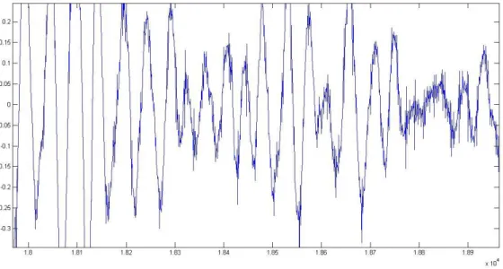
4.2.1 Input
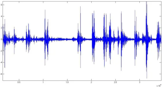
In our thesis, we have used 50,000 values in induction motor 1D signal. More values will provide more accurate signal profiling. The reason why limited values are taken is that limited values will provide much faster result in MATLAB where more than 50,000 values will create a lag while applying multiple methods. All the values are used to plot the signal file which is shown in Fig 4.2.1
18
Figure 3: 1D Input Signal of Induction Motor
4.2.2 De-noising
De-noising section provides de-noised signal from different algorithms. Each algorithm generates de-noised signal according to its implementation in MATLAB or helping algorithm which is created by ourselves. De-noised signal is slightly better signal which is then compared with original 1D signal.
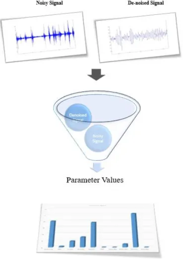
19 4.2.3 Performance Analysis
Noisy signal and de-noised signal are passed as parameters in performance analysis section.
Figure 5: Performance Analysis Technique
The idea here is to compare the signals using multiple performance analysis parameters which are already mentioned. A complete form of output data is produced from this section which are used to plot the chats such as bar chart and pie chart to picturize the comparison.
20
CHAPTER V
EXPERIMENTAL RESULT ANALYSIS
In de-noising part of our approach we have generated following signals after applying the different algorithms such as butter worth, high pass, low pass, band stop, median filter, Hilbert filter, EMD and DWT Algorithm. Each generated signal coupled with input signal is passed to performance analysis part where the signals are analyzed to gather the performance parameters.
5.1 Implementation
We are using MATLAB for this thesis which is a high-performance language for technical computing. It integrates computation, visualization, and programming in an easy-to-use environment where problems and solutions are expressed in familiar mathematical notation. We have used following features of MATLAB to implement our experimental architecture:
Math and computation Algorithm development Modeling and simulation
Data analysis, exploration, and visualization
MATLAB features a brunch of application-specific solutions called toolboxes which is directly used in this thesis. Toolbox is very important aspect asit allows to learn and apply specialized technology without learning the language of computing itself. Toolboxes are comprehensive collections of MATLAB functions (M-files) that extend the MATLAB environment to solve particular classes of problems. Here, we have used wavelet, Simulink, and basic algorithm. Areas in which toolboxes are available include signal processing, control systems, neural networks, fuzzy logic, wavelets, simulation, and many others.
We have used dwt(), butter(), hilbert(), medfilt1(),qfunc() directly to produce output signals in MATLAB.
5.2 Output Signal Analysis
Output or de-noised signals are generated by using the functional support of MATLAB or our algorithms which are described below:
21 5.2.1 Butter Worth
We have generated the output of butter worth signal using the MATLAB function butter() where the arguments are 2,0.01
Figure 6: Generated Signal of Butter Worth
The closer look of generated signal helps to understand the output of Butter worth precisely.
22 5.2.2 Low Pass Filter
We have created the output of low pass filter signal using the MATLAB function butter() where the arguments are 6,0.6
Figure 8:Generated Signal of Low Pass Filter
The closer look of generated signal helps to understand the output of Low Pass Filterprecisely.
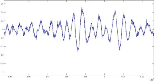
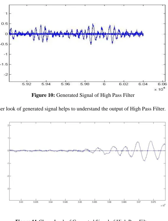
23 5.2.3 High Pass Filter
We have generated the output of high pass filter signal using the MATLAB function butter() where the arguments are 9,300/500 and 'high'
Figure 10: Generated Signal of High Pass Filter
The closer look of generated signal helps to understand the output of High Pass Filter.
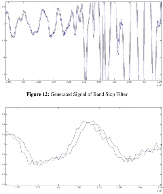
24 5.2.4 Band Stop Filter
Output of band stop filter signal is produced using same MATLAB function butter() where the arguments are 3, [0.2 0.6] and 'stop'. The closer look of generated signal helps to understand the output of Band Stop Filter.
Figure 12: Generated Signal of Band Stop Filter
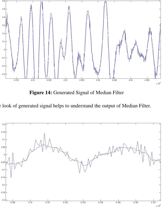
25 5.2.5 Median Filter
We have generated the output of Median filter signal using the MATLAB function medfilt1 () where the argument is only the original signal file.
Figure 14: Generated Signal of Median Filter
The closer look of generated signal helps to understand the output of Median Filter.
26 5.2.6 Hilbert Filter
We have plotted the output of Hilbert filter signal using the MATLAB function hilbert() where the argument is only the original signal file. The closer look of generated signal helps to understand the output of Hilbert Filter.
Figure 16: Generated Signal of Hilbert Filter
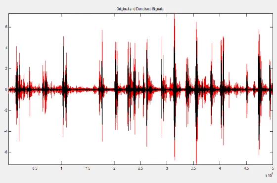
27 5.2.7 Discrete Wavelet Transform (DWT)
We have generated the output of DWT signal using the MATLAB function dwt() where the arguments are original signal file and wname. We have used db5 as a wave name value.
Figure 18: Generated Signal of DWT Algorithm and Original Signal (Red)
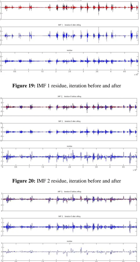
5.2.8 Empirical Mode Decomposition (EMD)
An IMF is generally formatted as a function that will follow the certain requirements:
The number of extrema and the number of zero-crossings must be equal or differ at most by one in signal data set.
The mean value of the envelope defined by the local maxima and the envelope defined by the local minima is zero at certain point or any point.
It provides a simple oscillatory aspect as a counterpart to the simple harmonic function. We can also say that IMF is any function with the same number of extrema and zero crossings, whose envelopes are symmetric with respect to zero. The IMFs of EMD records are given below:
28
Figure 19: IMF 1 residue, iteration before and after
Figure 20: IMF 2 residue, iteration before and after
29
Figure 22: IMF 4 residue, iteration before and after
Figure 23: IMF 5 residue, iteration before and after
30
Figure 25: IMF 7 residue, iteration before and after
We have reconstructed EMD output signal using 7 IMF values and two options such as OPTIONS.FIX=1 and OPTIONS.DISPLAY=1.
31 5.2.9 Gabor Filter
We have constructed the output of Gabor filter signal using the gabor filter algorithm where the arguments the original signal file,1 and 2. The closer look of generated signal helps to understand the output of GaborFilter.
Figure 27: Generated Signal of Gabor Filter
32 5.2.10 Q Function
We have constructed the output of Q function signal using the MATLAB function qfunc() where the argument is only the original signal file. The closer look of generated signal helps to understand the output of Q Function.
Figure 29: Generated Signal of Q Function
33 5.3 Parameter Value Analysis
We have gathered all the parameters value at the beginning of performance analysis section. Parameters values are serialized in excel file to draw the charts.
Table 01: Parameter Values of MSE, RMSE, MAE, SNR
Algorithm Name Mean Squared Error Root Mean Square Mean Absolute Error Signal to Noise Ratio Butter worth 0.636666 0.797914 0.388469 -24.189628 EMD 0.000639 0.025274 0.019718 30.149778 Low Pass 0.033008 0.18168 0.094287 12.401234 Band Stop 0.09186 0.303084 0.148084 7.94491 High Pass 0.574961 0.758262 0.369954 -28.73928 DWT 0.010011 0.000010 0.020001 24.803172 Hilbert Filter -0.574514 0 0.373746 -42.801259 Median Filter 0.008853 0.094091 0.050515 17.777565 Q Function 1.094552 1.046209 0.737847 -5.905687 Gabor Filter X X X -13.479976
Table 02: Parameter Values of PSNR, CC-Value, SSIM, DSSIM
Algorithm Name Peak Signal to Noise Ratio Cross Correlation Structural
Similarity Structural Dissimilarity
Butter worth -7.51671 -0.805272 0.53036 0.23482 EMD 49.26126 0.999612 1.325381 -0.162691 Low Pass 32.061924 0.971254 1.422494 -0.211247 Band Stop 27.207243 0.919899 1.424577 -0.212288 High Pass -6.195117 0.008383 0.602717 0.198642 DWT 26.493839 1 1.421403 -0.210701 Hilbert Filter 20.465832 0.707107 0.766861 0.11657 Median Filter 35.993097 0.992771 1.483348 -0.241674 Q Function -0.392366 -0.903992 0.1711 0.41445 Gabor Filter X 1 X X
34 5.4 Parameter Value Comparison
We have compared following parameters to evaluate the processing of different methods in de-noising section:
5.4.1 Mean Squared Error
According to the parameters from different methods, we have seen that Q function provides highest MSE, Hilbert Filter provides lowest MSE. EMD, DWT, Median Filter and Gabor Filter provides average MSE.
Figure 31: Mean Squared Error comparison in different parameters
35 5.4.2 Root Mean Square Error
We have noticed that Q function provides highest RMSE and DWT provides lowest RMSE. Hilbert filter, DWT, EMD and Gabor Filter generates averageRMSE.
Figure 33: Root Mean Square Error comparison in different parameters
36 5.4.3: Mean Absolute Error
According to the parameters from different methods, we have seen that Q function provides highest MAE and Gabor Filter provides lowest MAE. Here, Butter Worth, High Pass Filter and Hilbert Filter provides average MSE.
Figure 35: Mean Absolute Error comparison in different parameters
37
5.4.4 Signal to Noise Ratio
It can be noticed that EMD provides highest SNR and Hilbert Filtercreates lowest SNR. Here, Low Pass Filter, Band Stop Filter and Median Filter generates average SNR.
Figure 37: Signal to Noise Ratio comparison in different parameters
38 5.4.5 Peak Signal to Noise Ratio
According to the parameters from different methods, we have seen that EMD provides highest PSNR and Gabor Filter provides lowest PSNR. Here, Low Pass Filter, Band Stop Filter, DWT and Hilbert Filter provides average PSNR.
Figure 39: Peak Signal to Noise Ratio comparison in different parameters
39 5.4.6 Cross Correlation
We have seen that DWT provides highest CC and Q function provides lowest CC. Here, EMD, DWT, Median Filter and Gabor Filter provides average CC.
Figure 41: Cross Correlation comparison in different parameters
40 5.4.7 Structural Similarity
According to the parameters from different methods, we have noticed that Median Filter provides highest SSIM and Gabor Filter provides lowest value. Here, Low Pass Filter and Band Stop Filter and DWT provides average SSIM.
Figure 43: Structural Similarity comparison in different parameters
41 5.4.8 Structural Dissimilarity
It can be seen that Q function provides highest DSSIM and Median Filter provides lowest value. Here, Low Pass Filter, Band Stop Filter and DWT provides average DSSIM.
Figure 45: Structural Dissimilarity comparison in different parameters
42
CHAPTER VI
CONCLUSIONS AND FUTURE WORKS
6.1 Concluding RemarksIn this thesis, an experimental architecture for performace analysis of 1D signal of induction motors is proposed. The original signal is passing thorough the different methods of signal processing to generate the output of de-noised signal.
We have noticed that the research methods are proving different set of parameters value for 1D signal. For generating de-noised signal, the MATLAB toolbox‟s methods are utilized for construction and reconstruction. Furthermore, to cope with multiple parameters, excel based output generation is used which is very helpful for pictorial analysis.
Finally, the performance parameters of the experimental architecture are depicted that EMD holds highest value of two parameters and Q function holds highest value of three parameters. On the other hand, DWT, Median Filter, Band Stop filter possess maximum average values of parameters. The experimental result demonstrates that the different methods are responsible for generating different parameter values which can be used to take the decision for choosing noise reduction approach.
6.2 Future Works
The potential future directions for research based on the results presented in this thesis can be characterized into the following sections.
In the real industrial environment, several kinds of faults can be occurred at a time. therefore, the monitoring techniques should be improved to support multiple combined faults. In future we will apply Acoustic Emission Sensor (AC), Wavelet Neural Network, Terrestrial Laser Scanning (TLS), Susan filter etc.
In future we will use new parameter which is time frequency feature parameter and can meaningfully lessen performance degradation in the dissimilarity between several kinds of faults which can be occurred in the induction motor.
Different statistical classifiers, including both controlled and uncontrolled should be examined with the target of producing a reliable fault diagnosing system for induction motors.
43
REFERENCES
[1] Khan MT, Arora D, Shukla S. Feature extraction through iris images using 1-D Gabor filter on different iris datasets. Sixth International Conference on Contemporary Computing (IC3) 2013; 445-450.
[2] Sin ML, Soong WL, Ertugrul N. Induction machine on-line condition monitoring and faults diagnosis – a survey. AUPEC 2003; 1-6.
[3] W.T. Thomson and R.J. Gilmore, “Motor current signature analysis to detect faults in induction motor derives-Fundamentals, data interpretation, and industrial case histories‟, proceedings of 32nd Turbomachinery symposium, Texas, A&M university, USA, 2003. [4] IAS Motor Reliability Working Group, “Report of large motor reliability survey of industrial and commercial installation, part I,” IEEE Transactions on Industry Applications, vol. IA-21, pp. 853-864, July/Aug., 1985.
[5] J. Sottile and J. L. Kohler, “An on-line method to detect incipient failure of turn insulation in random-wound motors,” IEEE Transactions on Energy Conversion, vol. 8, no. 4, pp. 762-768, December, 1993.
[6] S. B. Lee, R. M. Tallam, and T. G. Habetler, “A robust, on-line turn-fault detection technique for induction machines based on monitoring the sequence component impedance matrix,” IEEE Transactions on Power Electronics, Vol. 18, No. 3, pp. 865-872, May, 2003. [7] A. H. Bonnet and G. C. Soukup, “Cause and analysis of stator and rotor failures in threephasesquirrel case induction motors,” IEEE Transactions Industry Application, Vol., 28, No.4, pp. 921-937, July/August, 1992.
[8] Dorrell, D. G., Thomson W. T., and Roach, S., “Analysis of air-gap flux, current, and vibration signals as function of a combination of static and dynamic eccentricity in 3-166 phase induction motors”, IEEE Transactions on Industry Applications, Vol. 33, Jan./Feb., pp. 24-34, 1997.
[9] Wu, S., and Chow, T. W. S. “Induction machine fault detection using SOM-based RBF neural networks”, IEEE Transactions on Industrial Electronics, Vol. 51, No. 1, February, pp. 183-194, 2004.
[10] S. Nandi and H. A. Toliyat, “Condition monitoring and fault diagnosis of electrical machines – a review,” in Proc. 34th Annual Meeting of the IEEE Industry Applications, pp. 197-204, 1999.
44
[11] Grassberger, P., T. Schreiber, and C. Schaffrath, „„Non-Linear Time Sequence Analysis,‟‟ Int. J. Bifurcation Chaos, 1, 521 1991 .
[12] Islam. R, Uddin. Jia, kim.J.M, “Reliable Fault Diagnosis of Induction Motors using an Acoustic Emission Sensor and Signal Processing Techniques,” The 2nd FTRA International Conference on Ubiquitous Computing Application and Wireless Sensor Network (UCAWSN-14)
[13] Xing1.W, Qi.X, and Baojin2.Li, “Rolling Bearing Fault Diagnosis based on Time-frequency Feature Parameters and Wavelet Neural Network,” International Journal of Control and Automation Vol. 8, No. 4 (2015), pp. 45-52 http://dx.doi.org/10.14257/ijca.2015.8.4.6 [14] S. Gaci, "The Use of Wavelet-Based Denoising Techniques to Enhance the First-Arrival Picking on Seismic Traces," IEEE Trans. on Geoscience and Remote Sensing, vol. 52, no. 8, pp. 4558-4563, 2014.
[15] A. C. To, J. R. Moore, and S. D. Glaser, "Wavelet denoising techniques with applications to experimental geophysical data," Elsevier Signal Processing, vol. 89, no. 2, pp. 144-160, 2009.
[16] S. Sriram, S. Nitin, K. M. M. Prabhu, and M. J. Bastiaans, "Signal denoising techniques for partial discharge measurements," IEEE Trans. on Dielectrics and Electrical Insulation, vol. 12, no. 6, pp. 1182-1191, 2005.
[17]Birgé, L., Pascal, M., 1997. From Model Selection to Adaptive Estimation.In Festschrift for Lucien Le Cam. Pollard, D., Torgersen, E., Yang, G. L. (eds.), pp. 55–87. Springer New York.
[18] Chai1, and R. R.Draxler, Root mean square error (RMSE) or mean absolute error (MAE)? –Arguments against avoiding RMSE in the literature,Air Resources University of Maryland, College Park, USA
[19]Donoho, D. L., Johnstone, J. M., 1994. Ideal Spatial Adaptation by Wavelet Shrinkage.Biometrika, vol. 81 (3), pp. 425–55.
[20] Andreas Antoniou (2006) Digital Signal Processing. McGraw Hill, USA.
[21] Alan V. Oppenheim, Ronald W. Schafer (1989) Discrete-Time Signal Processing. Prentice Hall, USA.
[22] R. L. C. Van Spaendonck, F. C. A. Fernandez, R. G. Baraniuk and J.T. Fokkema (2002),Local Hilbert transformation for seismic attributes. EAGE 64th Conference and Technical Exhibition.
[23] Jose G. R. C. Gomes and A. Petraglia (2002), An analog Sampled-data DSB to SSB converter using recursive Hilbert transformer for accurate I and Q channel matching.
45 IEEE Trans. Circ. Syst. II, vol. 49, no. 3, pp. 177-187.
[24] Michael Feldman (2011), Hilbert transform in vibration analysis. Mechanical Systemsand Signal Processing, no. 25, pp. 735-802.
[25] Khan MT, Arora D, Shukla S., Feature extraction through iris images using 1-D Gabor filter on different iris datasets. Sixth International Conference on Contemporary Computing (IC3) 2013.