Buffer Management Method for Multiple
Projects in the CCPM-MPL Representation
Nguyen Thi Ngoc Truc*
Department of Information Science and Control Engineering, Nagaoka University of Technology, Nagaoka, Japan Yoshinori Takei
Department of Electrical Engineering, Nagaoka University of Technology, Nagaoka, Japan Hiroyuki Goto
Department of Industrial and Systems Engineering, Hosei University, Koganei, Japan Hirotaka Takahashi
Department of Humanities, Yamanashi Eiwa College, Kofu, Japan
(Received: August 19, 2012 / Revised: November 23, 2012 / Accepted: November 26, 2012) ABSTRACT
This research proposes a framework of buffer management for multi-project systems in the critical chain project man-agement (CCPM) method, expressed in the form of max-plus linear (MPL) representation. Since time buffers are in-serted in the projects for absorbing uncertainties in task durations and protecting the completion times, the proposed method provides a procedure for frequently surveying the rates of consumed buffers and the rate of elapsed times. Their relation expresses the performance of the projects which is plotted on a chart through the completed processes. The chart presents the current performance of the projects and their interaction, which alerts managers to make neces-sary decisions at the right time for managing each project and the entire multi-project system. The proposed frame-work can analyze the complex system readily, and it enables managers to make an effective decision on scheduling. The effectiveness of the framework is demonstrated through a numerical example.
Keywords: Max-Plus Linear System, Critical Chain Project Management, Time Buffers, Multiple Projects, Buffer Management, Fever Chart
* Corresponding Author, E-mail: [email protected]
1. INTRODUCTION
The critical chain project management (CCPM) is a well-known method for planning and managing projects. The concept of the CCPM is an outgrowth of the theory of constrains (TOC), first developed by Goldratt (1990), which has drawn much attention for many researchers (Herroelen et al., 2002; Cohen et al., 2004; Leach, 2005; Tukel et al., 2006). These researches have mainly fo-cused on clarifying the concepts of the CCPM method, discussing several related issues such as resource con-flict, buffer’s size, and buffer management. In project
management, initial schedule is frequently changed due to unpredictable reasons such as external uncertainties, processing changes, and resource conflicts. Thus, the CCPM provides a method for inserting time buffers which play a role for absorbing uncertainties in the task durations to protect the completion time. Moreover, the CCPM method has achieved successes not only for a single project but for large-scale multi-projects (Cohen
et al., 2004; Leach, 2005).
On the other hand, the max-plus linear (MPL) rep-resentation is known as an efficient tool for describing a class of discrete event systems (DESs) (Heidergott et al., Vol 11, No 4, December 2012, pp.397-405 http://dx.doi.org/10.7232/iems.2012.11.4.397
2006; Goto, 2010). The typical and significant feature of DESs is that events occur at discrete time instants and the values of the internal states change non-continuously. This kind of systems typically appears in manufacturing systems, transportation systems, project management, and so on. Since unpredictable changes in the execution times may influence the completion time, several re-searches that consider uncertainties have been carried out (Heidergott, 2006). However, due to the nonlinearity in the states of the system, it is difficult to handle large-scale systems.
Furthermore, an application of the CCPM frame-work to an MPL representation was studied in our pre-vious paper (Takahashi et al., 2009; Truc et al., 2011). Therein, a method for determining and inserting time buffers to absorb uncertainties is considered using an MPL representation. We first identified a critical path, which is the longest path of successive tasks with zero float time. Then, we reduced the processing time and installed project and feeding buffers. A project buffer is inserted between the end of the critical path and its suc-ceeding output. Feeding buffers are inserted wherever a non-critical path joins into a critical path. These buffers were frequently monitored and controlled with a buffer management policy (Kasahara et al., 2009), in which the behavior of a project is featured by the rates of buffer consumption and processing time. However, these works were designed only for a single-project system.
Recently, a CCPM-MPL framework for determin-ing time buffers has been proposed for multi-project systems (Truc et al., 2012), an extended and improved version of a single-project case. The project and feeding buffers are determined for each project in large-scale systems; the buffers are used to absorb uncertainties in the internal task durations of each project. Moreover, the constraints between the projects are determined to insert capacity buffers; they play a role for absorbing uncer-tainties in the preceding project and protect the subse-quent projects.
This research considers a framework for managing these buffers in a multi-project system. Particularly, instead of minimizing the duration of each project as the case of a single project, the multi-project scheduling aims to maximize the throughput of the entire system by sharing the same resources. Thus, it is difficult for man-agers to comprehend the relationship between these pro-jects with mutual dependence by applying the single-project framework (Kasahara et al., 2009) one by one, making the control of the whole system tough. The pro-posed framework herein expresses the performance for all projects and their relationship in the complex system with multiple input times, which can alert managers to make extra actions at the proper time to avoid tardiness both for individual project and for the entire system. In this paper, the effect of cost and resource conflicts is not considered for the sake of simplicity. For further discus-sion of resource conflicts, refer to Yoshida et al. (2011).
The remaining contents are presented in the
follow-ing four sections. Section 2 provides a brief review of the theoretical background for this paper: max-plus al-gebra, MPL representation, and CCPM-MPL framework. Section 3 derives a concept of buffer management in the CCPM method, and proposes a framework of buffer management in the form of the MPL representation. The proposed framework is confirmed through a numerical example in Section 4. Finally, conclusions and recom-mendations are given in Section 5.
2. THEORETICAL BACKGROUND 2.1 Max-Plus Algebra
Max-plus algebra is known as the schedule algebra for describing a certain class of DESs. For a set D=R
{−∞}, where R is the entire real set, operators for addi-tion and multiplicaaddi-tion are defined as:
max( , ),
⊕ = ⊗ = +
x y x y x y x y (1)
The symbol ⊗ corresponds to multiplication in conventional algebra, and is often omitted when no con-fusion is likely to arise. For example, we simply write xy
for expressing x⊗y. These operators hold the commu-tative, associative and distributive laws. The zero and unit elements for these are given by ε(= −∞) and e
( 0),= respectively. These hold x⊕ = ⊕ =ε ε x ε and x
ε ε ε
⊗ = ⊗ =x for an arbitrary ε(= +∞).Moreover, we define ε(= +∞) and assume a property ε ε⊗ = ⊗ =ε ε ε.
Furthermore, the following two operators are de-fined for subsequent discussions:
min( , ),
∧ = : =− +
x y x y x y x y (2)
An operator for the power of a R∈ is defined as:
.
⊗a= ×
x x a (3) Operators for multiple numbers are as follows. If m≤n,
1 max( , , , ), = + ⊕n = " k m kx x xm m xn (4) 1 min( , , , ). = + ∧n = " k m kx x xm m xn (5) For a matrix X∈Dm n× , [ ] j i
X expresses the (i, j)th ele-ment of X, and XT is the transpose matrix of X. For
, ∈Dm n×,
X Y
[X⊕Y]ij=max
(
[ ] [ ]X ij, Y ij)
(6)[X Y∧ ]ij=min
(
[ ] [ ]X ij, Y ij)
(7) If X∈Dm l×,Y∈Dl p× ,[X⊕Y]ij= ⊕lk=1
(
[ ] [ ]X ij, Y ij)
(8)[X:Y]ij= ∧lk=1
(
[ ] [ ]X ij, Y ij)
(9) The priority of operators ⊗ and : are higher than that of operators ⊕ and ∧ where : is well-defined if X has at least one non-ε entry in every row. The zero and unit elements for matrices are; εmn is a matrixwhose all elements are ε in Dm n× , and e is a matrix
whose diagonal elements are e and off-diagonal ele-ments are ε. For a vector v∈Dm, diag( )v ∈Dm n×
repre-sents a matrix whose diagonal elements are [ ]vi and off-diagonal elements are ε.
2.2 Max-Plus Linear Representation
We briefly review the MPL representation for a certain class of discrete event systems developed by Yoshida et al. (2010). We assume the following con-straints imposed on the focused system:
• The number of processes, external inputs and external outputs are n, p, and q, respectively.
• All processes are used only once for a single job. • The subsequent job cannot start processing while the
current job is at work.
• Processes that have precedence constraints cannot start processing until they have received all the re-quired parts from the preceding processes.
• Processes with external inputs cannot start until all the required materials have arrived.
• The processing starts as soon as all the conditions above are satisfied.
For the kth job in process i(1≤ ≤i n), let ( )( 0),≥
i d k ( ) , − ⎡ ⎤ ⎢ ⎥ ⎣x k ⎦i and ( ) , + ⎡ ⎤ ⎢ ⎥
⎣x k ⎦i be the processing time,
process-ing start time, and processprocess-ing completion time, respec-tively. We give the initial condition by x(0)=εn1. More-over, [u( )k ]i represents the material arrival time from external input i(1≤ ≤i p), and [y( )k ]i represents the output time of the finished product to external output
(1≤ ≤ ).
i i q The following matrices P F Bk, 0, 0 and C0 are introduced for representing the structure of the sys-tem:
[ ]Pkij={d ki( ) : ifi= j, : otherwiseε }
[ ]0
: if process has a preceding process ,
: if process does not have a preceding process ,
ε ⎧⎪⎪ = ⎨ ⎪⎪⎩ ij e i j i j F [ ]0
: if process has an exterrnal input , : if process does not have an external input ,
ε ⎧⎪⎪ = ⎨ ⎪⎪⎩ ij e i j i j B [ ]0
: if process has an exterrnal output , : if process does not have an external output ,
ε ⎧⎪⎪ = ⎨ ⎪⎪⎩ ij e i j i j C
where F B0, 0 and C0 are referred to as the adjacency, input and output matrices, respectively.
The earliest completion time is defined as the
mini-mum value with which the corresponding process can complete processing. Specifically, the earliest comple-tion times of all processes are calculated by:
* 0 0 ( ) ( ) [ ( 1) ( )], + = + + − ⊕ E k k x k P F P x k B uk (10) where * 1 0 0 0 ( ) ⊕ ⊕"⊕( ) ,l− k n k k P F e P F P F and an instance (1≤ ≤ )
l l n depends on the precedence-relationships of the system. The corresponding output times are given by:
0
( )= ⊗ +( )
E k E k
y C x (11)
The earliest starting times of all processes are given by:
( ) ( ).
− = : +
E k k E k
x P x (12)
Furthermore, the latest starting times are defined as the maximum value by which the same output time based on the earliest time can be accomplished. Thus, the latest starting times of all processes and the latest feeding times are given by:
* 0 0 ( ) ( ) ( ) − ⎡ ⎤ ⎡ ⎤ = ⎢⎣ ⎥⎦ :⎢⎣ T: ⎥⎦ L k k k T C E k x P F P y (13) 0 ( )= T: −( ) L k L k u B x (14)
A critical path is understood as a series of proc-esses with zero total float. Total float is the maximum time which can be moved backward without changing the completion time. This is defined as the difference between the latest and earliest starting times. Specifi-cally, the total floats ω( )k of all processes are obtained as:
(
)
( )=diag −( ) : −( ) E L k x k x k ω (15)Moreover, the critical path is identified by the set of process numbers α that satisfy:
[ ]
{
α ω( )k α=0}
(16)2.3 CCPM-MPL Framework for Determining Time Buffers in Multiple Projects
We briefly review the framework for determining time buffers in a multi-project system (Truc et al., 2012). Considering a general system with m processes (tasks) and n projects, n vectors 1 2l l, ,",lnof m-dimension are
introduced with the following properties:
: if process belongs to project , : otherwise ε ⎧⎪⎪ ⎡ ⎤ = ⎨ ⎢ ⎥ ⎣ ⎦j i ⎪⎪⎩ e i j l (17)
for all i(1≤ ≤i m) and j(1≤ ≤j n), and lj expresses
which processes belong to project j. Note that process i
on the priority of the projects and the processes. Then, we define a matrix L∈Dm n× that represents the layer of
projects as follows:
[ 1 2 ] = " n
L l l l (18)
Moreover, we reduce the processing time of tasks to 1/3 of the original time and define the size of time buffers as 1/3 of the corresponding path duration (Taka-hashi et al., 2009). The position and size of the buffers are determined as below:
• Project buffer (PB)
Project buffers are inserted between the end of critical paths and their succeeding external outputs, to protect the critical paths. The positions are determined by inspecting the elements of the output matrix C0, if [ ]C0ij≠ε and j∈α, a PB is inserted behind process. The sizes of the PBs are obtained by:
1 3 (diag( α ) ) ⊗ − = T: : p L E b L x y (19)
where matrix Lα is defined from the set of critical proc-esses (α) determined in Eq. (16) as:
[ ] : if and ,[ ] : otherwise α α ε ⎧⎪ ∈ ⎪ = ⎨ ⎪⎪⎩ ij ij e i L = e L (20) • Feeding buffer (FB)
Feeding buffers are inserted where a non-critical path joins into a critical path, to protect the critical paths from delay which may occur in the non-critical paths. To define the positions of FBs, we first introduce two vectors v and w with the properties as[ ]vi={ :e i∈β ε, :
},
β
∉
i and[ ]wi={e i: ∈α ε, :i∉α}, where β is the set of non-critical processes, the positions are identified using two vectors v′ and w′ with the following proper-ties: : if , : otherwise, βα γ ε ⎧ ∈ ⎪⎪ ⎡ ⎤ ⎡ ⎤′ =⎢ ⊗ ⎥ = ⎨ ⎣ ⎦i ⎣ T ⎦i ⎪⎪⎩ e i v F w (21)
where γ is the subset of β having a successor classi-fied asα.Fβα=diag( )w ⊗F0⊗diag( ),v Fβα represents the transitions from non-critical processes to critical ones.
: if , : otherwise, βα τ ε ⎧ ∈ ⎪⎪ ⎡ ⎤ ⎡ ⎤′ =⎢ ⊗ ⎥ = ⎨ ⎣ ⎦i ⎣ ⎦i ⎪⎪⎩ e i w F v (22)
where τ is the subset of α having a predecessor classi-fied as β. Then, FBs are installed at transitions between processes γ and τ. The sizes of the FBs are estimated as: 1 3 * (diag( ) ( ββ ) ) ⊗ ′ = ⊗ ⊗ ⊗ ⊗ f k k b P v F P v (23)
where Fββ=diag( )v ⊗F0⊗diag( ),v Fββrepresents the tran-sitions from non-critical processes to non-critical ones.
• Capacity buffer (CB)
Capacity buffers are inserted at the transitions be-tween projects, to absorb uncertainties in the preceding project and protect the subsequent projects. We first determine transitions for each pair of the projects. Gen-erally, transitions from project A to project B(A≠B) are defined through two vectors h and h′ with the follow-ing properties as:
: if , : otherwise, βα τ ε ⎧ ∈ ⎪⎪ ⎡ ⎤ ⎡ ⎤′ =⎢ ⊗ ⎥ = ⎨ ⎣ ⎦i ⎣ ⎦i ⎪⎪⎩ e i v w F (24)
where ϑ is the set of processes in project A with a suc-cessor belonging to project B. FAB=diag ( )lB ⊗F0diag
( ),lA FAB represents the transitions from processes in
project Ato processes in project B.
[ ] : if , : otherwise, ϕ ε ⎧ ∈ ⎪⎪ ⎡ ⎤ =⎢⎣ AB⊗ A⎥⎦ = ⎨⎪⎪⎩ i i e i hw F l (25)
where ϕ is the set of processes in project B with a predecessor belonging to project A. Taking these to-gether, CBs are inserted at transitions between processes ϑ andϕ. The sizes of the CBsfrom project A to B are calculated by: 1 3 (diag( ) ( ) * )⊗ = ⊗ ⊗ ⊗ ⊗ c k AA k A b P h F P l (26)
where FAA=diag( )lA ⊗F0⊗diag( ).lA FAA represents the
transitions between processes in project A.
Similarly, we can find the positions and sizes of CBs from project B to A, or between any pair of the projects.
• Redefined system with the CCPM applied
The representing matrices introduced in Section 2.2 are redefined for easily comprehending the structure of the system after the CCPM applied. After the insertion of the PB, the output matrix Cγ is reformulated in the
following manner:
0
diag( ) ,
= p ⊗
Cγ b C (27)
where the subscript ‘γ’ expresses that the matrix was redefined. After the insertion of the FBs and CBs, the adjacency matrix Fγ is reformulated as:
0 ,
γ= ⊕ βα⊕ c
F F F F (28) where Fβα=Fβα⊗diag( ) :bf Fβα and bf expresses the
po-sition and sizes of the FBs, respectively, and
(
)
(
)
, 1 diag ( ) , = ≠ =⊕
n ⊗ c xy c xy x y x y F F b (29)where n is the number of projects. The subscript ‘c’ ex-presses the CBs. Fxy presents the transitions of
proc-esses from project x to y, and ( )bc xy expresses the size of
the corresponding CBs. Note that Fc=εmn if n = 1. Moreover, matrices = ⊗1/ 3
k
Pγ P and B0 remain unchanged.
3. BUFFER MANAGEMENT 3.1 Concept of the CCPM
In the CCPM, for managing and observing the pro-jects’ performance, the buffers are frequently monitored to protect the critical path as well as the project’s com-pletion time. This mechanism is called “Buffer Man-agement”, which can detect a potential problem and raise a warning signal to managers. As the projects proceed, if a task elapses a longer time than expected, the task con-sumes the buffer on the corresponding path. Thus, the buffer management frequently compares two parame-ters: the consumption rate of the PB and the progress rate of the corresponding critical path, for expressing the current performance of the project. In the multi-project system, these parameters are frequently checked for all projects and plotted on a fever chart, as shown in Figure 1. This chart shows the relationship between buffer used (%) versus time used (%) through the completed proc-esses. The chart is divided into three zones: green, yel-low, and red, which are determined empirically by thre-sholds settings. Typically, we base on the threthre-sholds settings proposed by Leach (2005) as listed in Table 1.
Figure 1. An example of a fever chart. Table 1. Buffer thresholds
Buffer used (%)
Time used (%) Green to yellow
transition (%)
Yellow to red transition (%)
0
100 15 75 30 90
Using the fever chart, the projects’ status is alerted to project managers and the decision level for an extra action is suggested. Specifically, if the current status is in the green zone, the project is going well and the man-agers need not take an action. If the status is in the yel-low zone, the project assesses a problem and needs a recovery plan to avoid further buffer erosion. If the status is in the red zone, the project will possibly be late and the managers should initiate the action.
3.2 Proposed Method
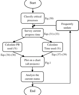
We develop a framework of buffer management for a multi-project system, which focuses on the system after the insertion of the time buffers. The overall pro-cedure for buffer management is summarized as the flowchart in Figure 2. A sequencing description for the procedure is expressed by using the MPL representation as follows: Fig.1 Eqs.(37)-(39) Eqs.(34)-(36) Eqs.(31)-(33) Eq.(30) Calculate Time used (%) Start Classify critical processes Survey current progress time Calculate PB used (%) Plot on a chart (all projects) Analyze the current status End Frequently update
Figure 2. Flowchart of buffer management. We again consider the multi-project system with n
projects and m processes mentioned in Section 2.3. Us-ing n vectors (l l1, ,2 ",ln) which represent the processes
belonging to n projects, derived in Eq. (17), we define n
vectors l1α,l2α,",lnα that satisfy:
[ ] : and [ ] , : otherwise, α α α ε ⎧⎪ ∈ = ⎪ = ⎨ ⎪⎪⎩ x i x i e if i l e l (30)
where α is the set of critical processes determined by Eq. (16), and lxα expresses which critical processes
be-long to project x(1≤ ≤x n). Thus, the managers can mo-nitor each project in only one procedure for the entire system instead of considering them independently. Next, we introduce a vector z which represents the actual completion times of the completed processes at the monitoring stage. Thus, the managers can survey the value of this vector frequently whenever monitoring the project’s execution. Vector z has the following property:
[ ] : , : otherwise, βα η ε ⎧ ∈ ⎪⎪ ⎡ ⎤ =⎢⎣ ⊗ ⎥⎦ = ⎨⎪⎪⎩i i i t i v z F (31)
where ti is defined as actual completion time of process
i and η represents the set of completed process numbers at the monitoring stage, and ε(= +∞) is mentioned in Section 2.1. In order to manage the buffers for each pro-ject, we decompose vector z to n vectors z z1, ,1 ",zn,
which represent n projects by:
diag( ) α,
= ⊗
x x
z z l (32)
where x∈{1,",n}, and z has the following properties:
[ ] : , : otherwise, βα η ε ⎧ ∈ ⎪⎪ ⎡ ⎤ =⎢⎣ ⊗ ⎥⎦ = ⎨⎪⎪⎩i i i t i v z F (33)
In order to know the projects’ performance at the monitoring stage, we calculate the rates of the PBs’ con-sumption and the elapsed times. These values are deter-mined for each project as the following procedure:
• Ratio of the PBs’ consumption (buffer used, %): First, we classify the original PB for each project (x):
0 α, = T⊗ ⊗
px p x
b b C l (34)
where bp is the size of the PBs obtained from Eq. (19).
Then, we define the PB consumed by the completed processes for project (x) using the following vector:
( ) =diag( + ): ,
x used xE x
b γ z (35)
where +
R
xγ presents the earliest completion times of the
system after the CCPM application, derived in Section 2.3. Finally, the consumption rate of the PB at the mo-nitoring stage is calculated through vector rb as:
1
( ) ⊗ .
= bpx
bx x used
r b (36)
• Ratio of the progress time over the critical path duration (time elapsed, %)
First, we calculate the duration time of the critical path for each project (x):
0 (diag( γ′ ) γ ) α = : T⊗ x L E x d u y C l (37) where γ α , γ − ′ = T : ′ L L L
u L xγ u expresses the latest feeding
times on the critical paths, and −
L
xγ and yγE are the
lat-est starting times and the output times of the system after the CCPM application, derived in Section 2.3. Then, we define the completion time of processes at the monitoring stage without considering the effect of input times as: 0 ( α γ ) . ′ = T : : x x L x z l B u z (38)
where uγL expresses the latest feeding times which is
derived in Section 2.3. Finally, the ratio of the progress time over the estimated completion time is obtained through vector rtx as:
1 . ⊗ ′ = dx tx x r z (39)
The ratio of buffer consumption (%) versus the cor-responding progress time (%) is plotted, respectively for all projects through the completed processes on the same fever chart (Figure 1). The chart expresses the current status of all projects and their interaction. Thus, managers can make a proper decision for protecting each project and the entire system.
4. NUMERICAL EXAMPLE
A numerical example for a simple system is pre-sented to facilitate better understanding of the proposed framework.
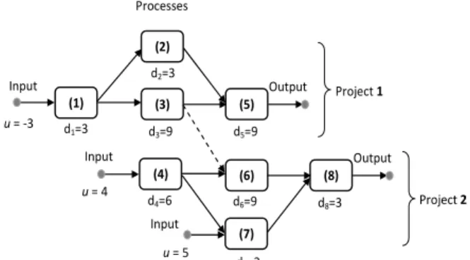
Figure 3 shows a simple system with two projects consisting of three inputs, two outputs and eight pro-cesses. Note that the dashed arrow from process (3) to (6) is considered as the precedence constraint between the two projects.
Project 1 consists of processes (1), (2), (3), and (5).
Project 2 consists of processes (4), (6), (7), and (8).
u= 5 u= 4 d7=3 u= ‐3 Project 1 Project 2 d2=3 Input Output d1=3 d3=9 d5=9 Processes (3) (1) (5) Input Output d6=9 d8=3 (6) d4=6 (4) (8) (2) (7) Input
Figure 3. A simple system with two projects (1 and 2). 4.1 Determination of Time Buffers
Using the MPL representation introduced in Sec-tion 2.2, the representaSec-tion matrices for the entire sys-tem are given as follows:
0 , ε ε ε ε ε ε ε ε ε ε ε ε ε ε ε ε ε ε ε ε ε ε ε ε ε ε ε ε ε ε ε ε ε ε ε ε ε ε ε ε ε ε ε ε ε ε ε ε ε ε ε ε ε ε ε ⎡ ⎤ ⎢ ⎥ ⎢ ⎥ ⎢ ⎥ ⎢ ⎥ ⎢ ⎥ ⎢ ⎥ ⎢ ⎥ = ⎢ ⎥ ⎢ ⎥ ⎢ ⎥ ⎢ ⎥ ⎢ ⎥ ⎢ ⎥ ⎢ ⎥ ⎢ ⎥ ⎣ ⎦ e e e e e e e e e F 0 ε ε ε ε ε ε ε, ε ε ε ε ε ε ε ⎡ ⎤ ⎢ ⎥ = ⎢⎣ ⎥⎦ e e C diag(3, 3, 9, 6, 9, 9, 3, 3) = k P 0 . ε ε ε ε ε ε ε ε ε ε ε ε ε ε ε ε ε ε ε ε ε ε ⎡ ⎤ ⎢ ⎥ ⎢ ⎥ = ⎢ ⎥ ⎢ ⎥ ⎣ ⎦ T e e B
Assuming that the initial condition is x(0)=ε81 and the input times u= −[ 3 4 5] ,T the output times and the
criti-cal path are identified as =(18 22)T E
y and α={1, 3, 4, 5, 6, 8}. respectively.
Moreover, we apply the MPL representation pre-sented in Section 2.3 to the system. First, the processing times are given by (3, 3, 9, 6, 9, 9, 3, 3)⊗1/ 3.
From Eq. (17), we define two vectors as: 1=( ε ε ε ε) ,
T
e e e e
l l2=(ε ε ε εe e e e) .T
The matrix L given in Eq. (18) is:
, ε ε ε ε ε ε ε ε ⎡ ⎤ ⎢ ⎥ = ⎢⎣ ⎥⎦ e e e e e e e e L • Project buffer
Since the critical path is identified as α={1, 3, 4, 5, 6, 8}, and[ ]C0 15=e and[ ]C0 28=e the positions of the PBs are behind processes (5) and (8). From Eqs. (19) and (20), we obtain the sizes of the PBs as =(7 6) .T
p
b • Feeding buffer
From Eqs. (21)–(23), we obtain the positions of the FBs inserted at the transitions of process (2) → (5) and process (7) → (8). The sizes of the FBs are determined
as =( 1ε ε ε ε ε ε1 ) .T f
b
• Capacity buffer
From Eqs. (24)–(26), a CB is inserted at the transi-tion of process (3) → (6). Moreover, the size of the CB at the transition from project 1 to 2 is ( )bc 12=(ε ε ε ε4
) .
ε ε εT
Figure 4 shows the system with the time buffers in-serted for the multi-project system in Figure 3.
• The system with the CCPM applied
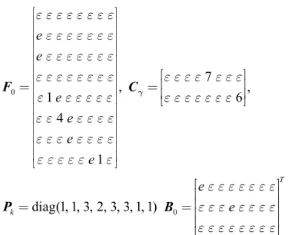
The matrices for representing the structure of the latter system are redefined as follows. Using Eqs. (27)– (29), we obtain the adjacency and output matrices as:
0 1 , 4 1 ε ε ε ε ε ε ε ε ε ε ε ε ε ε ε ε ε ε ε ε ε ε ε ε ε ε ε ε ε ε ε ε ε ε ε ε ε ε ε ε ε ε ε ε ε ε ε ε ε ε ε ε ε ε ε ⎡ ⎤ ⎢ ⎥ ⎢ ⎥ ⎢ ⎥ ⎢ ⎥ ⎢ ⎥ ⎢ ⎥ ⎢ ⎥ = ⎢ ⎥ ⎢ ⎥ ⎢ ⎥ ⎢ ⎥ ⎢ ⎥ ⎢ ⎥ ⎢ ⎥ ⎢ ⎥ ⎣ ⎦ e e e e e e F 7 , 6 ε ε ε ε ε ε ε ε ε ε ε ε ε ε ⎡ ⎤ ⎢ ⎥ = ⎢⎣ ⎥⎦ Cγ diag(1, 1, 3, 2, 3, 3, 1, 1) = k P 0 ε ε ε ε ε ε ε ε ε ε ε ε ε ε ε ε ε ε ε ε ε ε ⎡ ⎤ ⎢ ⎥ ⎢ ⎥ = ⎢ ⎥ ⎢ ⎥ ⎣ ⎦ T e e B
Using Eqs. (10)-(16), the earliest completion times and the corresponding output times are calculated as
( 2 11 6 4 9 7 10)
γ
+ = − − T
E
x and yγE=(11 16)
respecti-vely. The latest feeding times are obtained as uγL=
( 3 4 7)− T. Moreover, the critical path is identified as {1, 3, 4, 5, 6, 8}
α= .
4.2 Buffer Management
After the insertion of the time buffers, the multi-project system is monitored and controlled through the
Output Output d2=1 FB=1 CB=4 u= 5 u = ‐3 Input d1=1 d3=3 d5=3 Processes (3) (1) (5) Input Input d4=2 d6=3 d8=1 (6) (4) (8) u= 4 CB FB=1 d7=1 (7) FB (2) FB PB=7 PB PB=6 PB Project 1 Project 2
buffer management proposed in Section 3.2. From Eq. (30), we obtain two vectors as:
[ ] 1α= ε ε ε ε ε , T e e e l [ ] 2α=ε ε ε ε ε . T e e e l
We assume here that the set of the completed pro-cesses η and the vector of the actual completion times z have been collected at the motoring stage as:
{1, 2, 3, 4, 6, 7}
η=
(0 2 6 7 11 8 )ε ε
= T
z
Using Eq. (32), we decompose z into:
[ ] 1=diag( )⊗1α=0 6ε ε ε ε ε ε T z z l [ ] 2=diag( )⊗ 2α=ε ε ε ε7 11ε ε T z z l
• Ratio of the PB’s consumption
- Classify the original PB of each project: 1= T⊗ 0⊗1α=7 p p b b C l 2= T⊗ 0⊗ 2α=6 p p b b C l
- Define the PBs consumed by the completed pro-cesses on each project (buffer used):
1 1 ( ) =diag( + ): used xE b γ z [2 5ε ε ε ε ε ε] , = T 2 2 ( ) =diag( +): used xE b γ z [ε ε ε ε ε ε1 2 ] , = T
• Ratio of the corresponding progress time over the expected duration time
- Calculate the duration time of the critical path for each project: 3 . 4 α γ− ⎡− ⎤ ⎢ ⎥ ′ = = ⎢ ⎥ ⎣ ⎦ : T rL L u L x 1=(diag( γ′L): rE)T⊗ 0 1α=14 d u y C l 2=(diag( γ′L): rE)T⊗ 0 2α=12 d u y C l
- Define the progress time at the monitoring stage without considering the effect of the input time (time used): [ ] 1′ =(1α: 0 γ ): 1=3 9ε ε ε ε ε , T T L z l B u z [ ] 2′ =(2α: 0 γ ): 2=ε ε ε ε ε ε3 7 , T T L z l B u z
- Obtain the ratio of the progress time over the dura-tion time of the critical path (time used, %):
1 1 1 1 3 9 , 14 ε 14 ε ε ε ε ε ⊗ ⎡ ⎤ ′ ⎢ ⎥ = = ⎢ ⎥ ⎣ ⎦ d T t z r 1 2 1 2 3 7 . 12 12 ε ε ε ε ε ε ⊗ ⎡ ⎤ ′ ⎢ ⎥ = = ⎢ ⎥ ⎣ ⎦ d T t z r
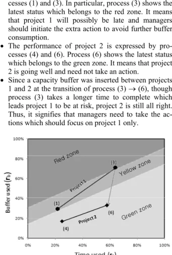
The ratio of buffer consumption versus the corre-sponding progress time is plotted on a fever chart as shown in Figure 5. The plotted points express the sta-tuses of the completed processes along the critical paths. The chart implies the following:
• The performance of project 1 is expressed by pro-cesses (1) and (3). In particular, process (3) shows the latest status which belongs to the red zone. It means that project 1 will possibly be late and managers should initiate the extra action to avoid further buffer consumption.
• The performance of project 2 is expressed by pro-cesses (4) and (6). Process (6) shows the latest status which belongs to the green zone. It means that project 2 is going well and need not take an action.
• Since a capacity buffer was inserted between projects 1 and 2 at the transition of process (3) → (6), though process (3) takes a longer time to complete which leads project 1 to be at risk, project 2 is still all right. Thus, it signifies that managers need to take the ac-tions which should focus on project 1 only.
Red z one Yellow zone Green zone
Figure 5. Fever chart for the multi-project system in Figure 4.
5. CONCLUSION
We have proposed an MPL representation for de-scribing a buffer management in the CCPM method focusing on multi-project systems. By introducing an inspected vector which represents the actual completion time of the completed processes at the monitoring stage, the managers can survey the performance of all projects frequently. Moreover, the proposed method can analyze the complex system to estimate the rates of the con-sumed project buffers and the elapsed progress times readily for expressing the current status of all projects and their interaction, which support managers to easily monitor each project, effectively managing the entire system.
Since we have developed a deterministic model for inserting and controlling the time buffers, for practical cases, a stochastic model, which takes into account the
analysis of the external uncertainties, will be an impor-tant future work.
ACKNOWLEDGMENTS
Yoshinori Takei has been supported in part by a re-search grant from JSPS Grants-in-Aid for Scientific Re-search No. 23650005. Hiroyuki Goto has been suppor-ted in part by a research grant from JSPS Grants-in-Aid for Scientific Research No. 23510163. Hirotaka Takaha-shi has used the facilities of Earthquake Research Insti-tute (ERI), The University of Tokyo. He has also been supported in part by the JSPS Grant-in-Aid for Scien-tific Research No. 23740207.
REFERENCES
Cohen, I., Mandelbaum, A., and Shtub, A. (2004), Multi-project Scheduling and Control: A process-based comparative study of the Critical Chain Methodo-logy and Some Alternatives, Project Management
Journal, 35(2), 39-50.
Goldratt, E. M. (1990), Theory of Constraints, North Ri-ver Corp., Great Barington, MA.
Goto, H. (2010), Modelling methods based on discrete algebraic systems. In: Goti, A. (ed.), Discrete Event
Simulations, Sciyo, Rijeka, Croatia, 35-62.
Heidergott, B. (2006), Max-Plus Linear Stochastic
Sys-tems and Perturbation Analysis, Springer, New
York, NY.
Heidergott, B., Jan Olsder, G., and van der Woude, J. W. (2006), Max Plus at Work: Modeling and Analysis
of Synchronized Systems, Princeton University Press,
Princeton, NJ.
Herroelen, W., Leus, R., and Demeulemeester, E. (2002), Critical chain project scheduling: do not
oversim-plify, Project Management Journal, 33, 46-60. Kasahara, M., Takahashi, H., and Goto, H. (2009), On a
buffer management policy for CCPM-MPL repre-sentation, International Journal of Computational
Science, 3(6), 593-606.
Leach, L. P. (2005), Critical Chain Project Management, Artech House, Boston, MA.
Takahashi, H., Goto, H., and Kasahara, M. (2009), To-ward the application of a critical-chain-project-management-based framework on max-plus linear systems, Industrial Engineering and Management
Systems, 8(3), 155-161.
Truc, N. T. N., Goto, H., Takahashi, H., and Yoshida, S. (2011), Enhanced framework for determining time buffers in the MPL-CCPM representation, Interna-tional Journal of Information Science and
Com-puter Mathematics, 4(1), 1-18.
Truc, N. T. N., Goto, H., Takahashi, H., Yoshida, S., and Takei, Y. (2012), Critical chain project man-agement based on a max-plus linear representation for determining time buffers in multiple projects,
Journal of Advanced Mechanical Design, Systems,
and Manufacturing, 6(5), 715-727.
Tukel, O. I., Rom, W. O., and Eksioglu, S. D. (2006), An investigation of buffer sizing techniques in critical chain scheduling, European Journal of
Op-erational Research, 172(2), 401-416.
Yoshida, S., Takahashi, H., and Goto, H. (2010), Modi-fied max-plus linear representation for inserting time buffers, Proceedings of the IEEE Internatio-nal Conference on Industrial Engineering and
En-gineering Management, Macau, China, 1631-1635.
Yoshida, S., Takahashi, H., and Goto, H. (2011), Reso-lution of time and worker conflicts for a single pro-ject in a max-plus linear representation, Industrial
Engineering and Management Systems, 10(4),