Partially linear single-index beta regression model and score test

Contents lists available atScienceDirect

Journal of Multivariate Analysis

journal homepage:www.elsevier.com/locate/jmva

Partially linear single-index beta regression model and score test

✩

Zhao Weihua

a,c

, Zhang Riquan

a,b,∗

, Huang Zhensheng

d

, Feng Jingyan

b

a_{Department of Statistics, East China Normal University, Shanghai, 200062, PR China} b_{Department of Mathematics, Shanxi Datong University, Datong, 037009, PR China} c_{School of Science, Nantong Unversity, Nantong, 226007, PR China}

d_{School of Mathematics, Hefei University of Technology, 230009, PR China}

a r t i c l e i n f o Article history:

Received 9 August 2010 Available online 29 June 2011

AMS 2000 subject classifications:

primary 62G10 secondary 62G08

Keywords:

Partially linear single-index model Beta regression

P-spline

Penalized likelihood estimation Score test

a b s t r a c t

An important model in handling the multivariate data is the partially linear single-index regression model with a very flexible distribution—beta distribution, which is commonly used to model data restricted to some open intervals on the line. In this paper, the score test is extended to the partially linear single-index beta regression model. The penalized likelihood estimation based on P-spline is proposed. Based on the estimation, the score test statistics about varying dispersion parameter is given. Its asymptotical property is investigated. Both simulated examples are used to illustrate our proposed methods.

©2011 Elsevier Inc. All rights reserved.

1. Introduction

The beta distribution is a very flexible distribution, and is commonly used to model data restricted to some open intervals on the line. The application turns out to be more interesting when the interval is the standard unit interval (0, 1), because in this case, the data can be interpreted as rates or proportions. Ferrari and Cribari-Neto [9] proposed a class of beta regression models which are in many aspects similar to generalized linear models [12]. In that framework, the mean response is related to a linear predictor through a link function; the linear predictor involving regressors and unknown parameters. However, in practice, the assumption of linearity in the covariates is often violated. This has led to the modeling of beta nonparametric/semiparametric regression models [1]. However, when confronted with multiple covariates, a problem is the well-known ‘‘curse of dimensionality’’, that is, the performance of nonparametric smoothing techniques deteriorates as the dimensionality increases. The appeal of the single-index models is that by reducing the dimensionality from multivariate predictors to an index, the ‘‘curse of dimensionality’’ is avoided and the important features are still captured in high-dimensional data. In many practical situations, however, the single-index models cannot capture the under lying relationships between the response variable and its associated covariates. Indeed, some components can be linear and others nonlinear. A natural generalization of the single-index models is to allow only some of the predictors to be modeled nonlinearly with others being modeled linearly. This leads us to consider the class of partially linear single-index models.

✩_{The research was supported partially by National Natural Science Foundation of China (10871072), Doctoral Fund of Ministry of Education of China} (20090076110001) and Natural Science Foundation of Shanxi Datong University (2010K4).

∗_{Corresponding author at: Department of Statistics, East China Normal University, Shanghai, 200262, PR China.} E-mail address:[email protected](R. Zhang).

0047-259X/$ – see front matter©2011 Elsevier Inc. All rights reserved.

This paper is concerned with the partially linear single-index beta regression model (PLSIBM), where the linear components of beta regression are replaced by functiona0

(α

0Tx

)

+

β

0Tzwitha0

(

·

)

an unknown smoothing function. Partially

linear single-index model can avoid the so-called ‘‘curse of dimensionality’’ while still captures important features in high-dimensional data and more accurately underlying relationships between the response variable and the covariates. Thus, partially linear single-index beta regression model is a good model to fit the proportion data with high-dimensional covariates, which can be viewed as the extension of generalized partially linear single-index models [2,18]. Moreover, when we use regression models to analyze data, over dispersion (or under dispersion) has been a common problem of concern in recent years. If the important parameter of regression models is not homogeneity, then the inference would be much difficult to deal with. This leads us to consider the test for detecting varying dispersion of PLSIBM. For example, Wei et al. [16] presented the likelihood ratio and score tests in exponential family nonlinear model. Xie and Wei [17] derived the score test for the homogeneity in the generalized Poisson regression model.

Various methods are available for fitting the single-index models, such as, the kernel smoothing method, the average derivative method, empirical likelihood method and the penalized spline method and so on. Härdle and Mammen [10] used the kernel smoothing method. Fan and Gijbels [8] used local linear method. Härdle and Stocker [11] used the average derivative method. Zhu and Xue [20] discussed the partially linear single-index model based on Empirical likelihood method and Wang et al. [15] proposed a new estimation procedure by combining dimension reduction and local linear smoothing method. Recently, the penalized spline (P-spline) method is widely used to fit single-index models because of several advantages. For example, P-spline can be fitted directly by a standard nonlinear optimization routine, which leads to straightforward computational algorithms and statistical inference. More details see [14,13,19,18] and so on.

The rest of this paper is organized as follows. In Section2we describe the P-spline approach to partially linear single-index beta regression model as well as computing algorithm and its implementations. In Section3we develop score test statistics for testing the varying dispersion of the model. Two simulation studies are investigated in Section4. Some concluding remarks are given in Section5. Some conditions and the proof are given in theAppendix.

2. Model and estimation

2.1. Model

LetY1

, . . . ,

Ynbe independent random variables such that eachYiis beta-distributed, i.e., eachYihas density p

(

yi

;

µ

i

, φ)

=

Γ

(φ)

Γ

(µ

i

φ)

Γ

((

1

−

µ

i

)φ)

yiµiφ−1

(

1

−

yi

)

(1−µi)φ−1

,

yi

∈

(

0

,

1

),

(1) where 0

< µ

i

<

1 and

φ >

0. Here,E

(

Yi

)

=

µ

iandVar

(

Yi

)

=

µ

i

(

1

−

µ

i

)/(

1

+

φ)

. This parameterization is useful for defining a beta regression model since

µ

iis the mean ofYiand dispersion

φ

is a precision parameter in the sense that, for fixed

µ

i, the variance ofYidecreases as

φ

increases [9,6,7].

Following the generalized partially linear single-index models [2,18], our partially linear single-index beta regression model is

g

(µ

i

)

=

a0

(α

0Txi

)

+

β

0Tzi

,

(2) whereg

(

·

)

is a known monotone link function, which often is chosen as logistic function in practice for beta regression model;xT

i

=

(

xi1

, . . . ,

xip

)

∈

Rp,zTi

=

(

zi1

, . . . ,

ziq

)

∈

Rq; the unknown single-index parameter

α

0is inRpwith

‖

α

0

‖ =

1

for identifiability; the unknown linear parameter

β

0is inRq, anda0

(

·

)

is an unknown univariate function. 2.2. P-splines

The unknown univariate functiona0

(

·

)

can be estimated by a penalized spline [14,13,19]. Assume that a0

(

u

)

=

δ

0

+

δ

1u

+ · · · +

δ

lul

+

K

−

r=1

δ

l+r

(

u

−

κ

r

)

l+

,

(3) where

{

κ

_r

}

K

r=1are spline knots,l

≥

1 is integral number. The spline knots can be chosen at equally spaced sample quantiles

of the index

α

Tx, whena0

(

·

)

is modeled by a spline. Yu and Ruppert [19] recommended that 5–10 knots should be quite

adequate and the knots should be placed at equally spaced quantiles of the estimated index value. Define the spline coefficient vector

δ

=

(δ

₀

, δ

₁

, . . . , δ

_l+K

)

T_{, and spline basis}

B

(

u

)

=

(

1

,

u

, . . .

ul

, (

u

−

κ

₁

)

l₊

, . . . , (

u

−

κ

_K

)

l₊

).

(4)

Then, our spline model isa0

(

u

)

=

B

(

u

)δ

. To simplify our notation, let

θ

=

(α

T

, β

T

, δ

T

, φ)

T. The penalized likelihood

estimator of

θ

maximizes the following penalized log likelihood function

Qn,λ

(θ)

=

n

−

i=1 li

(θ)

−

n 2

λδ

T_G

_δ,

₍₅₎

whereliis the log likelihood function of model(1)and(2)

li

(θ)

=

logΓ

(φ)

−

logΓ

(φµ

i

)

−

logΓ

(φ(

1

−

µ

i

))

+

(φµ

i

−

1

)

logyi

+

(φ(

1

−

µ

i

)

−

1

)

log

(

1

−

yi

),

Gis an appropriate positive semi-definite symmetric matrix. Alternatively, as in [14],Gcan be diagonal with its lastK

diagonal elements equal to one and the rest equal to zero.

λ

≥

0 is a penalty parameter, which can be chosen by CV or GCV criterion and lattice method.

2.3. Penalized likelihood estimation

The procedure for estimating

α

0

, β

0a0

(

·

)

is as follows.

Step0. Start with an initial estimator

α

ˆ

(0). For example, estimates from the beta regressiong

(µ

i

)

=

α

T0xi

+

β

0Tzican be used. Normalize

α

ˆ

(0)_{such that}

_{‖ ˆ}

_α

(0)

_{‖ =}

_{1 and impose the constraint that its first element is positive for identifiability.}

Step1. Given preliminary estimates of the index values

{

ui

=

(

α

ˆ

(0)

)

Txi

:

i

=

1

, . . . ,

n

}

, the usual Newton–Raphson iterative algorithm can be used to maximize over

(β, δ, φ)

the penalized likelihood

Qn,λ

(β, δ, φ

;

λ,

u1

, . . . ,

un

)

=

n

−

i=1 li

(

ui

;

β, δ, φ)

−

n 2

λδ

T G

δ.

Step2. Obtain

θ

ˆ

by simultaneously maximizingQn,λ

(θ)

of Eq.(5)with respect to all components of

θ

and with the constraints

‖

α

‖ =

1 and

α

1

>

0, where

α

1is the first entry of

α

.

Step3. Repeat the Steps 1 and 2 until changes in the estimates are sufficiently small.

We call

θ

ˆ

the penalized likelihood estimator obtained by the above iterative method. Under the regularity conditions in theAppendix, if the smoothing parameter

λ

n

=

o

(

n−1/2

)

(here we denote

λ

by

λ

nto indicate the dependence on the sample size), the penalized likelihood estimator

θ

ˆ

is a consistent estimator of

θ

and has asymptotically normally distributed. The proof of this property is similar to [18], so we omit it here.

3. Score test for the dispersion

φ

In standard PLSIBM, the variance of theith observationYiisVar

(

Yi

)

=

µ

i

(

1

−

µ

i

)/(

1

+

φ)

, in which all the observations have the same dispersion parameter

φ

. If theYi’s have varying dispersion, i.e. the actual parameter ofYimay be related to theith observation,Var

(

Yi

)

=

µ

i

(

1

−

µ

i

)/(

1

+

φ

i

)

, then one cannot make any inference for the model without further assumptions, because there are too many unknown parameters involved. This leads us to test whether these dispersion parameters are varying. This section concentrates on this problem.

For this aim, following [4,16], we generalize the parameter

φ

to

φ

iand assume that

φ

ican be modeled by

φ

i

=

φ

·

m

(

vi

, ρ),

(6)

where

φ

is an unknown parameter;

ρ

is ak

×

1 unknown vector;vi’s are covariates, which constitute, in general, although not necessary, a subset ofxiorzi;kis the dimension ofvi

=

(v

i1

, . . . , v

ik

)

T;m

(

·

,

·

)

is a known differentiable weight function of dispersion in

ρ

. Letmi

=

m

(

vi

, ρ)

and assume that there exists a unique value

ρ

0of

ρ

such thatmi

=

1 for alli. Obviously, if

ρ

=

ρ

₀, then

φ

i

=

φ

andYi’s have the same dispersion parameter. If dispersion parameter depends on the quantity of some explanatory variablesvi’s, two specific forms ofm

(

·

,

·

)

are usually taken to model varying dispersion: (i) log-linear modelm

(

vi

, ρ)

=

exp

(

∑

k

j=1

ρ

j

v

ij

)

; (ii) power product modelm

(

vi

, ρ)

=

∏

k j=1

v

ρj

ij

=

exp

(

∑

k

j=1

ρ

jlog

v

ij

)

[3]. Of course, (ii) requires that the

v

ijbe strictly positive, while no such restriction is needed for (i).

Under the above assumptions, the test for varying dispersion parameter is equivalent to a test of hypothesis

H0

:

ρ

=

ρ

0

↔

H1

:

ρ

̸=

ρ

0

.

(7)

Let

τ

denote

(ρ

T

_{, θ}

T

₎

T_{, then for the hypothesis(7),}

_ρ

_{is the parameter of interest and}

_θ

_{is the nuisance parameter. From(1),} (2)and(6), the penalized log likelihood of

τ

forYi’s can be written as

Qn,λ

(τ)

=

n

−

i=1 li

(τ)

−

n 2

λδ

T_G

_δ,

₍₈₎ where

li

(τ)

=

logΓ

(φ

mi

)

−

logΓ

(φ

mi

µ

i

)

−

logΓ

(φ

mi

(

1

−

µ

i

))

+

(φ

mi

µ

i

−

1

)

logyi

+

(φ

mi

(

1

−

µ

i

)

−

1

)

log

(

1

−

yi

).

From(8), we can obtain the second-order derivatives ofQn,λ

(τ)

with respect to the parameter

ρ

and

θ

. By directly calculating their negative expectations under null hypothesisH0, we have that

I_ρρ

=

E

[

−

∂

2_Q n,λ

(τ)

∂ρ∂ρ

T

]

=

φ

2MTDM

−

φ

fTM

˜

,

I_ρα

=

E

[

−

∂

2_Q n,λ

(τ)

∂ρ∂α

T

]

=

φ

MTRTCX

,

I_ρβ

=

E

[

−

∂

2_Q n,λ

(τ)

∂ρ∂β

T

]

=

φ

MTTCZ

,

I_ρδ

=

E

[

−

∂

2_Q n,λ

(τ)

∂ρ∂δ

T

]

=

φ

MTTCB

,

I_ρφ

=

E

[

−

∂

2_Q n,λ

(τ)

∂ρ∂φ

]

=

MT

(φ

d

−

f

),

where R

=

diag

(

B

˙

δ),

B

=

(

BT

(

u1

), . . . ,

BT

(

un

))

T

,

MT

=

(

M1T

, . . . ,

M T n

),

Mi

=

∂

mi

/∂ρ

T

,

˜

M

=

[

∂

2_m i

∂ρ

j

∂ρ

l

]

n×k×k

,

T

=

diag

(

1

/

g

˙

(µ

1

), . . . ,

1

/

g

˙

(µ

n

)),

C

=

diag

(

c1

, . . . ,

cn

),

ci

=

φ

{ ˙

ψ(µ

i

φ)µ

i

− ˙

ψ((

1

−

µ

i

)φ)(

1

−

µ

i

)

}

, ψ(

·

)

=

dΓ

(

·

)/

dx

,

D

=

diag

(

d

),

d

=

(

d1

, . . . ,

dn

),

di

=

φ

{ ˙

ψ(µ

i

φ)µ

2i

− ˙

ψ((

1

−

µ

i

)φ)(

1

−

µ

i

)

2

− ˙

ψ(φ)

}

,

f

=

(

f1

, . . . ,

fn

)

T

,

y∗i

=

log

{

yi

/(

1

−

yi

)

}

,

fi

=

µ

i

(

y∗i

−

µ

∗ i

)

+

log

(

1

−

yi

)

−

ψ((

1

−

µ

i

)φ)

+

ψ(φ), µ

∗i

=

ψ(φµ

i

)

−

ψ(φ(

1

−

µ

i

)),

X

=

(

xT₁

, . . . ,

xT_n

)

T

,

Z

=

(

zT₁

, . . . ,

zT_n

)

T

,

i

=

1

, . . . ,

n

.

The Fisher information matrix ofYfor

τ

underH0is given by I

(τ)

=

[

I_ρρ I_ρθ I_ρθT I_θθ

]

,

(9) where I_ρθ

= [

I_ρα

,

I_ρβ

,

I_ρδ

,

I_ρφ

]

,

I_θθ

=













φ

XTWR2X

φ

XTWRB

φ

XTWRZ XTTRc

φ

BTRWX

φ

BTWB

+

n

λ

G

φ

BTTWZ BTTc

φ

ZTRWX

φ

ZTWB

φ

ZTWZ ZTTc cTRTX cTTB cTTZ n

−

i=1 di













,

W

=

diag

(w

1

, . . . , w

n

), w

i

=

φ

{ ˙

ψ(µ

i

φ)

+ ˙

ψ((

1

−

µ

i

)φ)

}

/

g

˙

2

(µ

i

),

c

=

(

c1

, . . . ,

cn

)

T

.

Note that the score function of hypothesis(7)is

∂

Qn,λ

(τ)

∂ρ

|

_τˆ0

= {

φ

M T_f

_}

ˆ τ0

,

where

τ

ˆ

₀

=

(ρ

T

0

,

θ

ˆ

T

)

Tdenotes the penalized likelihood estimate of

τ

under the null hypothesis. The score test statistics for H0is [5]

SC

= {

φ

2fTMIρρMTf

}|

_τˆ

0

,

(10)

whereIρρis the upper left corner block ofI−1

_(τ)

_{corresponding to}

_ρ

_{. We have the following important theorem.}

Theorem 1.Under the regular conditions in theAppendix, the asymptotic distribution of the score test statistic for H0is a chi-squared distribution with k degree of freedom, i.e.

SC

= {

φ

2fTMIρρMTf

}|

τˆ0 d

−→

χ

2

(

k

).

(11)

The proof of the asymptotic distribution of SC is given in theAppendix.

4. Simulation study

In this section, we examine the performances of penalized likelihood estimator and score statistics to provide finite-sample properties of the proposed statistics via Monte Carlo simulations.

Consider the following model,

Yi

∼

Beta

(µ

i

φ

i

, (

1

−

µ

i

)φ

i

),

i

=

1

,

2

, . . . ,

n

.

(12)

Case(1). log

(

₁₋µi_µi

)

=

a0

(α

T0xi

)

+

β

01zi1

,

a0

(

u

)

=

u3

,

xi

=

(

xi1

,

xi2

,

xi3

)

T

,

xij

∼

N

(

0

,

0

.

52

),

j

=

1

,

2

,

3

,

zi1

∼

N

(

0

,

0

.

52

), α

0

=

(α

01

, α

02

, α

03

)

T

=

√1₆

(

2

,

1

,

1

)

T

, β

01

=

0

.

8

, φ

i

=

80

·

m

(ρ, v

i1

), v

i1

∼

U

(

1

,

2

),

m

(ρ, v)

=

v

ρ,zi1,

v

i1andxijare simulated independently.

Table 1

Parameters’ estimation in simulation withn=300, ρ=0 in Case (1).

Parameter α01 α02 α03 β0 φ

Estimation 0.8168 0.4087 0.4073 0.7957 78.8970

Bias 0.0003 0.0005 −0.0009 0.0043 −1.1030

Standard error 0.0096 0.0094 0.0095 0.032 7.2223

Table 2

Parameters’ estimation in simulation withn=400, ρ=0 in Case (2).

Parameter α01 α02 α03 β0 φ

Estimation 0.5768 −0.5769 0.5784 0.2526 82.7007

Bias −0.0005 0.0005 0.0010 0.0043 2.7007

Standard error 0.0510 0.0507 0.0507 0.0236 5.9141

a

b

Fig. 1. Curve estimates for simulation data: logistic transformation of response data (o); curve corresponds to the P-spline fit (solid line), (a) for Case 1, (b) for Case 2.

Case(2). log

(

₁₋µi_µi

)

=

a0

(α

T0xi

)

+

β

01zi1

,

a0

(

u

)

=

sin

(

u

),

xi

=

(

xi1

,

xi2

,

xi3

)

T

∼

U

(

[−

3

,

3

]

3

), α

0

=

(α

01

, α

02

, α

03

)

T

=

1

√

3

(

1

,

−

1

,

1

)

T

_{, β}

01

=

0

.

25

,

zi1

∼

N

(

0

,

0

.

52

), φ

i

=

80

·

m

(ρ, v

i1

)

,

v

i1

∼

U

(

1

,

2

)

,m

(ρ, v)

=

exp

(ρv)

,zi1,

v

i1andxiare simulated independently.

For the two simulations, we first examine the performance of the penalized likelihood estimator for the partially linear single-index beta regression model, and replicate the simulation 1000 times with sample sizen

=

300 for Case (1) and

n

=

400 for Case (2) at

ρ

=

0. For simplicity, we used 10-knot quadratic splines in each simulation.Tables 1,2andFig. 1(a) and (b) show the results of estimating in two cases. It is shown that our estimators are very close to the true values.

Next, we study the power of score statistics. We replicate the simulation 1000 times with sample size n

=

300

,

400

,

500

,

800

,

1000 at

ρ

=

0

,

0

.

1

,

0

.

3

,

0

.

5

,

0

.

7

,

0

.

9 in Case (1) and

ρ

=

0

,

0

.

2

,

0

.

4

,

0

.

6

,

0

.

8

,

1

.

0 in Case (2), respectively. For simplicity, similar to the above, we used 10-knot quadratic splines in each simulation. The values of score test statistics are calculated by the formula shown in Section3. Then the proportion of times which rejected to the null hypothesis is just the simulated value of power. Here, all the statistics are compared with the

χ

2

αcritical value at an

α

=

0

.

05

level.

Tables 3and4list the sample sizes and powers for the test statistics. The results for testing

ρ

=

0 indicate that the actual sizes of the test are close to 0.05 whenn

≥

800, and the powers of tests increased quickly asnand/or

ρ

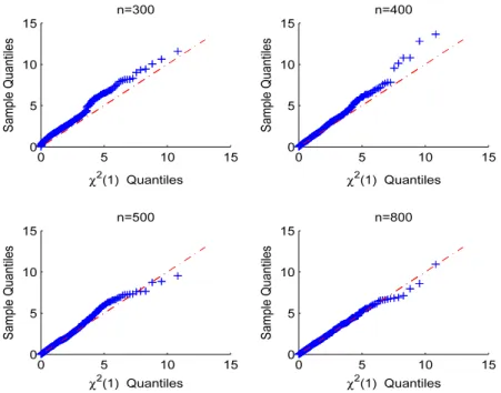
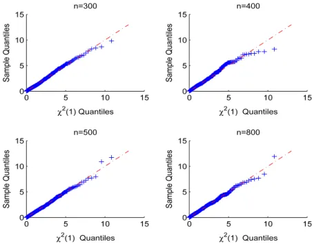
increased.

Figs. 2and3show the QQ plot of Score test statistics and

χ

2distribution. From the two figures, we find the Score test statistics is very close to

χ

2

₍

₁

₎

_{distribution when the sample size increases.}

Meanwhile, as suggested by Chen [3], the power function and the exponential function are usually employed in practice, the score test statistic is not very sensitive to the functional form in the test for homogeneity of variance parameter. This fact might be also true in our above simulation studies.

However, when the sample size is small, especiallynsmaller than 200, we find that the convergence is not very good and the difference between empirical distribution function ofSCtest statistics and

χ

2

₍

₁

₎

_{distribution function is obvious for the}

PLSIBM, which is different from the parametric linear beta regression model [9]. The power of test of the parametric linear beta regression model with varying dispersion is very good when the simulation sample size achieves 40. There may be some reasons causing this problem. Though the single-index estimation decreased the number of the parameters which need to estimate in the PLSIBM, the number of parameters is still not small based on P-spline estimate, which is the sum ofdim

(α)

anddim

(δ)

. Moreover, there are some approximations in the process of estimating and the algorithm given in Section2 depended on the starting value. We conclude that the test statistics does not approximately follow

χ

2

₍

₁

₎

_{distribution when}

Fig. 2. QQ plot underH0with different sample sizes in Case (1). Table 3

Simulated sizes and powers ofSCin Case (1).

n 300 400 500 800 1000 ρ=0 0.063 0.060 0.059 0.055 0.052 ρ=0.1 0.054 0.072 0.078 0.083 0.098 ρ=0.3 0.075 0.125 0.177 0.250 0.352 ρ=0.5 0.143 0.174 0.315 0.417 0.682 ρ=0.7 0.252 0.483 0.573 0.640 0.821 ρ=0.9 0.296 0.512 0.695 0.912 0.973 Table 4

Simulated sizes and powers ofSCin Case (2).

n 300 400 500 800 1000 ρ=0 0.056 0.054 0.045 0.052 0.053 ρ=0.2 0.105 0.130 0.189 0.296 0.404 ρ=0.4 0.269 0.327 0.418 0.604 0.748 ρ=0.6 0.453 0.640 0.824 0.905 0.961 ρ=0.8 0.782 0.875 0.928 0.984 0.996 ρ=1.0 0.906 0.945 0.983 1.000 1.000 5. Concluding remarks

In this paper, we propose the penalized likelihood estimator and score test for the varying dispersion parameter in the framework of PLSIBM. The performance of penalized likelihood estimator and the properties of the score statistic are investigated and examined by Monte Carlo simulations. In practice, the score tests are particularly appealing, because one needs only to calculate statistics under the null hypothesis which is that of the basic model under discussion. Simulation study indicates that the estimator and the test are effective when the sample size is large.

Acknowledgment

The authors would like to thank the referee for his/her valuable comments that led to a greatly improved presentation of the paper.

Appendix

Regularity conditions

Fig. 3. QQ plot underH0with different sample sizes in Case (2).

Assumption 2. The true parameter vector

θ

0is an interior point ofΘ.

Assumption 3. In a neighborhood of

θ

0, Ω

(θ

0

)

=

lim n 1 n n

−

i=1

∂

li

(θ)

∂θ

j



∂

li

(θ)

∂θ

k



T











_θ =θ0

exists and is nonsingular. 1 n n

−

i=1

∂

li

(θ)

∂θ

j



∂

li

(θ)

∂θ

k



T and 1 n n

−

i=1

∂

2_l i

(θ)

∂θ

j

∂θ

k

,

converge uniformly in

θ

in a neighborhood of

θ

0.

Further there exists functionHjkssuch that









∂

3_l

_(θ)

∂θ

j

∂θ

k

∂θ

s









≤

Hjks for all the

θ

wherehjks

=

Eθ0

(

Hjks

) <

∞

forj

,

k

,

s,l

(θ)

=

∑

n i=1li

(θ)

.

Assumption 4.

λ

n

=

o

(

n−1/2

)

.

By the above assumptions, the consistence and asymptotic normality in Section2.3can be established.

Proof of Theorem 1. We now study the asymptotic distribution ofSC underH0. Let

τ

be defined on a compact subset Θ,

τ

ˆ

=

(

ρ,

ˆ

α

ˆ

T

_,

_β

ˆ

T

_,

_δ

ˆ

T

_,

_φ)

ˆ

_{be the penalized likelihood estimate of parameter}

_τ

_{without constraint, and let interior point}

τ

0

=

(ρ

T0

, α

T 0

, β

T 0

, δ

T

0

, φ

0

)

inΘbe the true value of

τ

underH0respectively.

By theAssumptions 2and4, for an arbitrary point

τ

in a neighborhood of

τ

0, we have,

n−1I

(τ)

→

J

(τ

0

) >

0

,

(13)

asn

→ ∞

, uniformly, whereI

(τ)

defined by Eq.(9),J

(τ

0

)

is positive definite at

τ

=

τ

0.

For the notation simplicity, we write

1

τ

ˆ

,

τ

ˆ

− ˆ

τ

₀

=

(

1

ρ,

ˆ

1

θ

ˆ

T

)

T

,

Q

(τ)

,Qn,λn

(τ),

˙

Q

(τ)

=

∂

Q

(τ)

∂τ

=

(

Q

˙

ρ

(τ),

Q

˙

θ

(τ)

T

)

T

,

A standard Taylor expansion ofQ

˙

(τ)

at

τ

ˆ

about

τ

ˆ

₀gives

˙

Q

(

τ)

ˆ

= ˙

Q

(

τ

ˆ

₀

)

+

∂

2_Q

₍

_τ

_ˆ

0

)

∂τ∂τ

T 1

τ

ˆ

+

Op

(

1

).

SinceQ

˙

(

τ)

ˆ

=

0 andQ

˙

_θ

(

τ

ˆ

₀

)

=

0, we have

˙

Q

(

τ

ˆ

₀

)

=

[

_˙

Q_ρ

(

τ

ˆ

₀

)

0

]

=

[

I_ρρ

(

τ

ˆ

₀

)

I_ρθ

(

τ

ˆ

₀

)

I_θρ

(

τ

ˆ

₀

)

I_θθ

(

τ

ˆ

₀

)

] [

1

ρ

ˆ

1

_θ

ˆ

]

+

Op

(

1

).

Correspondingly,

˙

Q_ρ

(

τ

ˆ

₀

)

=

I_ρρ

(

τ

ˆ

₀

)

1

ρ

ˆ

+

I_ρθ

(

τ

ˆ

₀

)

1

θ

ˆ

+

Op

(

1

),

and I_θρ

(

τ

ˆ

₀

)

1

ρ

ˆ

+

I_θθ

(

τ

ˆ

₀

)

1

θ

ˆ

+

Op

(

1

)

=

0

.

By simple algebraic calculations,

˙

Q_ρ

(

τ

ˆ

₀

)

= [

Iρρ

(

τ

ˆ

₀

)

]

−11

ρ

ˆ

+

Op

(

1

).

Then we obtain 1

√

n

˙

Q_ρ

(

τ

ˆ

₀

)

=

n−1

[

Iρρ

(

τ

ˆ

₀

)

]

−1

√

n1

ρ

ˆ

+

Op

(

n−1/2

).

By the Eq.(13), we have

n−1

[

Iρρ

(

τ

ˆ

₀

)

]

−1

−→ [

Jρρ

(

τ

ˆ

₀

)

]

−1

.

Since

τ

ˆ

₀

−→

p

τ

₀,

√

n1

ρ

ˆ

−→

d N

(

0

,

Jρρ

(τ

0

))

. It follows that 1

√

n

˙

Q_ρ

(

τ

ˆ

₀

)

−→

d N

(

0

,

[

Jρρ

(τ

0

)

]

−1

).

Furthermore, sincedim

(ρ)

=

k, we get

SC

=





1

√

n

∂

Q

(τ)

∂ρ



T

(

nIρρ

(τ))



1

√

n

∂

Q

(τ)

∂ρ





ˆ τ0

= {

φ

2fTMIρρMTf

}|

_τˆ0

,

which converges in distribution to a chi-squared distribution withkdegree of freedom asn

→ ∞

.

References

[1] A. Branscum, W. Johnson, M. Thurmond, Bayesian beta regression: application to household expenditure data and genetic distance between foot-and-mouth disease viruses, Australian and New Zealand Journal of Statistics 49 (3) (2007) 287–301.

[2] R. Carroll, J. Fan, I. Gijbel, M. Wand, Generalized partially linear single-index models, Journal of The American Statistical Association 92 (1997) 477–489. [3] C. Chen, Score test for regression models, Journal of The American Statistical Association 78 (1983) 158–161.

[4] R. Cook, S. Weisberg, Diagnostics for heteroscedasticity in regression, Biometrika 70 (1983) 1–10. [5] D. Cox, D. Hinkley, Theoretical Statistics, Chapman and Hall, London, 1974.

[6] P. Espinheira, S. Ferrari, F. Cribari-Neto, On beta regression residuals, Journal of Applied Statistics 35 (2008) 407–419.

[7] P. Espinheira, S. Ferrari, F. Cribari-Neto, Influence diagnostics in beta regression, Computational Statistics and Data Analysis 52 (9) (2008) 4417–4431. [8] J. Fan, I. Gijbels, Local Polynomial Modelling and its Application, Chapman and Hall, New York, 1996.

[9] S. Ferrari, F. Cribari-Neto, Beta regression for modeling rates and proportions, Journal of Applied Statistics 31 (2004) 799–815. [10] W. Härdle, E. Mammen, Testing parametric versus nonparametric regression, Annals of Statistics 21 (1993) 1926–1947.

[11] W. Härdle, T.M. Stocker, Investigating smooth multiple regression by the method of average derivatives, Journal of the American Statistical Association 84 (1989) 986–995.

[12] P. McCullagh, J. Nelder, Generalized Linear Models, 2nd ed., Chapman and Hall, London, 1989.

[13] D. Ruppert, Selecting the number of knots for penalized splines, Journal of Computational and Graphical Statistics 11 (2002) 735–757. [14] D. Ruppert, R. Carroll, Spatially-adaptive penalties for spline fitting, Australian and New Zealand Journal of Statistics 42 (2000) 205–223. [15] J. Wang, L. Xue, L. Zhu, Y. Chong, Estimation for a partial-linear single-index model, The Annals of Statistics 38 (2010) 246–274.

[16] B. Wei, J. Shi, W. Fung, Y. Hu, Testing for varying dispersion in exponential family nonlinear models, Annals of the Institute of Statistical Mathematics 50 (1998) 277–294.

[17] F. Xie, B. Wei, Influence analysis for count data based on generalized poisson regression models, Statistics 43 (1) (2009) 1–20.

[18] Y. Yu, Penalized spline estimation for Generalized partially linear single-index models, 2009 (work paper,http://www.business.uc.edu/Yan-Yu). [19] Y. Yu, D. Ruppert, Penalized spline estimation for partially linear single-index models, Journal of the American Statistical Association 97 (2002)

1042–1054.

[20] L. Zhu, L. Xue, Empirical likelihood confidence regions in a partially linear single-index model, Journal of the Royal Statistical Society, Series B 68 (2006) 549–570.