Model Fit Diagnostics for Hidden Markov Models

(1)

to recognize that its copyright rests with its author and that no quotation from the thesis and no information derived from it may be published without the author’s prior consent.

(2)

(3)

by

Safaa K. Kadhem

A thesis submitted to Plymouth University in partial fulfillment of the

requirements for the degree of

DOCTOR OF PHILOSOPHY

School of Computing, Electronics and Mathematics

Faculty of Science and Engineering

Plymouth University

(4)

(5)

Safaa K. Kadhem

Abstract

Hidden Markov models (HMMs) are an efficient tool to describe and model the underlying behaviour of many phenomena. HMMs assume that the observed data are generated independently from a parametric distribution, conditional on an unobserved process that satisfies the Markov property. The model selection or determining the number of hidden states for these models is an important issue which represents the main interest of this thesis. Applying likelihood-based criteria for HMMs is a challenging task as the likelihood function of these models is not available in a closed form. Using the data augmentation approach, we derive two forms of the likelihood function of a HMM in closed form, namely the observed and the conditional likelihoods. Subsequently, we develop several modified versions of the Akaike information criterion (AIC) and Bayesian information criterion (BIC) approximated under the Bayesian principle. We also develop several versions for the deviance information criterion (DIC). These proposed versions are based on the type of likelihood, i.e. conditional or observed likelihood, and also on whether the hidden states are dealt with as missing data or additional parameters in the model. This latter point is referred to as the concept of focus. Finally, we consider model selection from a predictive viewpoint. To this end, we develop the so-called widely applicable information criterion (WAIC). We assess the performance of these various proposed criteria via simulation studies and real-data applications.

In this thesis, we apply Poisson HMMs to model the spatial dependence analysis in count data via an application to traffic safety crashes for three highways in the UK. The ultimate interest is in identifying highway segments which have distinctly higher crash rates. Selecting an optimal number of states is an important part of the interpretation. For this purpose, we employ model selection criteria to determine the optimal number of states. We also use several goodness-of-fit checks to assess the model fitted to the data. We implement an MCMC algorithm and check its convergence. We examine the sensitivity of the results to the prior specification, a potential problem given small sample sizes. The Poisson HMMs adopted can provide a different model for analysing spatial dependence on networks. It is possible to identify segments with a higher posterior probability of classification in a high risk state, a task that could prioritise management action.

(6)

(7)

List of Figures

2.1 Plot of a mixture density of two univariate Normal components with equal weight proportions, common variance σ2=1, and a fixed mean for the first

component, µ1=0, and different values for the mean of second component,

µ2=i, namely; (a)i=1; (b)i=2; (c)i=3; (d)i=4. . . 39 2.2 Fitting a two-component Normal mixture model using the EM algorithm. . . . 43 2.3 Trace-plots, histograms and ACF functions of all posterior parameters of the

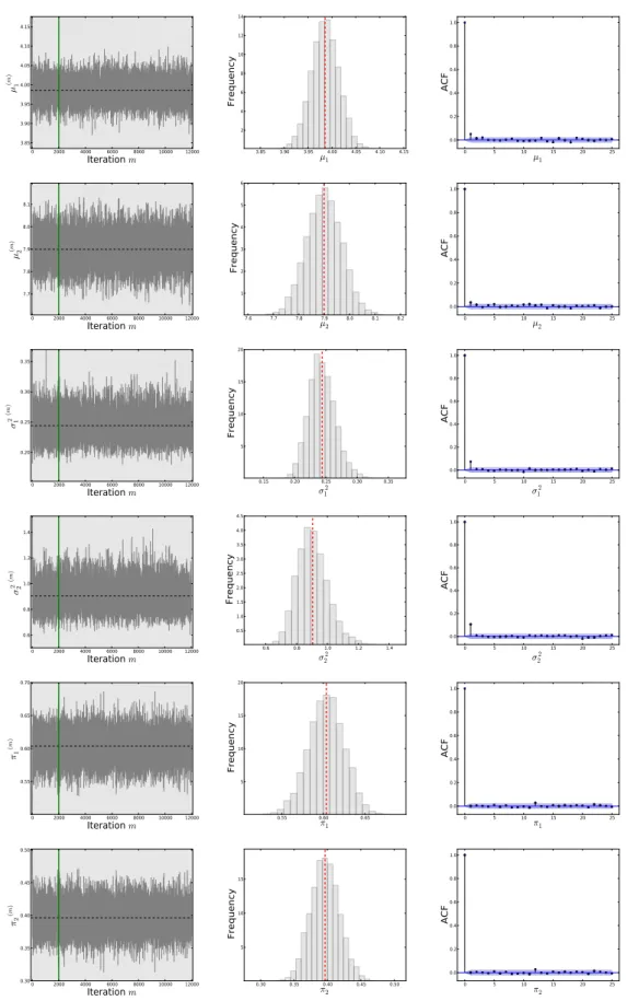
model with the weights:π1=0.7 andπ2=0.3. . . 52 2.4 Trace-plots, histograms and ACF functions of all posterior parameters of the

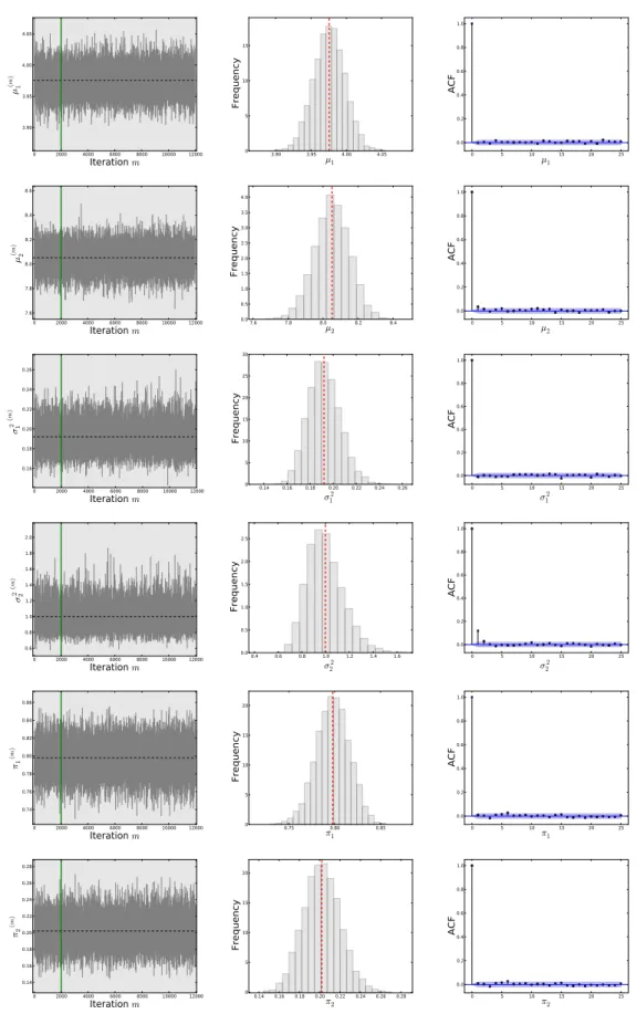
model with the weights:π1=0.9 andπ2=0.1. . . 57 2.9 Fitting of predictive density of all model to synthetic sets of length 500

observation based on the two-component Normal mixture with true weights as labelled in the title each figure. . . 58 2.10 A two-component Normal mixture model fitted to the Acidity data.. . . 60

3.1 Graphical representation of the dependence structure of a discrete-time finite state-space HMM.. . . 65

(16)

3.2 A sequence of observations, of length (T=200), generated from 2-state Normal HMM in the top and the corresponding sequence of hidden states with the same length in the bottom. . . 69 3.3 A sequence of observations, of length (T=200), generated from 3-state Normal

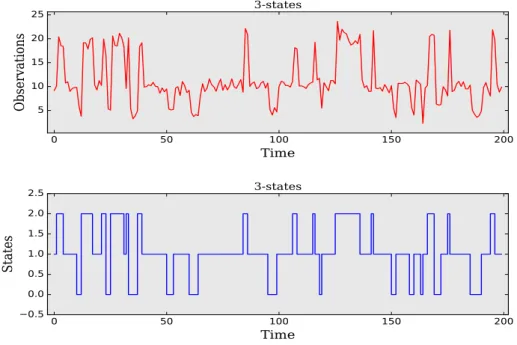
HMM in the top and the corresponding sequence of hidden states with the same length in the bottom. . . 70 3.4 A sequence of observations, of length (T=200), generated from 2-state Poisson

HMM in the top and the corresponding sequence of hidden states with the same length in the bottom. . . 70 3.5 A sequence of observations, of length (T=200), generated from 3-state Poisson

HMM in the top and the corresponding sequence of hidden states with the same length in the bottom. . . 71 3.6 The computational operations required for computing the forward variableαt(j). 76

3.7 The computational operations required for computing the backward variable

βt(j). . . 77

4.1 A Graphical model of the prior distributions and hyper-parameters relevant to the main parameters of a Bayesian HMM. . . 89 4.2 Label switching of Galaxy data fitted to 6-state Normal HMM using the

unconstrained DG sampler. . . 103 4.3 Using the IC method to solve the label switching for a Normal HMM with six

states fitted to the Galaxy data. . . 104 4.4 A histogram of the synthetic data generated from a Normal HMM with 3 states. 105 4.5 Trace-plots of 10 parallel MCMC runs of the mean parameter,µj; j=1,2,3. . 107

4.6 Trace-plots of 10 parallel MCMC runs of the variance parameter,σ2j; j=1,2,3. 107

4.7 Trace-plots of 10 parallel MCMC runs of the initial distribution parameter,

πj; j=1,2,3. . . 108

4.8 Trace-plots of 10 parallel MCMC runs of the probability transition parameters, ajk; j,k=1,2,3. . . 109

(17)

4.9 The graphs show simulations from the posterior distribution of the mean parameter µk; k =1,2,3, of 3-state Normal HMM. The graphs in the first

column represent the trace-plots of the mean parameters (µ1−µ3). The

vertical green line in the trace-plots separates the burned-in samples (M=1000) from those used for the future inference (M=9000), and the horizontal black dashed line shows the true parameter. The graphs in the second column show the histograms of the densities of the mean parameters(µ1−µ3). The black

solid and red dashed vertical lines show the true parameter and posterior mean respectively. The graphs in the third column show the autocorrelation

functions of the mean parameters(µ1−µ3). . . 112

4.10 Fitting the densities of a Normal HMM with 3 states to the synthetic data using the DG sampler. . . 113

4.11 The waiting times between successive eruptions of the Old Faithful geyser.. . . 114

4.12 Sample ACF of the waiting times of the Old Faithful geyser data. . . 114

4.13 Trace-plots of the mean parameter, µj, of 3-state Normal HMM fitted to the waiting times of the Old Faithful geyser data. . . 115

4.14 Trace-plot of the most frequent hidden state sequence (Top). State-dependent means (dashed horizontal points) vs. observations, depicted by the most likely state sequence (Bottom). . . 118

5.1 The graphical representation of the parameters of HMM. . . 131

6.1 Simulated data from 200 Normal HMMs of length 500 withK0=2. . . 163

6.5 Histograms of the densities for several Normal HMMs, with different states, fitted to the waiting time of Old Faithful geyser data. . . 177

7.1 Plots of the M5, M6 and M42 motorways in the UK. . . 184 7.2 Plot of observed crash counts and rates at the segment level of the M5 highway. 185

(18)

7.3 Plot of observed crash counts and rates at the segment level of the M6 highway. 185 7.4 Plot of observed crash counts and rates at the segment level of the M42 highway.186 7.5 The plots of ACF functions of the crash rate parameterλj of a 2-state PHMM

given priors: (A): Gamma(0.1,0.1), (B): Gamma(0.01,0.01), (C):

Gamma(0.001,0.001), (D):Gamma(0.0001,0.0001). . . 194

7.6 The plots of ACF functions of the crash rate parameterλj of a 3-state PHMM

Gamma(0.001,0.001), (D):Gamma(0.0001,0.0001). . . 194

with priors: (A): Gamma(0.1,0.1), (B): Gamma(0.01,0.01), (C):

Gamma(0.001,0.001), (D):Gamma(0.0001,0.0001). . . 195

with priors: (A): Gamma(0.1,0.1), (B): Gamma(0.01,0.01), (C):

Gamma(0.001,0.001), (D):Gamma(0.0001,0.0001). . . 196

7.9 Trace plots for the thinned samples of state-dependent crash rate parameters,

λj;j=1,2,3, sampled from a 3-state PHMM under aGamma(0.1,0.1)prior. . 197

7.10 Box-plots of the estimates of the crash rate parameterλj for a 2-state PHMM

Gamma(0.001,0.001), (D):Gamma(0.0001,0.0001). . . 199

Gamma(0.001,0.001), (D):Gamma(0.0001,0.0001). . . 200

Gamma(0.001,0.001), (D):Gamma(0.0001,0.0001). . . 202

Gamma(0.001,0.001), (D):Gamma(0.0001,0.0001). . . 204

7.14 The posterior predictive distribution with 95% predictive intervals simulated from a 2-state PHMM vs observed crash counts (M5 data). . . 208

(19)

7.15 The posterior predictive distribution with 95% predictive intervals simulated from a 3-state PHMM vs observed crash counts (M5 data). . . 209 7.16 The posterior predictive distribution with 95% predictive intervals simulated

from a 4-state PHMM vs observed crash counts (M5 data). . . 210 7.17 The posterior predictive distribution with 95% predictive intervals simulated

from a 5-state PHMM vs observed crash counts (M5 data). . . 211 7.18 Normal QQ-plots of ordinary pseudo-residuals for crashes data under 2, 3, 4

and 5-state PHMM (M5 data). . . 212 7.19 The ACF plots of the crash rate parameter,λ, of a PHMM with K=2, ...,6,

given a less diffuse prior,Gamma(0.1,0.1), fitted to the M6 data. . . 214 7.20 Box-plots of the posterior distributions of state-specific crash rate parameters of

a PHMM withK=2, ...,6, fitted to the M6 motorway data. . . 216 7.21 The posterior predictive distribution with 95% predictive intervals simulated

from a 6-state PHMM vs observed crash counts (M6 data). . . 223 7.26 Normal QQ-plots of ordinary pseudo-residuals for crashes data under a PHMM

withK=2, ...,6 (M6 data). . . 224 7.27 The ACF plots of the crash rate parameter,λ, of a PHMM withK=2,3 and 4,

given a less diffuse prior,Gamma(0.1,0.1), fitted to the M42 motorway data. . 225 7.28 Box-plots of the posterior distributions of state-specific crash rate parameters of

(20)

7.29 The posterior predictive distribution with 95% predictive intervals simulated

from a PHMM with statesK=2, 3 and 4 vs observed crash counts. . . 230

7.30 Normal QQ-plots of ordinary pseudo-residuals obtained from a PHMM with K=2, 3 and 4 of the M42 motorway data. . . 231

7.31 Trace-plots of the posterior probabilities of hidden states for the 3-state Poisson HMM for the M5 motorway. . . 232

7.34 Trace-plot of the most frequent hidden state sequence (Top). State-dependent crash rates of each segment (dashed line) of the M5 motorway, depicted by the most likely state sequence (Bottom). . . 234

7.37 The spatial results mapped at segment level for the M5 motorway. . . 237

7.38 The spatial results mapped at segment level for the M6 motorway. . . 238

(21)

List of Tables

2.1 The true and estimated values of a two-component Normal mixture model using EM algorithm for a simulated sample of 1000 observations. . . 43 2.2 Results of the parameter estimation of all two-components Normal mixture

models. All models were fitted independently to data set of length T =500, each one with a different mixing weight but fixed mean and variance.. . . 51 2.3 Parameter estimates for two-component Normal mixture model fitted to the

Acidity data.. . . 59

4.1 Gelman and Rubin’s statistics,R, for the mean parameters obtained using DG algorithm. Value less than 1.1 suggests that we could assume the convergence of the MCMC chains. . . 106 4.2 Gelman and Rubin’s statistics,R, for the variance parameters obtained using DG

algorithm. Value less than 1.1 suggests that we could assume the convergence of the MCMC chains. . . 106 4.3 Gelman and Rubin’s statistics,R, for the initial parameters obtained using DG

algorithm. Value less than 1.1 suggests that we could assume the convergence of the MCMC chains. . . 106 4.4 Gelman and Rubin’s statistics, R, for the transition parameters obtained using

DG algorithm. Value less than 1.1 suggests that we could assume the convergence of the MCMC chains. . . 106 4.5 Results of the estimation of mean parameterµk; k=1,2,3, with 95% CI. . . . 111

4.6 Results of the estimation of variance parameterσ_k2; k=1,2,3,with 95% CI. . 111

4.7 Results of the estimation of initial state parameterπk; k=1,2,3,with 95% CI. 111

(22)

4.9 The results of the parameter estimates of 3-state Normal HMM using the DG sampler on the waiting times of the Old Faithful geyser data. The last two rows display the results obtained from previous studies. The numbers in brackets represent the corresponding 95% CIs. . . 117

6.1 Percentage of the number of times in which the models with 2–5 states are chosen by each criterion over 200 independent simulation data sets, each of which of length 500 observations, generated from a HMM withK0=2 states. The numbers in brackets indicate numerical standard errors. . . 169 6.2 Percentage of the number of times in which the models with 2–5 states are

chosen by each criterion over 200 independent simulation data sets, each of which of length 500 observations, generated from a HMM withK₀=3 states. The numbers in brackets indicate numerical standard errors. . . 170 6.3 Percentage of the number of times in which the models with 3–7 states are

chosen by each criterion over 200 independent simulation data sets, each of which of length 500 observations, generated from a HMM withK0=5 states. The numbers in brackets indicate numerical standard errors. . . 171 6.4 Percentage of the number of times in which the models with 5–9 states are

chosen by each criterion over 200 independent simulation data sets, each of which of length 500 observations, generated from a HMM withK0=7 states. The numbers in brackets indicate numerical standard errors. . . 172 6.5 Results of the proposed criteria, based on recursive deviances, for the waiting

time of Old Faithful geyser data. . . 175 6.6 Results of the proposed criteria, based on conditional deviances, for the waiting

time of Old Faithful geyser data. . . 175 6.7 Results of the WAIC and the effective number of parameters, based on the

integrated log-pointwise predictive density, applied for the waiting time of Old Faithful geyser data.. . . 176

(23)

7.2 Results of the estimation and convergence of the rate parameter of a 2-state PHMM, given four gamma priors. The third column provides the ergodic posterior means of the rate parameter. The fourth column provides the median and 95% CI. The last two columns include the values of the Gelman-Rubin statistic, ˆR, and the Geweke statistic, ˆG, respectively. . . 198

7.6 Results of the model selection criteria for several PHMMs with K =2, ...,5 fitted to the M5 highway data under four prior choices: Gamma(0.1,0.1),

Gamma(0.01,0.01),Gamma(0.001,0.001)andGamma(0.0001,0.0001). . . . 206

7.7 Results of the estimation and convergence of the crash rate parameter,λ, of a

PHMM withK=2, ...,6, given a less diffuse prior,Gamma(0.1,0.1), fitted to the M6 motorway data. The third column provides the ergodic posterior means of the rate parameter. The fourth column provides the corresponding 95% CI. The last two columns include the values of the Gelman-Rubin statistic, ˆR, and the Geweke statistic, ˆG, respectively. . . 215

(24)

7.8 Results of the model selection criteria for several PHMMs with K =2, ...,6 fitted to the M6 highway data under four prior choices: Gamma(0.1,0.1),

7.9 Results of the estimation and convergence of the crash rate parameter,λ, of a

PHMM withK=2,3 and 4, given a less diffuse prior,Gamma(0.1,0.1), fitted to the M42 motorway data. The third column provides the ergodic posterior means of the rate parameter. The fourth column provides the corresponding 95% CI. The last two columns include the values of the Gelman-Rubin statistic,

ˆ

R, and the Geweke statistic, ˆG, respectively. . . 226 7.10 Results of the model selection criteria for several PHMMs with K =2,3,4

fitted to the M42 highway data under four prior choices: Gamma(0.1,0.1),

(25)

Completing this work would not have been easy were it not for the support and encouragement that was provided by my Director of Studies, Dr Paul Hewson. So, I must thank him and as I am truly indebted to him for his help. Also, I would like to thank Dr Irene Kaimi, as a second supervisor, for her continuous help during my studies. I am so thankful for her reviewing several drafts of this thesis and for her helpful comments. Also, I have to thank my new supervisor, Professor David McMullan, for helping me at the last stages of submission of my thesis and arranging the final examination.

I would like to thank the Iraqi Ministry of Higher Education and Scientific Research and Al Muthanna University for financing the scholarship that has enable me to complete this thesis. Personally, I would also like to thank all my friends, PhD students, in Plymouth and all members of the School of Mathematics and Statistics. Also, I would like to thank all members of Plymouth University.

Finally, I am so thankful for my parents and family who have supported me since my first days of starting my thesis and until this moment.

To my dear friend, Dr. Muhammed Al-Mallah, who passed away before this work was finished. I will never forget you. You will always remain in my memory.

(26)

(27)

At no time during the registration for the degree of Doctor of Philosophy has the author been registered for any other University award. Work submitted for this research degree at Plymouth University has not formed part of any other degree either at Plymouth University or at another establishment.

Relevant scientific seminars and conferences were regularly attended at which work was often presented. One paper has been accepted for publication in refereed journal.

Publications:

Kadhem, S. K., Hewson, P. & Kaimi, I. (2016). Recursive Deviance Information Criterion for the Hidden Markov Model. International Journal of Statistics and Probability, 5(1), 61-78. DOI: http://dx.doi.org/10.5539/ijsp.v5n1p61

Kadhem, S. K., Hewson, P. & Kaimi, I. (2016). Using hidden Markov models to model spatial dependence in a network. (Under review: Spatial Statistics)

Book reviews

Kadhem, S. K. (2017). Handbook of discrete-valued time series by Richard A. Davis, Scott H. Holan, Robert B. Lund, and Nalini Ravishanker,Journal of the Royal Statistical Society A, Volume 180, Issue 2, February 2017, Pages 682-683.

Posters and conference presentations:

Kadhem, S. K. Bayesian Criteria for Model Choice for Hidden Markov Models.International Conference of the Royal Statistical Society. Exeter University, UK, 7-10 Sept. 2015 Conferences and Courses attended:

(28)

. Statistical Computing and Statistical Inference, University of Cambridge, Cambridge, UK, 2013.

. Applied Stochastic Process and Computer Intensive Statistics, Leeds University, Leeds, UK, 2014.

Word count for the main body of this thesis:55456

Signed:

(29)

Introduction

This chapter includes a brief overview of relevant Bayesian theory and the aims and structure of the thesis. In Section1.1, we present the general concepts of Bayesian inference and some related topics such as the prior and posterior specification as well as the use of the sampling MCMC algorithms for simulation based inference. In Section1.2we summarize the aims and the outline of this thesis.

1.1 Bayesian inference

This section reviews the basic principle of the Bayesian approach and also Bayes law. It also considers computational methods which make a Bayesian approach possible. We consider the Markov Chain Monte Carlo (MCMC) approach, the most widely used procedure in Bayesian sampling. In addition, the section considers how to diagnose convergence of an MCMC sampler.

1.1.1 Basics of Bayesian analysis

In general, statistical inference is the process of drawing conclusions about populations or scientific truths from data, y. To conduct statistical inference, we specify a statistical model, characterized by model parameter(s), θ, that explains the data according to a probability distribution. For example, for a single data point, yt, we may assume

yt ∼Pr(yt|θ), (1.1)

wherePr(yt|θ) =L(θ; yt)is a function of an unknown parameter(s)θ, which is also called the

“likelihood” function. Given a sequence of observations, denoted by the vector

y = (y1,y2, ...,yT), the likelihood function of the entire sequence of observations can be

defined as: L(θ;y) =Pr(y|θ) = T

∏

t=1 Pr(yt|θ). (1.2)

(30)

For example, if we assume that observation yt has been generated from a Normal distribution with parametersθ= (µ,σ2)as Pr(yt|θ) =φ(µ,σ2) = 1 √ 2π σ2exp − 1 2σ2(yt−µ) 2 , (1.3)

the likelihood of the entire independent and identically distributed (iid) sample, Pr(y|θ) =

Pr(y1,y2, ...,yT|θ), is L(θ;y) = T

∏

t=1 Pr(yt|θ) = 1 √ 2π σ2 T exp ( − 1 2σ2 T

∑

t=1 (yt−µ)2 ) . (1.4)

Note that the concept of likelihood function in the Bayesian approach has a different meaning from that in the frequentist approach. In Bayesian approach, the likelihood,Pr(y|θ), is viewed as a conditional probability function that varies with datayat fixed values ofθ, whereas in the frequentist approach the likelihood,L(θ;y), is a mathematical function of the parameterθ for fixed data,y(Kroese and Chan,2014, p.228).

Suppose we are interested in making inferences about an unknown quantity, θ. This can be performed using either the frequentist or the Bayesian approach. In a Maximum Likelihood (ML) approach, this is achieved by finding a valueθ =θ∗that maximizes the likelihood ofy with respect toθ, as follows:

∂L(θ;y) ∂ θ =0, which satisfies ∂2L(θ;y) ∂2θ |_θ₌_θ∗ <0. (1.5)

Alternatively, the inference aboutθ can be implemented using the Bayesian approach, when θ is treated as a random variable represented by a probability distribution. This involves the specification of a prior distribution:

θ∼Pr(θ).

According to the Bayes’ theorem, by combining information from the prior distribution and information about the observed data from the likelihood, we can obtain

Pr(θ|y) =Pr(y|θ)Pr(θ)

Pr(y) ∝Pr(y|θ)Pr(θ), (1.6)

where Pr(θ|y), which represents the probability statement about the unknown parameters given the data, is known as theposteriordistribution and forms the core of Bayesian inference

(31)

(Gelman et al., 2014, p.7). Note that the term Pr(y) =∑θPr(θ)Pr(y|θ) for discrete or Pr(y) = R

θPr(θ)Pr(y|θ)dθ in the case of continuous θ, can be viewed as the marginal

probability of observing the data. It behaves as a normalizing constant which ensures that the posterior distribution is a probability distribution and thus integrates of 1 over all values ofθ. The normalizing constant, Pr(y), in Equation (1.6) is generally not of interest as it does not depend on the parameterθ, and thus it can be ignored during parameter estimation.

Many efficient procedures have been proposed for approximating the posterior in Equation (1.6). One of which is known as the Markov chain Monte Carlo (MCMC) method (Geyer, 2011).

1.1.2 The prior distributions

As discussed in Section (1.1.1), the posterior distribution is based on two main components, the likelihood model and the prior distribution. However, the functional form of the prior distribution is often unknown. In this case, the choice of prior is commonly based on assumptions (Carlin and Louis,2009;Gelman et al.,2014). Such assumptions are often based on various factors such as physical considerations, degree of knowledge and, more controversially, mathematical convenience. The choice of prior distribution is an essential part in Bayesian analysis in view of its ability in simplifying the posterior manipulations.

Prior distributions can be classified as informative and non-informative priors. Informative priors are used when prior knowledge is available. On the other hand, the non-informative priors are used when noa prioriknowledge is available. Such priors have a minimal effect on inference as they provide little prior information for the unknown parameters of the model. Hence, the data will be mostly responsible for the posterior distribution, or as described by (Gelman et al.,2014) “to let the data speak for themselves”, so that inference is not affected by external information. Examples of priors intended to be non-informative are flat priors (e.g. that a parameter is uniformly distributed between −∞ and +∞, or between 0 and +∞), reference priors (Berger and Bernardo, 1989) and Jeffreys’s prior (Jeffreys, 1961) which is expressed as Pr(θ)∝|I(θ)| 1 2_, _where _I₍_θ_{) =}−_E −∂2logf(y|θ) ∂ θ0∂ θ .

The termI(θ)is called Fisher’s information matrix and the expectation is taken with respect to the sampling distribution of y. The Jeffreys’ prior gives an automated method for finding a

(32)

non-informative prior for any parametric model. Also, it is known that the Jeffreys’s prior is invariant to transformation.

It is said that the prior is a conjugate prior if the posterior distribution follows the same distribution family as the chosen prior. A common class of distributions that all their members have conjugate priors is the exponential family. The exponential family of distributions can be written as:

Pr(yt|θ) = f(yt)g(θ)exp

φ(θ)0u(yt) . (1.7)

In general, the factorsφ(θ)andu(yt)are vectors of the same dimension asθ. The factorφ(θ)

is called the natural parameter of the exponential family. The likelihood of the whole sequence ofiidvariables, a function ofθ, can be then written as

Pr(y|θ) = n

∏

t=1 f(yt) ! g(θ)Texp ( φ(θ)0 T

∑

t=1 u(yt) ) , (1.8)

which has a fixed form

Pr(y|θ)∝g(θ)Texpφ(θ)0h(y) , (1.9) whereh(y) =∑tn=1u(yt)denotes a sufficient statistic forθ, because the likelihood forθdepends on the datayonly through the value ofh(y). If the prior density is specified as:

Pr(θ)∝g(θ)ηexpφ(θ)0v , (1.10) then the posterior distribution is

Pr(θ|y)∝g(θ)η+Texpφ(θ)0(v+h(y)) , (1.11) which shows that this choice of prior density is conjugate. For the Normal distribution, where variance parameterσ2is known while the mean parameter µ is unknown, the conjugate prior of the unknown mean parameter can take the form of a Normal distribution as

(33)

which leads to the posterior distribution Pr(µ|y,σ2,µ0,σ02)∝exp ( −1 2 1 σ₀2+ T σ2 µ− σ₀2Ty¯+µ σ2 σ₀2σ2 2) , ∼N σ₀2Ty¯+µ σ2 σ₀2σ2 , σ₀2σ2 σ₀2+σ2 , (1.13)

whereT denotes the sample size. In addition to the Normal distribution, there are many widely used distributions that belong to the exponential family, for example, the Poisson, Gamma, Beta, Dirichlet, binomial and Multinomial distributions (Gelman et al.,2014).

1.1.3 Markov Chain Monte Carlo method

The main aim of Bayesian inference is to approximate the posterior distribution, Pr(θ|y), in Equation (1.6), as a function of θ. However, in high–dimensional models, where θ is a multi–dimensional vector, we may often face the problem of obtaining the marginal posterior distribution for a single given parameter such as θi (where 1<θi <k). In principle, the

marginal posterior density ofθiis the integral of the joint posterior density of all elements ofθ except θi. In practice, evaluating such integrals is analytically difficult. It is possible to

evaluate these integrals numerically using Markov Chain Monte Carlo (MCMC) methods, in which a Markov chain is used to sample from the posterior distribution. The main idea behind the MCMC method is that it provides an approximation to the posterior distribution by generating sequentially sampled values, where the posterior distribution depends on its previous sampled value for each unknown parameter (Gelman et al., 2014). The MCMC approach is based on two key aspects, namely, the Markov chain and Monte Carlo integration. So, to understand more about the MCMC methods, it is useful to have a look at these two concepts.

1.1.3.1 Markov chains

The MCMC method works by creating a Markov chain that represents the posterior distribution of interest. A Markov chain can be defined as a particular type of discrete time Markov process,X(t);t≥0 , with state spaceS=sj;j=1,2, ...,K , K6∞. A sequence

X0,X1,X2...of random variables is aMarkov chainif the conditional distribution ofXt+1given

X0, ...,Xt depends only onXt (Geyer,2011). We can write this as

(34)

for all sj,si,sit−1, ... ∈S and t = 0,1,2, .... In other words, the future and past states are

independent, given the current state. This property is called the Markov property. The probability

pi j=Pr(Xt+1=sj|Xt=si); si,sj,∈S, (1.15)

is called the transition probability from statesi to statesj. If there areKpossible states, then

P=pi j; i,j=1,2, ...,K, (1.16)

represents the transition matrix of dimensionK×Kthat provides the various probabilities of all possible moves among these states for everyi,∑Kj=1pi j=1. Letπj(t) =Pr(Xt=sj)denote the

probability that the chain is in statesj at timet, andπ(t) ={π1(t),π2(t), ...,πK(t)}denote the

K-length vector of these state probabilities at timet. The probability that the chain is in statesj

at time (step)t+1 is given by

πj(t+1) =Pr(Xt+1=sj), =

_∑

i Pr(Xt+1=sj|Xt =si)Pr(Xt =si), =

_∑

i pi jπi(t), (1.17)

where Equation (1.17) describes the evolution of the chain using a number of successive iterations. Using matrix notation, Equation (1.17) can be written as

π(t+1)=π(t)P. (1.18)

It follows that

π(t)=π0P(t). (1.19)

The n-step transition probability, p(_{i j}n), is the probability that the chain is in the statesj given

thatnsteps earlier it was in the statesi, i.e.,

(35)

where p(_{i j}n) is just thei,jth element of P(n). A Markov chain is said to beirreducibleif there exists a positive integerni j such that p

ni j

i j >0, for alli,j=1,2, ...,K. That is, one can move

from any state to any other state inSpossible states in a finite number of steps.

A state in a Markov chain is classified asabsorbing,transient, orrecurrentto characterize how often the state is visited or the time between visits. Let f_{i j}(n)denote the probability that the chain first visits the statesjat stepn, when it started in the statesiat step 0, i.e.,

f_{i j}(n)=Pr(X1=6 sj,X26=sj, ...,Xn−16=sj,Xn=6 sj|X0=si), (1.21)

with f_ii(0)=1 and f_{i j}(0)=0 for j6=i. Further, define the sum of probabilities of the first visiting times beingn=1,2, ..., fi j= ∞

∑

n=1 f_{i j}(n), (1.22)

which is the probability that the chain visits state sj in finite time if it starts in state si. In

particular, fiiis the probability of returning to the starting statesiin finite time. A statesjis said

to be: transient if fj j<1, recurrent if fj j=1, and absorbing if pj j=1. If statesj is recurrent,

then it is said to be positive recurrent if the mean time between revisits is finite, i.e.,

∞

∑

n=1

n f(_{j j}n)<∞. (1.23)

Otherwise, it is said to benull recurrent. If one state in an irreducible Markov chain is positive recurrent, then all the states are positive recurrent. The period of a statesjis defined as

dj=gcd

n

n≥1|p(_{j j}n)>0 o

, (1.24)

wheredj denotes the greatest common divisor (gcd) of all integersn≥1. It can be shown that

for an irreducible Markov chain,dj=d,∀j. Ifd>1, the chain is said to beperiodicwith period

d. Ifd=1, then the chain is said to beaperiodic, which means that the chain is not forced into some cycle of fixed length between certain states. It can be seen that ifPhas no eigenvalues equal to 1 the chain is aperiodic. The limiting probability limn→∞p

(n)

j j may or may not converge.

For a transient or null recurrent statesj, limn→∞p

(n)

j j =0, i.e., the probability of the chain being

in statesjeventually goes to zero. If statesjis positive recurrent and periodic, then limn→∞p

(n)

j j

will not converge. Ifsj is positive recurrent and aperiodic, then limn→∞p

(n)

j j will converge to a

(36)

stationary distributionπ, where the vector of probabilities of being in any particular given state is independent of the initial conditionπ(0). The stationary distribution satisfies

π=πP. (1.25)

A sufficient condition for a unique stationary distribution is that the detailed balance or time reversibility condition, namely,

πipi j=πjpji; ∀i,j, (1.26)

is satisfied. Indeed, reversibility of a Markov chain for a desired distribution π implies that the Markov chain has π as its stationary distribution. Given a Markov chainX1, X2, ..., the

transition probability distribution is said to be reversible regarding an initial distribution if the distribution of pairs (Xt,Xt+1) is exchangeable. Reversible Markov chain plays a main role

in MCMC methods (Fan and Sisson, 2011). Given a reversible Markov chain Xm with the

stationary distributionπ, it follows that 1 M M

∑

m=1 h(Xm)−→ Z h(x)π(x)dx, as M−→∞, (1.27) which links Markov chains to Monte Carlo methods, wherem=1,2, ...,M, is a desired period of iterations. Now, it is easy to calculate the posterior quantities using Equation (1.27) because the stationary distributionπis equal to the posterior densityPr(θ|y).

1.1.3.2 Monte Carlo integration

In practice, inference usually requires the integration of posterior distribution over the parameter space. However, for complicated models, such integration is difficult or impossible to be achieved analytically. For this reason, Monte Carlo integration is often utilized to approximate such integrals (Rizzo,2008).

For example, assume one is interested in computing the expectation of some function hof a random variableY that has probability density function fY(y):

E[h(Y)] = Z

h(y)d fY= Z

(37)

Hence, an approximation to this integral can be computed by estimating the sample average of random variables y1,y2, ...,yT drawn from the distribution ofY as follows

d h(y) = 1 T T

∑

t=1 h(yt). (1.29)

It follows that the estimatehd(y)is a strongly consistent estimate of E[h(Y)], such thathd(y)−→ E[h(Y)]as the sample sizeT−→∞. Consequently, it can be said thathd(y)converges to E[h(Y)] with probability 1 asT −→∞. Also, according to the Central Limit Theorem,

d h(y)−E[h(Y)] σ/ √ T −→φ(0,1) asT−→∞, (1.30) whereσ/ √

T is the standard error of estimatehd(y)and_σ2=Var(h(Y))is variance of sample. The main idea of applying the Monte Carlo approach is obtaining the solution of integrals which involve the posterior distributionPr(θ|y)mentioned earlier in Equation (1.6).

1.1.4 MCMC sampling techniques

Markov chain Monte Carlo (MCMC) methods are a framework that involves many techniques introduced byMetropolis et al.(1953) andHastings(1970) for Monte Carlo integration. In this section, we review the well-known Metropolis-Hastings and Gibbs algorithms.

1.1.4.1 The Metropolis-Hastings algorithms

Metropolis-Hastings algorithms (M-H) are a class of Markov Chain Monte Carlo (MCMC) methods. M-H algorithms include many special algorithms such as: the Metropolis Sampler, the independent sampler, the random walk sampler and the Gibbs sampler. The main idea here is to generate a Markov chain{Xt;t=0,1,2, ...}, such that its stationary distribution is the target

distribution. This chain must satisfy the regularity conditions discussed in the previous section, i.e. irreducibility, positive recurrence and aperiodicity. In general, the algorithm must specify how to generate the next state Xt+1, given state Xt. The M-H algorithms assume candidate

valuesY that can be generated from some proposal distributiong(.|Xt). If the candidate point is

accepted, the chain moves to stateY at timet+1 andXt+1=Y; otherwise the chain stays in state

Xt andXt+1=Xt. The choice of proposal distribution is very flexible, but, the chain selected

must meet the regularity conditions. Choosing proposal distributions with the same support set as the target distribution will usually satisfy those the regularity conditions (Rizzo, 2008). A Metropolis-Hastings algorithm associated with target density f and conditional density g

(38)

produces a Markov chain, X(t); see algorithm (1). The conditional distributiongis called the Algorithm 1: Metropolis-Hastings algorithm

Given x(t), 1. GenerateYt ∼g(y,x(t)). 2. Take X(t+1)= ( Yt with probabilitya(x(t),Yt) x(t) _{with probability 1}₋_a₍_x(t)_,_Y t). where; a(x,y) =min 1, f(y) f(x) g(x|y) g(y|x) .

3. Stop when convergence is achieved.

proposal density, the ratioa(x,y)is called theHastings ratiooracceptance probabilityand the step (2) in the algorithm is calledMetropolis rejection. This algorithm always accepts values yt

such that the ratio f(yt)

g(yt|x(t))

is increased, compared with the previous value f(x (t)₎

g(x(t)_|_y

t)

. In this algorithm, the chain convergence largely depends on the proposal density. A proposal density with large jumps to places far from the support of the posterior has low acceptance rate and causes the Markov chain to stand still most of the time. On the other hand, a proposal density with small jumps and high acceptance rate may cause the chain to move slowly and to get stuck in one state. Also, in multi-dimensional cases, the M-H algorithm as described above might require a proposal density for the whole vector, which is extremely difficult when the dimension is high (Casella and Robert,2004).

1.1.4.2 The Gibbs sampler

Gibbs sampler is a special case of the M-H algorithm. Sampling using the Gibbs sampler was proposed by Geman and Geman (1984). This sampler is often applied when the target distribution is multivariate. It regards that all the univariate conditional densities in a multivariate distribution can be specified and that they are easy to sample from. The chain is generated by successively sampling from the conditional distributions of the target distribution (Rizzo,2008, p.263).

A Gibbs sampler generates a sample from the distribution of each parameter or variable conditioning on the current values of the other parameters or variables. As a simplified example, given an multivariate probability distribution, θ= (θ1, ...,θd), we define the d−1

(39)

dimension random vectors

θ(−j)= (θ1, ...,θj−1,θj+1, ...,θd), (1.31)

and denote the corresponding univariate conditional density ofθjgivenθ−jby f(θj|θ−j). The

Gibbs sampler generates the chain by sampling from each of the densities f(θj|θ−j). Algorithm

(2) summarizes the steps of sampling using Gibbs sampler (Marin and Robert,2014, p.90). Algorithm 2: General Gibbs Algorithm

I- Initialization: Start with an arbitrary valueθ(0)_{= (}

θ₁(0), ...,θ_d(0)). II- Iterationt: Given(θ₁(t−1), ...,θ_d(t−1)), generate:

1-θ₁(t)according to f1(θ1|θ₂(t−1), ...,θ_d(t−1)), 2-θ₂(t)according to f2(θ2|θ₁(t),θ₃(t−1), ...,θ_d(t−1)),... d-θ_d(t)according to fd(θd|θ (t) 1 ,θ (t) 2 , ...,θ (t) d−1) 1.1.5 Convergence of MCMC methods

MCMC methods have to be carefully implemented. It is important to check that the algorithm explore the posterior distribution fully and that the simulation converges the posterior distribution (Gelman et al., 2014). Some specific implementations are used to check the algorithm include the deciding when to stop sampling or the required length of sampling, the length of burn-in sample that should be discarded and whether a Markov chain has mixed sufficiently. Indeed, there is no single test or diagnostic tool that correctly checks convergence (Gelman et al., 2014). Consequently, many different techniques have been developed, each with a range of advantages and disadvantages, as tools to check convergence. Some of those techniques are claimed to perform well with the M-H algorithm, others are claimed to perform well with the Gibbs sampler (Cowles and Carlin,1996). Convergence can be diagnosed based on visual methods, including trace density, trace mean, and autocorrelation plots, or using test statistics such asGelman and Rubin(1992),Geweke(1992) andRaftery and Lewis(1992). We will consider the following convergence tools.

(40)

Gelman-Rubin statistic ( ˆR, (Gelman and Rubin,1992)):

The Gelman-Rubin statistic is based on running multiple chains with different over-dispersed starting points. These chains are then compared by calculating the within chain varianceWand between chain variance B. GivenW andB, the estimated marginal posterior variance ofθ is computed as d Var= (1−1 n)W+ ( 1 nB),

wherenis the number of samples drawn. The statistic assesses whetherW andBare different enough to worry about convergence. We then compute the estimated scale reduction using

ˆ R= s d Var W .

BothVardandWare expected to converge to the true marginal posterior variance. Hence, values of ˆR close to 1 (and often less than 1.1) are considered as an evidence that the chains have converged (Gelman and Hill,2007, p.358).

Geweke statistic proposed byGeweke(1992):

This statistic is based on a single chain. After discarding a desired burn-in period, Geweke’s statistic depends on comparing the difference between the means of the first 10% and 50% of chain over aZstatistic that follows asymptotically a standard-normal distribution:

Z= θˆ A₋_ˆ θB s SA_θ TA +S B θ TB ,

where ˆθA and ˆθB denote the means of first and second sample means, respectively,SA_θ andS_θB denote the sample variance corresponding to the first and second part of chain, respectively, and

TAandTBrepresent the sizes of first and second part of chain, respectively. A valueZwithin the

interval[−2,2]denotes no a notable difference between two samples, and hence, convergence is achieved, and vice versa.

Autocorrelation function (ACF):

Because the samples produced by MCMC methods are moving at random small steps which may be correlated, these methods may not be an efficient to represent independent samples of the target distribution (Cowles and Carlin, 1996). Convergence diagnostics can additionally be monitored graphically using the autocorrelation function (ACF) (Ntzoufras,2009;Gelman

(41)

et al.,2014). Given a chain of samples, xm: m=1,2, ...,M,generated from an MCMC method,

the ACF describes the correlation between successive elements xmand xm+1 of the chain at a

different sampling lagsl. The ACF is defined as

ρ(l) =Cov(xm,xm+1) Var(xm) , = ∑ M−1 m=1(xm−¯x)(xm+1−¯x) ∑Mm=1(xm−¯x)2 .

If ACF drops to zero at lag 1, it implies that there is no correlation between successive samples. The ACF is not a convergence diagnostic tool, but can be helpful indirectly to assess convergence of the MCMC algorithms. The MCMC algorithms produce Markov chains of correlated consecutive samples. These correlated samples are then used to summarize many features, e.g. means, variances and percentiles, which assume to be approximated features to the target distribution. However, these approximations are often less accurate than if they were produced from independent samples (Ntzoufras,2009;Gelman et al., 2014). In practice, this autocorrelation between samples is often reduced using the so-calledthinningtechnique. The thinning method is based on keeping only every mth samples after a pre-specified burn-in period is discarded from the posterior distribution. Thus, inference will be adopted mainly on those thinned chains (Ntzoufras,2009;Gelman et al.,2014).

1.2 The aims and outlines of the thesis

The main aim of this thesis is to develop Bayesian diagnostic tools for the model selection issue in a Hidden Markov model context. Under the Bayesian perspective, we develop likelihood-based criteria from the AIC, BIC and DIC for HMMs. We extend the original definition of the DIC taking into account the concept of focus and the availability of closed form of the likelihood of HMMs. We also contribute in developing Bayesian modified versions of the AIC and BIC which approximated at the posterior distribution of the model parameters. We also examine the WAIC (Watanabe,2010), based on the predictive pointwise density. We also develop a Poisson hidden Markov model (PHMM) to spatially model the traffic crash data. Our methodology is illustrated by application involving the crashes which occurred on several motorways in the UK. We are interested in identifying highway segments which have distinct crash rates (distinct states) of the relative safety process. Selecting an optimal number of states is an important part of the interpretation.

(42)

The structure of this thesis is organized as follows:

In Chapter2we present briefly the concept of mixture models to give a better understanding of hidden Markov models.

In Chapter3we include the fundamental definitions and notations of the HMMs. In addition, we introduce the idea of presenting the HMM as a generative model. We develop an algorithm to explain the mechanism of generating data from a parametric HMM. Furthermore, this chapter presents the concept of forward-backward algorithm, as well as the estimation of the model parameters using the EM approach.

Chapter 4 discusses the inference technique for the unknown parameters of hidden Markov models within the Bayesian framework. We set out a theory of hidden state models and develop the necessary MCMC algorithm. We discuss the problem of estimation of the hidden state sequence of a HMM. In addition, this chapter discusses the problem of label switching. We review the literature relevant to this problem and also its solutions.

In chapter5we consider the model selection issue of HMMs. We derive several forms of the likelihood function of a HMM, namely, the observed, complete and conditional likelihood. We develop several conditional and observed likelihood-based versions for the Deviance information criterion (DIC; Spiegelhalter et al., 2002). In addition, we propose several modified versions of the Akaike information criterion (AIC; Akaike,1973) and the Bayesian information criterion (BIC;Schwarz,1978) approximated from a Bayesian perspective. Also, this chapter introduces a criterion based on assessing the predictive ability of a HMM, the widely applicable information criterion (WAIC;Watanabe,2009).

In chapter 6, we introduce simulation studies based on synthetic and real data application to assess the model selection criteria proposed in chapter5.

in Chapter 7 we presents an application involving the traffic crash data. In this chapter we model the spatial dependency, rather than the temporal dependency, on a highway segment using a Poisson hidden Markov model (PHMM). We apply our methodology to identify the highway segments that have distinct crash rates (distinct states) of the relative safety process. This chapter also includes the process of estimation and model selection taking into account the sensitivity analysis of some priors chosen for the state-specific crash rates.

Finally, chapter8dedicated to summarize the work of this thesis and introduce some proposed ideas for future research of HMMs.

(43)

Finite Mixture Models

2.1 Introduction

Hidden Markov models can be considered as an extension of mixture models where the observations are generated independently from some distribution depending on a state or component follows an unobserved Markov process (Cappé et al.,2005). In order to understand the theoretical structure of hidden Markov models, we devote this chapter for reviewing briefly some fundamentals of mixture models. This thesis mainly concentrates on HMMs with a discrete and finite state space.

Mixture models have been developed as a flexible tool to model data with an unobserved heterogeneity, for example, different types of data can form clusters or groups. A finite mixture model (FMM) is generally used when an observation belongs to one of K groups (components) that have distinct features and can be described by different probability distributions (Marin and Robert,2014). In other words, these models are a weighted average of a finite number of distributions (mixing components). In real life, FMMs may be a finite mixture of distributions such as Gaussian or Poisson distributions (McLachlan and Peel,2000; Frühwirth-Schnatter,2006).

Interest in FMMs has increased over the last decades. They can be used for cluster analysis, latent class analysis, discriminant analysis, image analysis, survival analysis, disease mapping and meta analysis. There are many textbooks which have focused in detail on finite mixture models such asMcLachlan and Peel(2000);Frühwirth-Schnatter(2006);Schlattmann(2009); Marin and Robert(2014).

Bayesian methods to model these mixtures of distributions have been used widely for inference. The extensive use of these distributions led to the rapid development in posterior simulation techniques such as MCMC methods (McLachlan and Peel, 2000, p.5). Therefore, MCMC procedures have been used to handle the difficulties in the estimation processes of parameters of FMM such as the number ofkcomponents (Richardson and Green,1997), and

(44)

the effect of label switching (Stephens, 2000; Jasra et al., 2005). Moreover, the Bayesian framework has been employed to simplify these complicated structures by classifying them into a set of simple structures using hidden or latent variables (Marin and Robert,2014). 2.2 Definition of the finite mixture model

One way of conceptualizing the FMM would be to assume that the data arise from a mixture of pre-specified number of sub-populations in different proportions instead of one population. Lety= (y1,y2, ...,yT)denote a sample of observed data with lengthT, the probability density

function (pdf) of a mixture model can be defined as a combination ofKcomponent pdfs

Pr(y|Θ) =

K

∑

k=1

πk Prk(y|θk), (2.1)

wherePrk(y|θk)denotes the pdf of thekthcomponent,πkis the weight of the populationksuch

that 0≤πk≤1, and K

∑

k=1 πk=1,

Θ= (π;θθ) = (π1,π2, ...,πk;θ1,θ2, ...,θk)denotes a set of all unknown weights and parameters

of a mixture model. In many applications, a family of distributions having the density in Equation (2.1) can be called aK-component finite mixture model.

The main idea of mixture model is that the observations y are generated from K distinct random processes, so that each process is modelled by the densityPrk(y|θk), andπkrepresents

the corresponding proportion of observations from this process. For example, consider a FMM where Pr(y|Θ) is constituted from densities which are all Normal distributions. For simplification, assume a mixture of two univariate Normal components with common variance σ2and meansµ1andµ2in proportionsπ1andπ2, so that

φ(yt;Θ) = 2

∑

k=1 πk φk(yt;θk) = 2

∑

k=1 πkφk(yt;µk,σ2) =π1φ1(yt;µ1,σ2) +π2φ2(yt;µ2,σ2), (2.2)

whereΘ= (θk,πk) = (µ1,µ2,σ2;π1,π2)denotes all unknown parameters of a two-component

Normal mixture model, and

φ(yt;µ,σ2) = (2π)− 1 2_σ−1_exp −1 2(yt−µ) 2_/ σ2 , (2.3)

(45)

denotes a univariate Normal density with meanµ and varianceσ2. If the two Normal densities are sufficiently divergent, then the mixture density f(yt)forms a bimodal density. Figure (2.1)

shows a Normal mixture model for various values of µ2 whereµ1=0 andσ₁2=σ₂2=1 with equal weight proportions(π1=π2=0.5). It can be seen that when values ofµ2increase, the

shape of mixture density f(yt)changes from unimodal to bimodal.

(a)

(b)

(c)

(d)

0.40

0.35

0.30

0.25

0.20

0.15

0.10

0.05 0.00 6 4 2 0 2 4 6 8

0.25

0.20

0.15

0.10

0.05 0.00 6 4 2 0 2 4 6 8

0.00 6 4 2 0 2 4 6 8

0.20

0.15

0.10

0.05

0.20

0.15

0.10

0.05 0.00 6 4 2 0 2 4 6 8

Figure 2.1:Plot of a mixture density of two univariate Normal components with equal weight proportions, common varianceσ2=1, and a fixed mean for the first component, µ1=0, and different values for the mean of second component,µ2=i, namely;

(a)i=1; (b)i=2; (c)i=3; (d)i=4.

2.3 Mixture model estimation

Given aniidrandom sample,y= (y1,y2, ...yT), generated from aK-component mixture model

defined in Equation (2.1), the likelihood function of these observations, assuming that yt is

independently distributed, can be written as

Pr(y|Θ) =L(Θ|y) = T

∏

t=1 {π1Pr1(yt;θ1) +π2Pr2(yt;θ2) +...+πKPrK(yt;θk)} = T

∏

t=1 K

∑

k=1 πk Prk(yt|θk). (2.4)

(46)

The maximum likelihood estimator ofΘis defined to be ˆ

Θ=arg max

Θ

L(Θ|y). (2.5)

The main task is to find the parameter vectorΘthat maximizesL(Θ|y). However, the function in Equation (2.4) is difficult to maximize directly as it involves a summation inside the logarithm operator. Additionally, it is not clear which component of the mixture generated each data point and thus which parameters require adjusting to fit that data point. Consequently, a number of methods have been developed for maximizing the log-likelihood function either using the expectation-maximization (EM) or Bayesian methods.

2.3.1 Expectation-Maximization algorithm (EM) of FMMs

One common approach to estimate the parametersΘ= (π,θθ)with respect to the observed data y is by maximizing the likelihood function using Expectation Maximization (EM) algorithm (Dempster et al.,1977). The EM procedure has been used to maximize the likelihood function when there are missing values or latent variables. The key idea of the EM algorithm is the data augmentation procedure (Tanner and Wong, 1987). In the mixture model context, the missing data is represented by a set of random discrete indicatorsz= (z1,z2, ...,zT), where zt∈

{1, ...,K}indicates which mixture component generated the observation yt. Mathematically,

givenz= (z1,z2, ...,zT), the complete-data log-likelihood,Lc(.), can be written as

Lc(Θ|y,z) =Pr(y,z|Θ) =Pr(y|z,Θ)Pr(z|Θ), = T

∏

t=1 K

∏

k=1 {πkPrk(yt|θk)}I(zt=1), = T

∏

t=1 K

∏

k=1 π_kI(zt=1)Prk(yt|θk)I(zt=1), (2.6)

whereI(zt =1) =1 if zt =k holds, wherek=1,2, ...,K, andI(zt =1) =0 otherwise. The

complete log-likelihood,`c(.), as `c(Θ|y,z) = T

∑

t=1 K

∑

k=1 zktlog[πkf(yt;θk)], = T

∑

t=1 K

∑

k=1 zktlogπk+ T

∑

t=1 K

∑

k=1 zktlogf(yt,θk). (2.7)

The key idea behind the EM algorithm is to set an upper bound function Q−function on the negative log-likelihood of the observed variables by introducing distributions over the latent

(47)

variables. The EM algorithm involves two steps to maximize the above log-likelihood which are: Expectation step (E-step) and maximization step (M-step).E-stepincludes the finding the expectation with respect to the conditional distribution of latent variableszgiven data pointsy and the current estimation of parametersΘ(m):

Q(Θ|Θ(m)) =E_z_|₍_y_,_Θ(m)₎[`c(Θ|y,z)]. (2.8)

InM-step, a newΘ=Θ(m+1)is computed, which maximizes the Q-function that is obtained in E-step:

Θ(m+1)=arg max

Θ

Q(Θ|Θ(m)). (2.9)

Initially, the M-step requires the maximization of Q(Θ;Θ(0)) with respect to Θ over the parameter space. This implies choosingΘ(1)such that

Q(Θ(1);Θ(0))>Q(Θ;Θ(0)). (2.10) The E-stepand theM-stepare then implemented again with Θ(0) replaced by the current fit Θ(1). On the(m+1)th iteration theE-stepand theM-stepare alternated repeatedly until the changes in the log-likelihood values are less than some specified threshold, (McLachlan and Peel,2000, p.24). The EM algorithm is numerically stable with each EM iteration increasing the likelihood value as

Q(Θ(m+1))>Q(Θ(m)). (2.11) Before that, we need to define the posterior probability of latent variable zkt. The E-step of the

EM algorithm is carried out by replacing the zkt by their expected values given the datayand

current estimate of the model parameters Θ(m). According to the Bayes theorem (McLachlan and Peel,2000), we obtain

E(zkt|y,Θm) =Pr(zkt=1|yt,Θm) = Pr(yt|zkt=1)Pr(zkt=1) ∑lPr(yt|zlt=1)Pr(zlt =1) = πkf(yt,θk) ∑lπlf(yt,θl) =wkt. (2.12)

(48)

By substituting zktby wkt in Equation (2.7), theE-stepof the EM algorithm is then given as Q(Θ;Θ(m)) =E_Θ(m){`c(Θ|y,z)}, (2.13) = T

∑

t=1 K

∑

k=1 wktlogπk+ T

∑

t=1 K

∑

k=1 wktlogf(yt,θk). (2.14)

TheM-stepinvolves maximization of the current expected complete data likelihood. Sinceπk

appears only in the first term, andθk only in the second term, we can maximize the two terms

separately. To maximize the expression forπk, we introduce the Lagrange multiplierLwith the

constraint that∑Kk=1πk=1, and solve the following equation (Bilmes,1998):

∂ ∂ πk " T

∑

t=1 K

∑

k=1 wktlogπk+L(

∑

k πk−1) # =0 (2.15) or T

∑

t=1 1 πk wkt+L=0. (2.16)

Summing both sides overk, we get thatL=−T resulting in:

π_k(m+1)= 1 T T

∑

t=1 wkt, (2.17) where wkt= πkf(yt,θk) ∑lπlf(yt,θl)

. If the component parameters are unknown, they are estimated by finding the maximum likelihood estimator for the second sum of the expected complete data likelihood: θ_k(m+1)=∑ T t=1wkt yt ∑Tt=1wkt . (2.18)

For instance, in the case of a Poisson mixture model, Equation (2.18) can be written as

λ_k(m+1)= ∑

T

t=1wktyt

∑tT=1wkt

, (2.19)

whereas, in the case of a Normal mixture model, for the parametersµ, theM-stepcan be written as µ_k(m+1)=∑ T t=1wktyt ∑tT=1wkt , (2.20) and forσ σ_k(m+1)=∑ T t=1wkt(yt−µ (m+1) k ) ∑Tt=1wkt . (2.21)

(49)

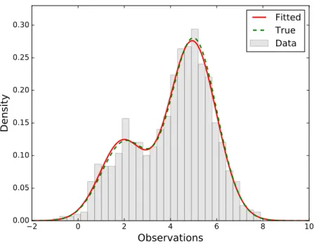
To illustrate the process of parameter estimation for a FMM via the EM algorithm, we implemented a fitting process, with threshold = 0.000001, to a two-component Normal mixture model with weightsπ1=0.3 andπ2=0.7, equal variancesσ₁2=σ₂2=1 and different means, µ1=2 and µ2=5. Both Table (2.1) and Figure (2.2) show results of the estimation process

using the EM procedure.

Parameter π1 µ1 µ2 σ12 σ22

True 0.3 2 5 1 1

Estimated 0.291 1.928 4.948 0.902 1.012

Table 2.1:The true and estimated values of a two-component Normal mixture model using EM algorithm for a simulated sample of 1000 observations.

2 0 2 4 6 8 10

Observations

0.00 0.05 0.10 0.15 0.20 0.25 0.30

Density

Fitted

True

Data

Figure 2.2:Fitting a two-component Normal mixture model using the EM algorithm.

2.3.2 The Bayesian estimation of FMMs

In the FMM in Equation (2.1), the unknown parameter vector Θ= (π;θθ) needs to be estimated. In order to obtain the posterior distribution of Θ, we need to combine the data-dependent likelihood functionL(Θ;y) of the mixture model and the prior distribution of the unknown parametersΘ= (π;θθ). By assuming the independence of the prior distributions of the model parameters;θθandπ, the posterior distributionPr(Θ|y)can be given as

Model Fit Diagnostics for Hidden Markov Models

by

Safaa K. Kadhem

A thesis submitted to Plymouth University in partial fulfillment of the

requirements for the degree of

DOCTOR OF PHILOSOPHY

School of Computing, Electronics and Mathematics

Faculty of Science and Engineering

Plymouth University

Abstract

Contents

List of Figures

List of Tables

Introduction

∏

∏

∑

∏

∑

∑

∑

∑

∑

∑

∑

Finite Mixture Models

∑

∑

∑

∑

(a)

(b)

(c)

(d)

0.40

0.35

0.30

0.25

0.20

0.15

0.10

0.05

0.00 6 4 2 0 2 4 6 8

0.25

0.20

0.15

0.10

0.05

0.00 6 4 2 0 2 4 6 8

0.00 6 4 2 0 2 4 6 8

0.20

0.15

0.10

0.05

0.20

0.15

0.10

0.05

0.00 6 4 2 0 2 4 6 8

∏

∏

∑

∏

∏

∏

∏

∑

∑

∑

∑

∑

∑

∑

∑

∑

∑

∑

∑

∑

∑

_∑

_∑