6
Traditional Demand Theory
We have already discussed some examples of comparative statics in pervious lectures and homework exercises. However, we have spent a big share of our energy discussing how to formulate and solve problems of rational choice in di¤erent versions. Now, we will switch the focus somewhat and try to be more systematic in our approach to comparative statics. In general, comparative statics is an exercise where we analyze how the behavior changes when di¤erent variables in the environment changes. That is, we try to predict what the behavioral response to di¤erent (to the consumer) exogenous changes should be. This sort of an exercise is what a large share of economics is about, and we will do it in many other applications in the rest of the class. For now, however, we will study what happens as prices and income changes for the consumer ,which is the topic of traditional demand theory (one of the oldest and most well developed branches of economic theory).
6 -6 -x1 x2 x2 x1 Z Z Z Z Z Z Z Z Z Z Z Z Z Z ZZ e e e e e e e e e e e e x1 x2 Z Z Z Z Z Z Z Z Z Z Z Z Z Z ZZ x1 x2 Z Z Z Z Z Z Z Z Z Z Z Z Z Z Z Z Z Z ZZ
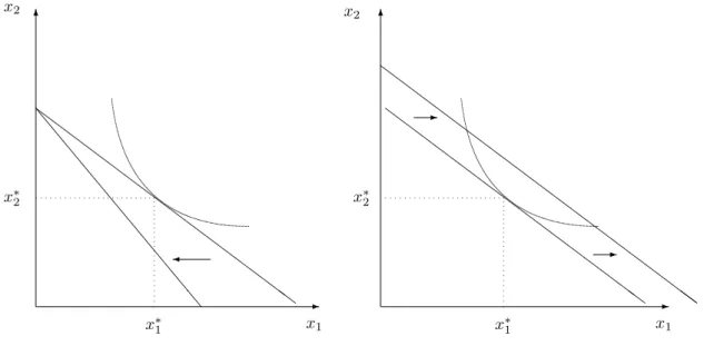
-Figure 1: A Change in Price or Income Changes the Solution
The …rst fact to realize is trivial, but important: the optimal consumer choice depends on p1; p2 and m:This should be obvious from a graph. In Figure 1 I’ve indicated an optimal
solution given some initial prices and income (x1; x2). In the left graph we see that when the price increases, then the old optimal bundle is no longer a¤ordable, so the optimal solution
with a higher price on good one must be some di¤erent bundle (somewhere along new budget line). To the right we see that when income increases there are now bundles better than the old optimal solution that are a¤ordable, so the solution must change here as well.
Since we now will start to vary p1; p2 andm we want notation that makes this clear. We
write
x1(p1; p2; m)
x2(p1; p2; m)
for thedemand functions associated with some particular utility function. What this means in terms of our optimization problem is thatx1(p1; p2; m)and x2(p1; p2; m)together
consti-tute an optimal solution to
max x1;x2
u(x1; x2)
s.t p1x1+p2x2 m
Example 1 Cobb-Douglas. We have actually already solved for the demand functions in class. x1(p1; p2; m) and x2(p1; p2; m) solves
maxxa1x12 a
s.t p1x1+p2x2 m
and we already know that
x1(p1; p2; m) = am p1 x2(p1; p2; m) = (1 a)m p2
Special property of Cobb-Douglas: demand for good 1independent of price of good 2and vice versa. This is not true in general. Also note that the parameter from the utility function
a enters the formula for the demand generated by Cobb-Douglas preferences. Still, we don’t think of the demand function as a function of a: The reason is that a is a deep
parame-ter re‡ecting the preferences and comparisons of di¤erent as would be to compare di¤erent
6.1
Changes in Income
6 -6 -x1 x2 x1 m e e e e e ee @ @ @ @ @ @ @ @ @ @@ @ @ @ @ @ @ @ @ @ @ @ @ @ @ m0 p1 m00 p1 m000 p1 m0 m00 m000 x0 1 x001x0001 x01 x001 x0001 u u u Engel Curve u u uIncome O¤er Curve
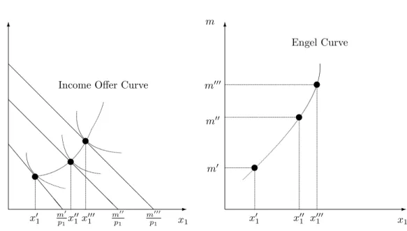
Figure 2: Graphical Derivation of Engel Curve
Now, the demand function takes on a quantity for each triple(p1; p2; m)so to graph these
things we have to project down into lower dimensions. One of the obvious experiments to do is then to …x prices and see how the solution changes as income changes but prices are …x. This projection of the demand function is called anEngel curve and the graphical derivation of an Engel curve is shown in Figure 2. Observe that while the natural convention would be to plot x1 on the vertical axis and m on the horizontal, the opposite convention was
established some time in the dark ages and economists got stuck with this.
Notice that whether the consumer increases or decreases the consumption of a particular good when the income increases depends on the preferences. That is, in the Cobb Douglas example we directly see thatx1(p1; p2; m) = amp1 andx2(p1; p2; m) =
(1 a)m
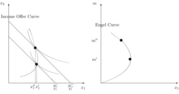
p2 are both increas-ing in m: In contrast, Figure 3, which is drawn with preferences that satisfy monotonicity and convexity, shows an example where the consumption if x1 is decreasing in m over an
interval (observe, since consumption is zero whenm = 0 it must be that the consumption is initially increasing inm to make it possible for the curve to bend backwards)
6 -6 -x1 x2 x1 m @ @ @ @ @ @ @ @ @ @@ @ @ @ @ @ @ @ @ @ @ @ @ @ @ m0 p1 m00 p1 u u m0 m00 u u x0 1 x00 1
Income O¤er Curve
Engel Curve
Figure 3: An Inferior Good
The conclusion is thus that we cannot a priori say anything about whether the consump-tion is increasing or decreasing in income. For future reference we will simply create some terminology that assigns names to the di¤erent cases:
De…nition 2 Good 1(2) is said to be a normal good if x1(p1; p2; m) (x2(p1; p2; m)) is
in-creasing in m
De…nition 3 Good 1(2) is said to be an inferior good if x1(p1; p2; m) (x2(p1; p2; m)) is
decreasing in m
In concrete examples one can either just look at the demand function to see if it is increasing in m or not. If the demand function is more complicated, t is sometimes useful to observe that one can check this by looking at the partial derivative
@x1(p1; p2; m)
@m :
In the Cobb-Douglas case@x1(p1;p2;m)
@m =
a
p1 >0:In general, normality corresponds to a positive partial derivative with respect to income, and inferiority corresponds with a negative partial derivative.
Typically normality is taken to mean that the quantity demanded is increasing in m
for all (p1; p2); but conventions di¤er and I will not be picky on things like that. Observe
however that it is impossible for a good to be “always inferior”. If one wants to be careful, one also has to make ones mind up whether @x1(p1;p2;m)
@m 0or
@x1(p1;p2;m)
@m >0is the criterion
for normality, but you need not worry too much about that detail.
6.2
Changes in Prices
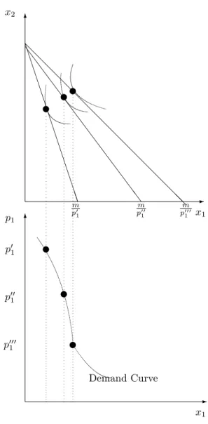
The next obvious experiment is to see how a demand function behaves as m and the price of the other good(s) are held constant. This projection of the demand function is called the demand curve. Figure 4 shows how this curve can in principle be derived from the usual indi¤erence curve graph. Notice the convention (which has stuck for historical reasons) that (the “independent variable”) price is on the vertical axis.
Maybe more surprisingly (unless you’ve seen it in an earlier class) the e¤ect on consump-tion from a change in the price is also ambiguous. If we again look at the Cobb-Douglas example we see that
@x1(p1; p2; m) @p1 = am p2 1 <0 @x2(p1; p2; m) @p2 = (1 a)m p2 2 <0;
so in this case the e¤ect from a price increase is what one would intuitively expect-a decrease. However, it is possible that consumption of a good decreases when the price decreases, which graphically corresponds to an upwards sloping demand curve. Notice (we will come back to this) that the indi¤erence curves in the graphical construction of an upward sloping demand in Figure 5 look remarkably similar to those of an inferior good.
The conventional terminology (which isn’t used as much as the normal/inferior distinction for reasons that will become apparent) is:
De…nition 4 Good 1(2) is said to be a ordinary good if x1(p1; p2; m) (x2(p1; p2; m)) is
6 -6 -x2 x1 p1 x1 B B B B B B B B B B B B B B BB S S S S S S S S S S S S S S S @ @ @ @ @ @ @ @ @ @ @ @ @ @ @@ m p0 1 m p00 1 m p000 1 p0 1 p00 1 p000 1 u u u u u u Demand Curve
Figure 4: Graphical Derivation of (Inverse) Demand Curve-Ordninary Good
De…nition 5 Good 1(2) is said to be a Gi¤en good if x1(p1; p2; m) (x2(p1; p2; m)) is
de-creasing in p1 (p2)
Again, sometimes the easiest way to check is by taking the partial derivative with respect to (own) price.
6 -6 -x2 x1 p1 x1 B B B B B B B B B B B B B B BB S S S S S S S S S S S S S S S @ @ @ @ @ @ @ @ @ @ @ @ @ @ @@ m p0 1 m p00 1 m p000 1 p0 1 p00 1 p000 1 u u u u u u Demand Curve
Figure 5: A Gi¤en Good
6.3
Examples
6.3.1 Cobb Douglas Preferences We have that
x1(p1; p2; m) =
am p1
and to draw an Engel curve we only need to set a; p1 to some speci…c values and plot the
relation between m and x1:Say for concreteness that a= 1=2 and p1 = 4)
x1(4; p2; m) = 1 2 m 4 = m 8 ) m= 8x1;
so the Engel curve is a straight line starting at the origin with slope8
6
-x1
m
Figure 6: The Engel Curve foru(x1; x2) =x
1 2
1x
1 2
2 …ven any p2 and p1 = 4
In general we see that
x1 = am p1 x2 = (1 a)m p2
Since the relationship between x1 and m is linear we see from this that the Engel curves
are straight (upwards sloping) lines starting at the origin. Hence, good 1 is a normal good and everything is symmetric for good 2 so we conclude that both goods are normal for a consumer with Cobb Douglas preferences
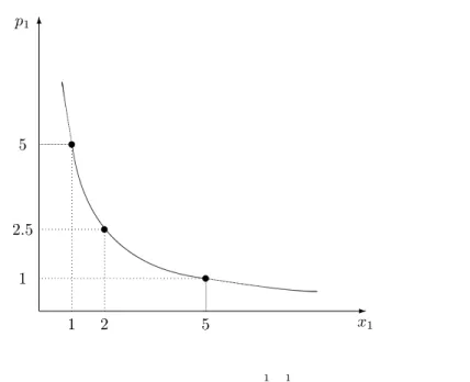
To sketch the demand curve for good 1 we …x a and m and vary p1: If we again set the
preference parametera= 1=2and set m= 10 we get
x1 = 1 10
2p1 ,
p1 = 5x1;
6 -x1 p1 s s s 5 2:5 1 1 2 5
Figure 7: The Demand Curve for u(x1; x2) = x
1 2
1x
1 2
2 …ven any p2 and m = 10
Again we see that in general, the (inverse) demand curves are given by
p1 = am x1 p2 = (1 a)m x2 ;
where you should think ofmas a constant when you plot these curves. Obviously this means that demand curves are downward sloping, so we conclude that both goods are ordinary
6.3.2 Perfect Substitutes
u(x1; x2) = 5x1+x2:
Recall from one of your homework exercises that this utility function generates interior solutions only in knife-edge cases. Indi¤erence curves are straight lines, so the typical case is a corner solution (draw picture if you don’t see this!). The only tricky part is to determine when (that is for which prices & income) which corner is optimal and the easy way to this is to check what happens if the consumer spends everything on x1; that is (x1; x2) = pm
1;0 : The corresponding value of the utility function is
5m
p1
If on the other hand the consumer spends everything onx2; then the utility is
m p2
:
Clearly, spending everything on x1 (x2) is better if 5pm1 > pm2 , pp21 <5 (5pm1 < pm2 , pp12 > 5),
while the consumer is indi¤erent if p1
p2 = 5: Thus the demand curve is
x1(p1; p2; m) = 8 > > > > < > > > > : m p1 if p1 p2 <5 h 0;pm 1 i if p1 p2 = 5 0 if p1 p2 >5 :
As an example, considerp1 =p2 = 1)slope of budget line: 1 )Engel curve for good 1: m =x1
)Engel curve for good 2: x2 = 0 for all m (follows vertical axis)
Given that we only require the demand to be weakly increasing in income, this is consis-tent with normality.
Demand curve: Set m = 10; p2 = 1
6 -x1 p1 5 2 5
Figure 8: Demand Curve foru(x1; x2) = 5x1+x2 given m= 10 and p2 = 2
x1 = 0 forp1 >5
[0;2]for p1 = 5
decreasing over p1 in[0;5]
If we allow ordinary goods to have ranges where the demand is constant, this is an ordinary good.
6.4
Substitutes and Complements
Final question-how is the demand of x1 a¤ected by a change in p2: Know that for perfect
complements the demand is decreasing since
ax1(p1; p2; m) = bx2(p1; p2; m)
The demand can then by found by solving
p1x1(p1; p2; m) +p2 a bx1(p1; p2; m) = m) x1(p1; p2; m) = m p1 +p2ab
so x1 & when p2 %: On the other hand, for perfect substitutes, either nothing happens or
an increase inp2 )x1 %: Given these examples the following de…nitions seem natural:
6.4.1 (Gross) Substitutes If x1(p1; p2; m) is increasing in p2
6.4.2 (Gross) Complements If x1(p1; p2; m) is deceasing inp2
You can check that goods are neither substitutes or complements for Cobb-Douglas, substitutes for perfect substitutes and complements for perfect complements.
6.5
Income & Substitution E¤ects
This is covered in Varian Chapter 8 (8.1-8.5 and 8.7).We found from straightforward indi¤erence curve analysis that (in the case of a Gi¤en good) it is indeed possible that the demand is increasing in price. While we think that this is primarily a curiosity (that is, the conventional wisdom is that most goods are not like this) it is instructive to think about why this can happen.
Brie‡y put, the answer is that two things happen when the price of a good goes down. First of all the relative price changes making the good cheaper in terms of other good.
Moreover, the purchasing power of the consumer increasesa fall in one price makes the consumer richer since consumption of all goods can now be increased.
We will now try to separate out these e¤ects into income and substitution e¤ects. You should be warned that there are two di¤erent ways to do this. Exactly as in Varian I will spend most time explaining the diagrammatically most straightforward decomposition (called the Slutsky decomposition), but check Varian 8.8 for another possible decomposition.
6 -A A A A A A A A A A A A A A A AA l l l l l l l l l l l l l l l l l l ll m p1 m p0 1 s l l l l l l l l l l l l l l ll s s x1 x2 p01x1+p2x2 p0 1 x x0 x00 S u b s t E ¤e c t In c o m e E ¤e c t
-Figure 9: Substitution and Income E¤ects
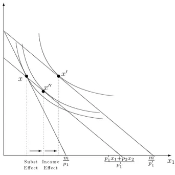
The idea is that we can “control”for the fact that the consumer gets richer when the price falls by adjusting the income so that the old optimal bundle is on the budget line with the new relative prices. The optimal bundle for this …ctitious budget set is what the consumer would optimally choose under the new prices if income was taken away so as to make the old optimal bundle barely a¤ordable. Hence the di¤erence between this and the old consumption can be thought of as the change in consumption that is attributed to the change in relative prices and this change is what is called the SUBSTITUTION EFFECT.
The INCOME EFFECT is then the change from this (hypothetical) bundle with new relative prices and adjusted income to the optimal bundle with the new prices and the (unchanged) income that the consumer actually has.
This is illustrated in Figure 9 where x= (x1; x2) is the demand given(p1; p2; m)and x0 is
the demand given (p0
1; p2; m)(the only change is the price of good 1 that has decreased from
p1 top01). Diagrammatically, thesubstitution e¤ect is found by “pivoting”the budget line so
that a new budget line with slope p01
p2 that goes though the old optimal bundle is constructed. The substitution e¤ect is then the di¤erence between the demand given this new budget line and the original demand. The income e¤ect is the di¤erence between the demand given the price change (the “real thing”with unchanged income) and the (hypothetical) demand just constructed (x00 in the picture)
To explain this somewhat more carefully it is useful to use the notation for demand functions we’ve introduced
1. The income that keeps (x1(p1; p2; m); x2(p1; p2; m)) exactly on the budget line when
the price of good 1 changes fromp1 top01 is
m0 =p01x1(p1; p2; m) +p2x2(p1; p2; m)
2. The TOTAL EFFECT on the demand of good 1 the price of good 1 changes from
p1 top01 is
x1 =x1(p01; p2; m) x1(p1; p2; m)
3. The SUBSTITUTION EFFECT is
xS1 =x1(p01; p2; m0) x1(p1; p2; m)
4. The INCOME EFFECT is
xN1 =x1(p01; p2; m) x1(p01; p2; m0)
In words:
2. Substitution e¤ect: e¤ect on demand from a price change from p1 top01 and a
simulta-neous income change fromm tom0 where m0 is calculated as to make the old demand
exactly a¤ordable at new prices
3. Income e¤ect: e¤ect on demand from a change in income from m0 to m: (given new prices).
Observe …nally that the decomposition is OK since
xS1 + xN1 = x1(p01; p2; m0) x1(p1; p2; m) +x1(p01; p2; m) x1(p01; p2; m0)
= x1(p01; p2; m) x1(p1; p2; m) = x1
6.6
Example:
Computing Substitution and Income E¤ects for
Cobb-Douglas Preferences
Recall that if u(x1; x2) =xa1x 1 a
2 ; the demand functions are
x1(p1; p2; m) = am p1 x2(p1; p2; m) = (1 a)m p2 :
For concreteness, set a= 12 and let(p1; p2; m) = (2;2;40): Consider a change in the price of
good 1 fromp1 = 2 to p01 = 1) x1(2;2;40) = 1 2 40 2 = 10 x2(2;2;40) = 1 2 40 2 = 10 x1(1;2;40) = 1 2 40 1 = 20
)The total e¤ect is given by
To compute the substitution e¤ect we solve for
m0 = 1 x1(2;2;40) + 2x2(2;2;40) =
= 1 10 + 2 10 = 30;
so the substitution e¤ect is
xS1 =x1(1;2;30) x1(2;2;40) =
1 2
30
1 10 = 15 10 = 5:
The income e¤ect is
xN1 =x1(1;2;40) x1(1;2;30) = 20 15 = 5;
but really we already knew this since in general
xN1 = x1 xS1
and we had already computed x1 = 10 and xS1 = 5:
6.7
Sign of the Substitution E¤ect
Clearly, the income e¤ect may be negative or positive depending on whether the good is normal or not, but the substitution e¤ect can be signed, which is why the decomposition is of some use in economics.
Claim The substitution e¤ect is always negative.
What this means is that when p1 goes up (and income is adjusted), the demand goes
down, while if p1 goes down, then the demand goes down after the adjustment in income.
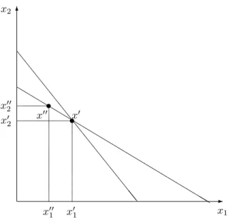
To see this look at Figure 10, where x0 = (x0
1; x02) is the optimal bundle given some prices
and income (corresponding with the steeper budget line). Now, if the substitution e¤ect tends to decrease the consumption when the price on good one goes down, the new optimal bundle must be to the left of x0 on the pivoted budget line. Call this bundle x00: Now, the
6 -\ \ \ \ \ \ \ \ \ \ \ \ \ \\ bb bb bb bb bb bb bb bb bb b s s x0 x00 x1 x0 1 x00 1 x0 2 x00 2 x2
Figure 10: Why Substitution E¤ect can’t be Positive
the consumer could have bought x00 before. Moreover, if preferences are monotonic, then everything to the northeast of x00 is strictly better than x00 which must be at least as good
asx0 was a¤ordable giventhe old prices and income. Hence,x0 could not have been optimal
in the …rst place. The conclusion of this is that the optimal bundle after the pivot must be somewhere to the right of x0 on the pivoted budget line, so the demand increases when the
price goes down. The exact same argument works for a price increase as well.
Remark: The argument uses the principle ofrevealed preference. We will not spend too much time on this in this class, but you should know that this principle makes it possible to “observe preferences”. Indeed, since we could get data thatviolates revealed preference, this makes our model of rational choice refutable, meaning that this is actually something that quali…es as a scienti…c theory. See chapter 7 in Varian …r details on how revealed preference can be used to draw inference about preferences.
WE CAN THEN CONCLUDE:
1. p01 < p1 )x1(p01; p2; m0) x1(p1; p2; m)
2. p0
where
m0 =p01x1(p1; p2; m) +p2x2(p1; p2; m)
6.8
Sign of the Income E¤ect
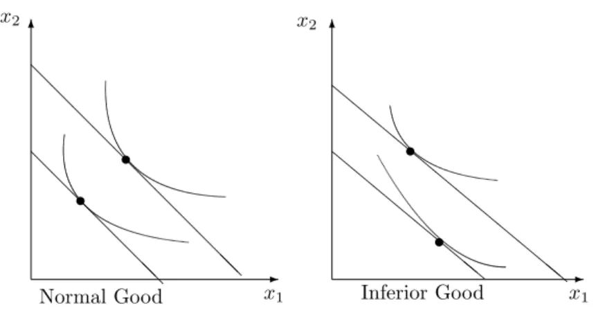
6 -6 -x1 x2 x2 x1 @ @ @ @ @ @@ @ @ @ @ @ @ @ @ @ @@ l l l l l l ll l l l l l l l l l l ll s s s sNormal Good Inferior Good
Figure 11: Income E¤ect for Normal vs Inferior Good
The income e¤ect clearly depends on whether the good is normal or inferior and the only thing to watch out for is the direction of the shifts. First of all note that if x = (x1; x2) is
the demanded bundle given(p1; p2; m); then
m0 = p01x1+p2x2 (de…nition of pivot)
m = p1x1+p2x2 (since x is optimal)on budget line)
Combining these we have
m=m0 m =x1(p01 p1) =x1 p1;
so p1 >0, m >0: SAME SIGN, so
Increased price )Increased Income Decreased price)Decreased Income, so we say that
The income e¤ect is negative for normal goods (sincep1 %)m% and the “e¤ect”is
The income e¤ect ispositive for inferior goods.
6.9
A Gi¤en Good is “Very Inferior”
The easy way to think about these things is to imagine an increase in price. However, interpreting “ ” as “opposite of the sign of the change in the price” and “+” as the same sign as the change in the price the expressions below are true no matter which way the price changes.
CASE 1: If good 1 is anormal good, everything is clear since
x1 negative = x S 1 negative (always) + x N 1
negative (def of normal good)
)Normal goods have downward sloping demand curves. CASE 2: If good 1 is inferior, then
x1 ? = xS1 negative (always) + x N 1
Positive (def of inferior good)
Hence, if the income e¤ect is strong enough it may dominate the substitution e¤ect) x1
may be positive (meaning that it moves in the same direction as the change in the price), in which case good 1 is a Gi¤en good. The conclusion of this is that any Gi¤en good must be an inferior good (while the opposite implication doesn’t hold), so it is no coincidence that examples for inferior and Gi¤en good often coincide.
I am not an empirical economist, but, according to colleagues, there is no convincing empirical study that has been able to …nd a real-world Gi¤en good. I don’t think that is too surprising. The income e¤ects need to be large for the income e¤ects to dominate the substitution e¤ects, and for that to be the case the good in question must be a fairly important good in the sense that a quite large share of the income is spent on it. Typical textbook examples of Gi¤en goods are potatoes on Ireland or rice in China (this is also the kind of goods empricists have looked at in vain), but it seems doubtful that the consumption of the basic source of carbohydrates would decline as income rises. Rather, one would expect
people to eat as much potatoes (or more) as before and top it up with some meat, vegetables, and maybe a Guiness or two
7
Labor Supply
Varian pages 171-176 (but ignore his terminology about “endowment income e¤ects”. Before starting with equilibrium theory I will discuss one …nal application/interpretation of the standard consumer choice model that I have postponed because I wanted to talk about income and substitution e¤ects before discussing it.
We now think about an agent who likes consumption, dislikes work (who doesn’t rather spend time watching “Who wants to...”) and is selling his/her time on the market. Let
C be consumption
p be the price of the consumption good
L be the amount of labor supplied
L be the endowment of time (i.e., 24 hours)
w be the wage (dollars per unit of time)
M be non-labor income
The sceptic may …nd it strange that although supply of labor has an obvious time dimen-sion, consumption has not. This is a fair complaint, but as usual we are abstracting away from lots of realism in order to make the model as simple as possible. Still, this basic model has proven to be very useful and is still used in labor economics extensively.
7.1
The Budget Constraint
The obvious way to write down the budget constraint is to observe that Expenditures=total income, that is
This form is …ne for setting up the relevant maximization problem, but not very useful for drawing indi¤erence curve graphs. Instead, we observe that
pC = M +wL:,
pC wL = M , add wL on both sides
:pC+w L L = M +wL
Finally let C be the consumption the consumer would have if not working, that is
C = M
p
and we can write the budget constraint as
pC +w L L | {z } leisure = pC +wL | {z } value of endowment
This form of the budget constraint should make clear that we can think of the labor sup-ply problem in the same way as the standard model, where the consumer is purchasing consumption goods and leisure.6
-l l l l l l l l l l l llr C L L L C Slope w p
Figure 12: The Budget Set for the Labor Supply Problem
The way to think about it is that if the consumer doesn’t trade then he/she consumes the endowment, which isC units of the consumption good andL units of leisure. However,
the consumer can trade leisure for consumption by supplying labor in the market. Note here that:
1. wis the price, or opportunity cost, of leisure. The point of this is that if you think that it is free to watch The Bachelor (or The Bachelorette) you should seriously rethink! What you pay for doing it is the income you would earn if you went out working the time spent on the couch (or, in a richer model where you can invest in future earnings opportunities by getting a good grade in Econ 301, your present value of the expected extra earning you would get by spending that extra time on your homework problem for Friday).
2. The slope of the budget line, w=p is usually referred to as the real wage.
7.2
Optimal Labor Supply Decisions
We now assume that the consumer has some preferences over consumption and leisure given by
U C; L L
Substituting in the budget constraint gives the problem in the usual form
max 0 L L
U C+w
pL; L L
and the …rst order condition will give a tangency condition of exactly the same form as before with the interpretation that the marginal rate of substitution between consumption and leisure has to be equalized with the slope of the budget constraint. The optimal labor supply decision is depicted in Figure 13.
You should all try to …nd the relevant …rst order conditions and think about them, I will restrict myself to graphical analysis.
Question: Suppose the wage goes up, what happens with labor supply?
Seems to be a relevant question. Often argued that reducing taxation on income will lead to more incentives to supply labor) more goods produced....
6 -l l l l l l l l l l l llr C L L L C Slope wp r -Leisure -Labor
Figure 13: Optimal Labor Supply
For simplicity let M = 0 (no non-labor income). To graph the budget set we then note that the intercept at the leisure axis in L; while if the consumer has no leisure the (dollar) income is wL; so that the intercept with the consumption axis is that wLp : Figure 14 shows the e¤ect of increasing the wage from w tow0 and we note that:
An increase in the wage is exactly as a decrease in price of the consumption good.
Hence, how consumption of leisure (supply of labor) is a¤ected depends on whether leisure and the consumption good aresubstitutes orcomplements. You are encouraged to work out details!
An alternative way to look at it is to decompose the change in income and substitution e¤ects:
Substitution E¤ect w=p%)leisure more expensive)work more/less leisure.
Income E¤ect w=p %)consumer richer and can increase consumption of both goods. If leisure is a NORMAL good) consumer “buys” more leisure.
6 -C H H H H H H H H H H H H H @ @ @ @ @ @ @ @ @ @ @ @ @ wL p w0L p L L L
Figure 14: E¤ect on Budget Set From Higher Wage
THUS: INCOME AND SUBSTITUTION EFFECTS TEND TO GO IN OPPOSITE DIRECTIONS FORNORMALGOODS RATHER THAN FOR INFERIOR GOODS (AS IN STANDARD TWO GOODS MODEL).
Since there seem to be no a priori reason why leisure should be inferior we expect small responses in terms of labor supply and even backwards bending at high incomes. Eventually this means that the response to changes in the real wage is an empirical question and while the evidence is mixed small responses is the norm and backwards bending has been found in lots of studies.
7.3
Example: Cobb-Douglas Preferences
I assume no non-labor income. The problem is then to solvemax C;L lnC+ (1 ) ln L L subj to pC = wL or max 0 L L ln w pL + (1 ) ln L L
6 -l l l l l l l l l l l llr C L L L C Slope wp r T T T T T T T T T T T T T T J J J J J J J J J J J J J J J J J J J r r
-Figure 15: Substitution and Income E¤ects (Income E¤ect Dominating)
FOC w pL w p + (1 ) L L ( 1) = 0, L L = (1 )L L w p = L
Labor supply constant function of real wage.