Control Design and Implementation of an Active Transtibial Prosthesis

Master's Theses (2009 -) Dissertations, Theses, and Professional Projects

Control Design and Implementation of an Active

Transtibial Prosthesis

Joseph Klein

Recommended Citation

Klein, Joseph, "Control Design and Implementation of an Active Transtibial Prosthesis" (2018).Master's Theses (2009 -). 481. https://epublications.marquette.edu/theses_open/481

by

Joseph G. Klein, B.S.

A Thesis Submitted to the Faculty of the Graduate School, Marquette University, in Partial Fulfillment of the Requirements for

the Degree of Master of Science

Milwaukee, Wisconsin August 2018

PROSTHESIS

Joseph G. Klein, B.S. Marquette University, 2018

Prior work at Marquette University developed the Marquette Prosthesis, an active transtibial prosthesis that utilized a torsional spring and a four-bar

mechanism. The controls for the Marquette Prosthesis implemented a finite state control algorithm to determine the state of gait of the amputee along with two lower level controllers, a PI moment controller to control the moment during stance and a PID position controller to control the position during stance. The Marquette

Prosthesis was successful in mimicking the gait profile presented by Winter. However, after completing human subject testing, the Marquette Prosthesis was insufficient in trying to match the gait profile of those who varied from this textbook stride.

Active transtibial prostheses typically apply finite state control algorithms that struggle with cadence and gait variability of the amputee. Recent work in artificial neural networks (ANN) have shown the possibility to predict the user’s intent which can be used as an input signal in an improved controller. The

Marquette Prosthesis II was developed that uses a stiffness controller to control the relationship between the position and torque of the ankle. A model of the improved Marquette Prosthesis II was developed in Simulink to ensure that the stiffness controller was robust enough and that this type of control was possible with the limitations of the Marquette Prosthesis, i.e., the link lengths, torsional spring and motor. The mechanical system of the Marquette Prosthesis was then changed such that the spring was in series between the motor and four-bar mechanism to establish a relationship between the motor position, torque of the spring and four-bar

mechanism. The control hardware was selected and the stiffness controller was implemented on the Marquette Prosthesis II. The Marquette Prosthesis II control algorithm was tested and validated to show that this approach is feasible.

ACKNOWLEDGMENTS

Joseph G. Klein, B.S.

I would like to thank my Mom, Dad and siblings for their continued support and inspiration. I would like to thank Dr. Philip Voglewede for being an incredible advisor and mentor to me over the past two years, pushing me to be a better person and engineer. I would like to thank Tony Buchta, Ryan Callahan, Jack Alberts and Shaoli Wu for the countless conversations and support in the Wede lab. I would like to thank my friends for helping me to keep my sanity over the past two years and being as excited as I am about the success of this project. I would like to thank Erika Zabre for her patience and help in running the tests with me in the Human Performance Laboratory. I would like to thank Dr. Mark Nagurka for his passion for engineering and pushing me to be a better engineer. I would like to thank Dr. Aderiano daSilva for pushing me to pursue a career in controls and teaching me how to be a better controls engineer. Finally, I would like to thank Marquette University and all of those at Marquette who have helped me develop into the person and engineer I am.

TABLE OF CONTENTS

ACKNOWLEDGMENTS . . . i

LIST OF TABLES . . . vi

LIST OF FIGURES . . . vii

CHAPTER 1 Introduction . . . 1

1.1 Motivation . . . 1

1.2 Fundamental Causes of Transtibial Amputation . . . 1

1.3 Development of Lower Limb Prostheses . . . 3

1.3.1 Passive Prostheses . . . 4

1.3.2 Active Prostheses . . . 4

1.4 Development of Artificial Neural Network . . . 5

1.5 Motivation for this Research . . . 6

1.6 Scope . . . 7

1.7 Research Contributions . . . 8

CHAPTER 2 Literature Review . . . 10

2.1 Myoelectric Control of Powered Upper Limb Prostheses . . . 10

2.1.1 Weighting Synergistic Muscle Movements - Temple University 12 2.1.2 Endpoint Control - University of California, Los Angeles . . . 14

2.1.3 Transient Myoelectric Control - University of New

Brunswick in Canada . . . 15

2.2 Mechanical and Control Systems of Lower Limb Prostheses . . . 17

2.2.1 Ossur Propio Foot with Evo . . . .¨ 19

2.2.2 BioM - MIT Powered Ankle-Foot Prosthesis . . . 19

2.2.3 SPARKy 3 - ASU Powered Ankle-Foot Prosthesis . . . 25

2.2.4 Vanderbilt University Powered Ankle and Knee Prosthesis . . 31

2.2.5 System Hardware . . . 34

2.3 Summary . . . 35

2.4 Marquette Prosthesis . . . 35

CHAPTER 3 Dynamic Model and Simulation . . . 37

3.1 Four Bar Mechanism Analysis . . . 38

3.1.1 Kinematics . . . 39

3.1.2 Quasi-statics . . . 42

3.2 Simulink Model . . . 43

3.2.1 Dynamic Simulation and PI Tuning . . . 44

3.2.2 Investigation of Linear Spiral Spring . . . 46

3.2.3 Effect of Spring Constant on Output Torque . . . 47

3.2.4 Motor Torque and Speed Capabilities . . . 49

CHAPTER 4 Mechanical System Redesign . . . 51

4.1 Redesign of Link 3 to move spring in Series . . . 53

4.1.1 Press Fit Analysis . . . 56

CHAPTER 5 Control System Architecture and Implementation . . 58

5.1 Overall Control System Architecture . . . 58

5.2 Controller Implementation . . . 59

5.2.1 Computer System Overview of Other Successful Prostheses . . 60

5.2.2 Selection of Control Hardware for Marquette Prosthesis II . . 64

5.2.3 Selection of Sensor Hardware for Marquette Prosthesis II . . . 65

5.2.4 Marquette Prosthesis II Hardware compared to Marquette Prosthesis Hardware . . . 66

CHAPTER 6 Bench Testing . . . 71

6.1 Stiffness Control Testing . . . 71

6.2 Bench Testing . . . 72

6.2.1 Hanging Hand Test Procedure . . . 72

6.2.2 Hanging Hand Test Results . . . 74

6.2.3 Force Hand Test Procedure . . . 76

6.2.4 Force Hand Test Results . . . 79

CHAPTER 7 Conclusion and Future Work . . . 88

7.2 Future Work . . . 91

7.2.1 Implementation of ANN . . . 92

7.2.2 Redesign of the Four-Bar Mechanism . . . 92

7.2.3 Reselection of Linear Spiral Torsional Spring . . . 93

7.2.4 Reselection of Motor . . . 94

7.2.5 Higher Level Controller . . . 95

References . . . 96

APPENDIX A Four Bar Kinematics . . . 101

APPENDIX B Four Bar Quasi-statics . . . 105

APPENDIX C Simulink Model . . . 110

APPENDIX D Control Block Diagram . . . 116

APPENDIX E Calculating Ankle Moment from Force Plate and Kine-matic Data . . . 119

LIST OF TABLES

3.1 Final Parameters for Tuned Controller . . . 46

5.1 Mass of Components for Marquette Prosthesis . . . 68

5.2 Mass of Components for Marquette Prosthesis II . . . 68

5.3 Size of Components for Marquette Prosthesis . . . 70

LIST OF FIGURES

2.1 Block Diagram of Myoelectric Controlled Prosthesis [13] . . . 11

2.2 Block Diagram of UNB Control System [13] . . . 17

2.3 Schematic of the BioM Ankle-Foot Prosthesis [4] . . . 20

2.4 BioM Controller Architecture [4] . . . 22

2.5 Computer System of BioM [4] . . . 25

2.6 Robotic Tendon Model: Motor and Spring in Series [23] . . . 27

2.7 Two Degrees-of-Freedom SPARKy Model [21] . . . 27

2.8 CAD Model of SPARKy 3 [22] . . . 28

2.9 Tibia Angle Profile vs Human Gait. Each curve represents a different stride length [22] . . . 29

2.10 SPARKy 3 Control Hardware [22] . . . 30

2.11 Slider Crank Configuration [41] . . . 32

2.12 Knee and Ankle Prosthesis with Major Components [41] . . . 32

2.13 Powered Ankle and Knee Prosthesis Control Structure [43] . . . 33

2.14 Embedded System Framework [41] . . . 34

3.1 Model of the Marquette Prosthesis II . . . 39

3.2 Sketch of the Four-Bar Mechanism . . . 40

3.4 Desired Ankle Angle versus Actual Ankle Angle . . . 46

3.5 Desired Ankle Torque versus Actual Ankle Torque with Original Spring . 47 3.6 Effect of Spring Constant on Motor Torque . . . 48

3.7 Required Speed Torque of Motor Compared to Motor Speed Torque Curve 49 4.1 Model of Marquette Prosthesis with Spring in Parallel with the Motor Adopted from [40] . . . 52

4.2 Model of Marquette Prosthesis II with Spring in Series with the Motor . 52 4.3 Mount that Connects the Spiral Torsion Spring to Link 0 . . . 53

4.4 Redesign of Link 3 . . . 54

4.5 Linear Spiral Torsional Spring . . . 55

4.6 Side View of Assembly of Link 3 and Linear Spiral Torsional Spring . . . 55

4.7 ANSYS Deformation Results . . . 57

4.8 ANSYS Stress Results . . . 57

5.1 Block Diagram Representation of Control System . . . 59

5.2 Massachusetts Institute of Technology Hardware Flow . . . 62

5.3 Arizona State University Hardware Flow . . . 62

5.4 Vanderbilt University Hardware Flow . . . 63

5.5 Marquette Prosthesis Hardware Flow . . . 63

5.6 Marquette Prosthesis II Hardware Flow . . . 66

6.2 Side View of Marquette Prosthesis II with Hardware Attached . . . 73

6.3 Back View of Marquette Prosthesis II with Hardware Attached . . . 74

6.4 Motor Position Results, Hanging Hand Test . . . 75

6.5 Ankle Angle Results, Hanging Hand Test . . . 75

6.6 Force Hand Test, Prosthesis at Heel Strike . . . 77

6.7 Force Hand Test, Prosthesis at Flat Foot . . . 78

6.8 Force Hand Test, Prosthesis at Plantar Flexion . . . 78

6.9 Published Ankle Reaction Force in x-direction [46] . . . 79

6.10 Published Ankle Reaction Force in y-direction [46] . . . 80

6.11 Reaction force in x-direction - Test 1 . . . 82

6.12 Reaction force in x-direction - Test 2 . . . 82

6.13 Reaction force in x-direction - Test 3 . . . 83

6.14 Reaction force in y-direction - Test 1 . . . 83

6.15 Reaction force in y-direction - Test 2 . . . 84

6.16 Reaction force in y-direction - Test 3 . . . 84

6.17 Motor Position Results, Force Hand Test . . . 86

A.1 Sketch of the Four-Bar Mechanism (Identical to Fig. 3.2) . . . 102

B.1 Sketch of the Four-Bar Mechanism (Identical to Fig. 3.2) . . . 106

B.2 Free Body Diagram of Link 1 . . . 106

B.4 Free Body Diagram of Link 3 . . . 107

C.1 Simulink Model of System . . . 111

C.2 Simscape Multibody Simulation . . . 112

C.3 Current Angle to Motor Position Subsystem . . . 114

D.1 Simulink Control Block Diagram for Stiffness Control . . . 117

E.1 Free-body diagram of foot during weight bearing with ground reaction forces and example values [46] . . . 119

CHAPTER 1

Introduction

1.1 Motivation

Lower limb amputations alter an individual’s life, both mentally and physically. Unfortunately, the number of amputations is continuously increasing. Complications with diabetes, war, and accidents (e.g., car accidents, motorcycle accidents, etc.) are the leading causes of lower limb amputation. Due to current trends, it is presumed that each one of these will rise in the coming years.

1.2 Fundamental Causes of Transtibial Amputation

About 60% of non-traumatic lower-limb amputations among people aged 20 years or older occur in those with diagnosed diabetes [3]. Unfortunately, due to the obesity epidemic in the United States, it is presumed that there will be a steady, if not increasing, rate of individuals with Type 2 diabetes. Since the early 1960s, the prevalence of obesity among adults has more than doubled, increasing from 13.4 to 35.7 percent in United States adults age 20 and older [33]. Obesity prevalence remained mostly stable from 1999 to 2010, but still has slightly increased [33]. The

overweight and obese population accounts for more than 90% of individuals with Type 2 diabetes [17]. Those with Type 2 diabetes have a significant chance of losing a lower limb; in the U.S., the rate of amputees of the diabetic population was 3.3% from 2005-2009 [16]. In 2010, about 73,000 non-traumatic lower-limb amputations were performed in adults aged 20 years or older with diagnosed diabetes [3]. Considering diabetes accounts for more than half of the nontraumatic lower-limb amputations, the number of lower-limb amputees tends to continue to increase.

War is gruesome, and many times inevitable, and is the second leading cause of lower limb amputations. Through April 2011, 2.4% of all soldiers Wounded in Action (WIA) in Iraq were amputees and 3.2% of all WIA in Afghanistan were amputees [19]. These are twice the percentage of both WWI and WWII. Furthermore, in 2005, limb loss secondary to trauma accounted for 45% of all amputations [49]. These men and women live a much different life than those with lower-limb amputations due to diabetes. Troops go from a physically and mentally strong lifestyle to losing a limb and struggling with daily tasks. Unfortunately, war appears to never cease to exist, thus keeping the number of lower limb amputees due to war steady and requiring an improved design to current prostheses to return the WIA back to fully functional lives.

Aside from war and diabetes, automobile accidents are a leading cause of amputations each year. There are millions of accidents each year, with 2.35 million

individuals being injured or disabled in the United States alone [7]. In a study examining the epidemiology and outcomes of post-traumatic upper extremity amputations (UEA) and lower extremity amputations (LEA), motor collisions accounted for 51% of the amputation group studied [8]. Considering 87% of the United States driving-age population has a license and the number of drivers has increased from 112 million in 1970 to 210 million in 2009 [9], automobile accidents, including those that lead to amputations, are a reality.

1.3 Development of Lower Limb Prostheses

Prostheses have been developed over the years to restore natural human function. Unfortunately, current prostheses are unable to meet the needs of lower limb amputees. Prostheses cannot physically restore amputees back to a normal gait, particularly when in transition between different gait tasks. Many amputees with lower limb prostheses must swing their leg outside of the sagittal plane to avoid dragging their prostheses on the ground or tripping over their prostheses during the swing phase. Furthermore, prostheses do not supply the full, natural energy that one’s leg can supply, making amputees expend excessive energy compared to a non-amputee. Ultimately, prostheses have failed to naturally get amputees back to their normal lives with two fully functional legs.

1.3.1 Passive Prostheses

Current lower limb prostheses can be classified into two categories: passive and active. A passive prosthesis is a prosthesis that uses passive elements, i.e., springs and dampers, to propel the amputee forward in an attempt to restore natural gait. Passive lower limb prostheses help restore some of amputee’s walking ability; however, they do not restore full, natural walking. Whether it’s walking on level ground, climbing stairs or walking on a slight incline, users with passive prostheses expend unnecessary energy to avoid unsteady gait or walking with difficulty. Walking abnormalities cause much discomfort for amputees, but passive prostheses are a cost-effective solution that allow amputees to make use of their residual limb.

1.3.2 Active Prostheses

Due to the limitations of passive prostheses, active (i.e., powered) lower limb prostheses have been developed over the years. Active prostheses restore the

walking ability of amputees by incorporating an actuator in their design to drive the prostheses. By having an actuator drive the prosthesis, the actuator fulfills the amputee’s need for energy expenditure and aids the amputee to move more

naturally. The actuator makes up for the lack of muscles and attempts to mimic the sound limb ankle motion.

The control systems on the active prostheses use a variety of means to mimic normal ankle motion. Current active prosthetic controllers typically use Finite State Control (FSC) [40] to identify what state of gait an amputee is in. These controllers typically break gait into phases based upon heel strike, flat foot, push off and leg swing. These distinct gait phases result in current active prostheses struggling when the user is in transition to or from different types of gait, i.e., flat ground to climbing stairs, walking to running, etc. The controller does not anticipate an amputee’s next step to be any different than the previous step. Due to this type of control, it cannot adjust to a different terrain until the amputee has taken one or two steps on the new terrain or with an external signal from the amputee. The controllers do not actively sense user intent continuously to drive their prostheses continuously.

1.4 Development of Artificial Neural Network

Electromyography (EMG) is widely used to access the physiological processes that cause the muscle to generate force and produce movements [28]. However, it is extremely difficult to get a clean signal to be used for controls. Over recent years, many have succeeded in providing a continuous, high quality signal from EMG activity that can be sent to a controller on the state of a prosthesis to be used for control [1]. This drove Farmer et al. [14] to investigate the contribution EMG

the conclusion that EMG activity can predict intervals up to 150 ms with less than

6◦ of error [14], which leads to the goal of creating an Artificial Neural Network

(ANN) for this predictive capability. At the time of this research, the ANN was not fully developed for implementation.

1.5 Motivation for this Research

Previous work by Sun [40] developed a control method for the Marquette Prosthesis; however, it needed to be improved. The control algorithm for the first generation was an FSC and mimicked the gait profile presented in Winters [46]. As every amputee has a different stride, the FSC was unable to compensate for gait profiles that vary from this profile. It was unable to detect changes in terrain and make appropriate adjustments like other active prostheses. The inability to predict a user’s gait variance and terrain variances can be improved by using the ANN developed by Farmer et al. as discussed previously [14].

There are also issues with the compactness of the hardware used to control the Marquette Prosthesis. The control system components were laid out on a backpack that weighs about 10 lbs. Other active prostheses have been successful in miniaturizing many of the electrical components by mounting them around the active prosthesis, the residual limb or on a belt fitted around the amputee. Doing so makes these mounting systems much lighter than a backpack.

The purpose of this research was to use published data [46] in place of the ANN as described in [14] to develop a predictive stiffness controller to control an active transtibial prosthesis continuously. This research utilized published data to discern the desired stiffness of the ankle as a function of time within a set prediction window. Through the kinematics and quasi-statics [8, 32], the motor position was controlled such that the desired stiffness of the ankle was met. Once the ANN is fully developed, the continuous stiffness controller will allow an amputee to avoid awkward transitions in gait. Furthermore, a more compact control system that can be contained around the residual limb was created to make the Marquette

Prosthesis II more user friendly.

1.6 Scope

In Chapter 2, the success of upper limb prostheses integrating myoelectric control [13] is first described. Myoelectric control of upper limbs has been

implemented since the 1970s, proving that controlling via these signals is feasible. The mechanical systems, control systems and control hardware of other active lower limb prostheses are then outlined. In Chapter 3, a dynamic model built in

MATLAB and Simulink to simulate the dynamic process, ensure stiffness control is feasible with the limitations of the Marquette Prosthesis and adjust the PI gains of the controller is presented. In Chapter 4, the mechanical system design changes

required to implement stiffness control are described in detail. In Chapter 5, the implementation and architecture of the control system are discussed. The theory behind how stiffness control was implemented on the Marquette Prosthesis II along with the hardware, software, sensors and power supplies required to implement stiffness control are described. In Chapter 6, the methods and results of a hanging hand test to verify the dynamic model completed in Chapter 3 are presented. The methods and results of a force hand test that was developed in an attempt to validate stiffness control are also presented in this chapter. In Chapter 7, conclusions are made and potential future work to enhance the Marquette Prosthesis II is explored.

1.7 Research Contributions

There are several contributions from the research completed for this thesis. First, a dynamic model was successfully created that models the Marquette Prosthesis II, placing the linear spiral torsional spring in series between the motor and four-bar mechanism. This model provides insight on how the motor parameters, link lengths and linear spiral torsional spring effect the performance of the

prosthesis. Second, the mechanical system was altered to make stiffness control possible. Third, the hardware weight was reduced by 39% and the footprint was reduced by 65%. Fourth, stiffness control was implemented on the Marquette

Prosthesis II and the prosthesis proved to be stable when interacting with the ground. Lastly, the groundwork to implement the ANN and test the Marquette Prosthesis II on an amputee was completed such that future researchers can fully optimize stiffness control with the Marquette Prosthesis II to make amputees’ lives normal again.

CHAPTER 2

Literature Review

From the first attempt of a powered ankle-foot prosthesis by Klute [26] to the development of the first thought-controlled active leg prosthesis in 2013 [4], many academic institutions as well as companies have made major strides in the development of active lower limb prostheses. The powered prosthesis industry has expanded from research and bench testing completed in research labs to making active prostheses available to the public. The work in this thesis was focused around enhancing the mechanical and control systems of the Marquette Prosthesis. This being the case, the mechanical and control systems of current active upper and lower limb prostheses were investigated.

2.1 Myoelectric Control of Powered Upper Limb Prostheses

In the late 1940s, it was proposed that the myoelectric signals (MES) detected in the residual limb of upper limb amputees could be used for the control of a mechanical hand [37]. However, it wasn’t until the late 1960s and 1970s when myoelectric control of powered, upper limb prostheses became an intensive goal for researchers. Researchers realized that in order to get a powered prosthesis to

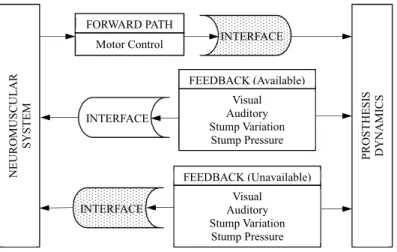
perform similar to a physical arm, elbow and hand, the prosthesis should interface with the neuromuscular system and mimic the closed-loop control non-amputees possess [13]. In an active upper limb myoelectric controlled prosthesis, motor command signals from the central nervous system are used in the forward path. These neuromuscular signals are then utilized to move the prosthesis as the user desires. After completing a desired move, visual, auditory and residual limb

vibration and pressure are used in the feedback signal. These signals feedback to the neuromuscular system to complete the feedback loop. Fig. 2.1 shows a block

diagram of the closed loop control of powered, upper limb prosthesis using

myoelectric control [13]. The shaded blocks in Fig. 2.1 indicate problematic areas in the control system that must be perfected for a more synergetic relationship

between an amputee and the prosthesis.

FORWARD PATH

Motor Control INTERFACE

FEEDBACK (Available) Visual Auditory Stump Variation Stump Pressure INTERFACE FEEDBACK (Unavailable) Visual Auditory Stump Variation Stump Pressure INTERFACE NE UR OM US CU LA R SY ST EM PR OS TH ES IS DY NA M IC S

Many have thought improving the quality of feedback to the central nervous system would be desirable for a prosthesis to be successful. It has been attempted to use proprioceptive and sensory feedback but it has not been accepted due to difficulties in developing a proper interface [38]. However, experimental

investigations demonstrated that this feedback is not necessary for the control of upper limb prostheses [35]. Considering the difficulties in man-machine interface, simple myoelectric control is used to actuate a single device such as a hand or elbow. Using one or two myoelectric channels, the system receives the MES and derives the control signal either as a measure of its amplitude [12] or of the rate of change of its amplitude [10]. Despite the challenges presented in the interfaces, there have been several institutions to successfully implement multifunction prosthesis control.

2.1.1 Weighting Synergistic Muscle Movements - Temple University

Engineers at Temple University with the Moss Rehabilitation Hospital in Philadelphia [15] were one of the first to attempt multifunction control of upper limb prostheses. The team looked to implement control based on myoelectric statistical pattern recognition techniques. They recognized that in able-bodied individuals, elbow movements were completed by several muscle groups acting together. Because movements are a synergistic muscle movement and not a

one-muscle-for-one-muscle control, the goal of their work was to characterize muscle synergies of the arm using pattern recognition.

Their initial work amplified and quantified six channels of MES [15]. The myoelectric activity was monitored during different elbow movements. This activity was analyzed using multivariate pattern recognition techniques in an attempt to optimally distinguish between different desired movements. With normally-limbed subjects who received moderate training producing isometric contractions, the authors reported 92% accuracy for elbow flexion and 97% accuracy for forearm pronation and supination [13].

Further work considered multiple-axis control for an above-elbow amputee where 14 myoelectric sites were used instead of six. After recording data from able-bodied individuals, patterns were classified according to the parameters of their distribution. From these patterns, weighting coefficients were computed to provide maximum separation of the classes. Weighting coefficients were computed for each of the six desired motions and applied to the magnitude of the MES. From these weighing coefficients, it was determined that each movement is distinguishable using a summation threshold. However, the results were not as spectacular as before. Although elbow flexion had a performance accuracy of 97%, humeral rotation had an accuracy of 43% [47]. Unfortunately, the project ultimately demonstrated that

the prosthesis was unable to be controlled properly because the control approach needed a sensory feedback system to be truly effective.

2.1.2 Endpoint Control - University of California, Los Angeles

Engineers at the University of California, Los Angeles (UCLA) sought to refine multifunction control of upper-limb prostheses. Similarly to the work developed at Temple University, the group at UCLA looked to implement control based on myoelectric statistical pattern recognition techniques. This work

originated from studies done by one of the engineers’ previous work with the U.S. Air Force [39] mapping synergistic muscle activity during select arm movements. Instead of mimicking muscle synergies with multiple axes working in unison like the research team at Temple, the UCLA team saw the need for endpoint-based control.

The objective of endpoint control is to relieve the operator of part of the control responsibility. Additionally, because human beings cognitive task space tends to be in Cartesian endpoint coordinates, this type of control provides a more natural control interface. The goal of UCLA’s research was to produce a control algorithm that would allow the user to specify direction and speed of the endpoint along some natural set of coordinates [13]. The team concluded there is a basic limitation on the ability of a user to supply the control information required for adequate performance and no attempt was made to use the MES as the input to the

endpoint control. Instead, a three degree of freedom joystick input was mapped to the appropriate three degree of freedom joint angle vector needed to emulate upper-limb positioning. The control system used the same pattern recognition approach as Temple University, however they looked to provide adaptive mapping to optimize the pattern recognition system for individual users myoelectric patterns. In the end, the team claimed their results were excellent as their prosthesis

completed the proper movement in under 0.5 seconds with two or less erroneous decisions made [48].

2.1.3 Transient Myoelectric Control - University of New Brunswick in Canada

The University of New Brunswick in Canada (UNB) control approach used patterns in the instantaneous MES to define a signature for a particular limb function. More specifically, they looked to implement control based on pattern recognition using the transient MES [13]. The research team at UNB recognized that the complexity of the MES is the root cause for issues with these control systems. Instead of dismissing the idea of using the MES as the input, as the research team at UCLA did in concluding there is not enough control information provided by the user, the team at UNB decided to explore the application of MES as a control input.

After investigation, the team at UNB came to the conclusion that most myoelectric control systems use the steady state myoelectric signals as the control input. The issue with using the steady state signals is that they have little temporal structure due to the active modification of recruitment and firing patterns needed to sustain a contraction [11]. Instead, Hudgins, one of the researchers on the team, investigated the information in the transient burst of myoelectric activity

accompanying the onset of sudden muscular effort. In doing so, Hudgins discovered that the patterns of transient MES exhibit differences in temporal waveforms [24]. From this work, the research group at UNB designed a control system based on the transient response instead of mapping synergistic muscle activity during select arm movements.

The UNB control system used a multilayer perceptron (MLP) ANN to classify values of the time-domain feature set extracted from the single channel MES. Signals from the biceps and triceps were measured, allowing the controller to identify four types of muscle contractions. The block diagram of UNB’s control system can be seen in Fig. 2.2. Utilizing an ANN proves three major benefits: multifunction control from a single site, the control signals can be derived from natural contractions, and conscious effort of the user is minimized [13]. The control system is trained on the distinct MES patterns of the amputee. This information is

then downloaded into the control system which can be used to either control a three degree of freedom prosthetic arm or a virtual arm simulator on a computer.

Figure 2.2: Block Diagram of UNB Control System [13]

2.2 Mechanical and Control Systems of Lower Limb Prostheses

The three universities discussed above looked to implement control based on myoelectric statistical pattern recognition techniques in different ways. Temple University characterized muscle synergies of the arm using MES pattern

recognition. UCLA produced a control algorithm that would allow the user to specify direction and speed of the endpoint along some natural set of coordinates. UCLA abandoned using MES as the inputs and concluded that there is a basic

limitation on the ability of a user to supply the control information required for adequate performance. UNB developed a control system based on the transient response instead of mapping synergistic muscle activity during select arm

movements. Using an ANN, they classified values of the time-domain feature set extracted from the single channel MES.

Despite the success of utilizing EMG signals measured from the residual limb as control commands for active upper limb prostheses, these signals have not been incorporated in the control of active lower limb prostheses. Members of Herr’s laboratory of MIT proposed two EMG-controllers for an active ankle-foot

prosthesis, one using a biomimetic muscle model approach and the other using a neural network approach. They concluded that both controllers demonstrate the ability to predict desired ankle movement patterns qualitatively, with the

biomimetic controller having a smoother movement pattern than the neural network control [5]. Despite these conclusions, these methods for implementing EMG based controllers were not exploited in active lower limb prostheses. The mechanical design, control system and hardware of three academic active lower limb prostheses along with a commercially available passive prosthesis are explored below.

2.2.1 Ossur Propio Foot with Evo¨

The ¨Ossur Proprio Foot with Evo is an active prosthetic device for low to

moderately active transtibial amputees. Motor-powered ankle motion increases ground clearance and reduces the risk of tripping and falling. Due to the motor-powered motion, users are able to navigate different kinds of terrain in a natural and secure way. However, the Proprio Foot is not a fully active transtibial prosthesis. The active components of the prosthesis engage during the swing phase until the ankle reaches a state of maximum dorsiflexion so that the foot has enough clearance. Unlike the Marquette Prosthesis, as well as other fully active prostheses, the joint is locked during the stance phase of swing, not providing any external assistance to the user, thus making it a passive transtibial prosthesis during stance.

2.2.2 BioM - MIT Powered Ankle-Foot Prosthesis

The BioM, first designed in Herr’s laboratory, is an active prosthetic designed to improve amputee walking by decreasing the users metabolic cost of transport. The prosthesis decreased the amputee’s metabolic cost of transport by developing a control system that mimics normal human ambulator stance phase dynamics. The BioM exploits series and parallel elasticity with an actuator to match human-ankle motion with a control system that allows the prosthesis to mimic the target stance phase behavior.

Mechanical Design

The overall mechanical design of the BioM utilizes a parallel spring with a force-controllable actuator with series elasticity to actuate an ankle-foot mechanism. There are five main mechanical elements in the system as shown in Fig. 2.3: a high power output D.C. motor, a transmission, a series spring, a unidirectional parallel spring, and a carbon composite leaf spring prosthetic foot. The first three

components are combined to form a force-controllable actuator, called Series-Elastic Actuator (SEA). The SEA provides force control by regulating the extent to which the series spring is compressed. Using a linear potentiometer, the BioM can obtain the force applied to the load by measuring the deflection of the series spring.

The BioM requires a high mechanical power output as well as a large peak torque. Due to the demanding output torque and power to provide the active push-off during Powered Plantarflexion (PP), the parallel spring shares the payload with the force-controllable actuator. The reduction of the payload experienced by the SEA also allows for a smaller transmission ratio to be used. The elastic leaf spring foot is used to emulate the function of a human foot that provides shock absorption during foot strike, energy storage during the early stance period, and energy return in the late stance period [4].

Control System

The control system of the BioM mimics a normal human beings stance phase behavior. The control system consists of an FSC to replicate the target stance behavior and three types of low-level servo controllers to support basic ankle behavior. The overall architecture of the control system is shown in Fig. 2.4.

Figure 2.4: BioM Controller Architecture [4]

The FSC was implemented to replicate the target ankle behavior. It is comprised of two parts: stance phase control and swing phase control. For stance phase control, three states were designed to mimic natural walking [4]. The first state, Controlled Plantarflexion (CP), begins at heel strike and ends at mid-stance. The second state, Controlled Dorsiflexion (CD), begins where CP left off and ends right before Powered Plantar (PP) or toe-off. The final state, PP, begins only if the measured total ankle torque is larger than the predefined torque threshold. If this is not satisfied, the prosthesis remains in CD until the foot is off the ground. For swing phase control, three states were also designed to ensure foot clearance and preparation for the next gait cycle. The first state, Swing Phase 1 (SW1), begins at

toe-off and ends after a specified time. The second state, Swing Phase 2 (SW2), begins right after SW1 and finishes when the foot reaches zero degree. The final state, Swing Phase 3 (SW3), runs for a specified time period determined

experimentally to ensure the system is ready for heel-strike [6].

As shown in Fig 2.4, the three types of low-level servo controllers are an impedance controller, a force controller and a position controller. The torque controller was designed to provide the offset torque and facilitate the stiffness modulation. This controller uses force feedback, estimated from the series spring deflection, to control the output joint torque of the SEA. The force controller utilizes a PD controller to regulate the input voltage to the motor amplifier and allow the prosthesis to bounce back if it hits a hard boundary due to large impact force seen in the spring.

The impedance controller modulates the joint stiffness of the SEA.

Impedance control regulates a dynamic relationship between manipulator variables such as the ratio of position and force rather than just control these variables alone. In the BioM impedance controller, a dynamic relationship is established between the output torque and the ankle joint angle. The impedance controller uses the ankle angle, fed back via a position encoder, to increase the output joint impedance. Due to the complexity of the ankle joint, it is crucial to take into account major components of impedance, such as the effective mass, inertia, damping and stiffness,

for specific tasks and movements to be completed as desired [30]. In order to avoid the effect of intrinsic impedance, the torque controller was incorporated into the impedance controller. The actual output consists of desired output impedance due to the controller plus that due to the mechanism.

A standard PD controller was implemented as a position controller. Its purpose is to control the equilibrium position of the foot during swing phase. This

control is similar to that of the ¨Ossur Proprio Foot with Evo and ensures the foot

clears the ground to avoid tripping or falling. With PD control, however, the BioM is able to prepare for Controlled Plantarflexion (CP) and the next stance phase.

System Hardware

The BioM electronic system is shown in Fig. 2.5. It contains an onboard computer, PC/104, with a data acquisition card, power supply and motor amplifiers. The system is powered by a 48V, 4000mAh Li-Polymer battery pack. A custom breakout board interfaced the sensors to the D/A board on the PC/104 as well as provided power to the signal conditioning boards. The PC used was a MSMP3XEG PC/104. The PC/104 systems are intended for applications where a small, rugged computer system is required [34]. It was fitted with a PENTIUM III 700 MHz processor. A PC/104 multifunctional I/O Board from Sensory Co. was connected to the PC/104, containing 8 analog inputs, 2 analog outputs and 4 quadrature encoder

counters. The system runs in real-time using the MATLAB xPC real-time kernel and Simulink. The Simulink model was compiled on the host PC using MATLAB RealTime Workshop and a C++ compiler created executable code. The system uses a linear potentiometer to measure the displacement of the series springs, a

quadrature encoder to measure the joint angle of the prosthesis ankle and six capacitive force transducers, two beneath the heel and four beneath the forefoot.

Figure 2.5: Computer System of BioM [4]

2.2.3 SPARKy 3 - ASU Powered Ankle-Foot Prosthesis

SPARKy 3, short for Spring Ankle with Regenerative Kinetics, was designed and implemented by Sugar’s laboratory at Arizona State University. This active prosthesis attempts to bring full able-bodied ankle function to transtibial amputees.

The first generation, SPARKy 1 [20], used regenerative kinetics to accurately and efficiently reproduce the human gait cycle. The second generation, SPARKy 2 [7], enhanced the mechanical and electrical system of the first generation. The chief goal of the third phase of SPARKy 3 was to build a more dynamic prosthesis, i.e., one that moves in two directions instead of one, without sacrificing size, weight or performance compared to the previous generations [7].

Mechanical Design

In order to minimize the required peak power supplied by the motor, SPARKy utilizes a robotic tendon shown in Fig. 2.6 [23]. This device includes a linear actuator in series with a spring and a small, lightweight, low energy motor that is used to adjust the position of the helical spring. The robotic tendon design was developed to mimic the elastic nature of the human muscular system in minimizing the work and peak power. The simple inclusion of a spring to a linear actuator can provide energy and power savings to the prosthesis. The spring releases its stored energy to provide most of the peak power required during the powered plantar phase of gait. In the simple series model of SPARKy, the keel and the robotic tendon springs are in series. The two degrees-of-freedom model is shown in Fig. 2.7.

Figure 2.6: Robotic Tendon Model: Motor and Spring in Series [23]

Figure 2.7: Two Degrees-of-Freedom SPARKy Model [21]

The goal of SPARKy 3 was to achieve running and jumping. Thus a second DC Powermax 30 motor had to be introduced to the system in order to increase power capacity. The SPARKy 3 CAD model is shown in Fig. 2.8. With regards to walking, the two motors work together either compressing or extending the two helical springs. For example, during powered push-off, the motors move together releasing the energy in the springs [7].

Control System

In order to control the system shown in Fig. 2.8, Arizona State uses the tibia angle profile for able bodied human gait. This relationship between tibia angle and percent gait cycle analyzed for different stride lengths. These profiles are seen in Fig. 2.9. From this relationship, it was observed that each different stride length produces an almost identical curve, only scaled by some function of stride length. They created a control system that sought to find a measurable variable to determine a mathematical relationship between the tibia angle and ankle angle. Ultimately, the tibia global angle was chosen due to this relationship and how easy it is to measure this angle by attaching a sensor to the prosthetic device [22, 23].

The angular velocity of the shank is measured using a rate gyro. The ankle

angle and ankle moment is calculated via published kinematic data as shown in Fig. 2.9. With the moment and angle, they are then able to calculate the nut reference for the robot [23]. The major advantage the control algorithm for ASU has is that it uses a vast amount of published data of ankle angles, moments, tibia angular

velocity, etc. such that the prosthesis is adaptive to its user despite of height or weight.

Figure 2.9: Tibia Angle Profile vs Human Gait. Each curve represents a different stride length [22]

System Hardware

The SPARKy 3 electronic system can be seen in Fig. 2.10. SPARKy 3 utilizes a simple series model with the Maxon RE 40 motor with a planetary gear box, Maxon GP42, having a 4.3:1 gear ratio. From Fig. 2.8, one can see the mechanical system utilizes two EC Powermax 30 motors, roller screws, a pylon,

L-arms and two helical springs. It is controlled in real time using Real Time Workshop and Simulink. The model is compiled onto the embedded target PC running the xPC target operating system. Advantech’s 650 MHz PC/104 with 512 MB on board memory is selected to run the system. A multifunctional I/O board from Sensoray Co., Model 526, is connected to the PC/104 via ISA Bus, controls the motors with encoders as the feedback devices. There are three sensors used on the system: one encoder at the motor, another encoder at the ankle joint, and an optical switch embedded at the heel. As stated previously, the controller has a predetermined gait pattern based on able-bodied gait data and kinetic analysis expressed as a time-based function embedded in the controller [21].

2.2.4 Vanderbilt University Powered Ankle and Knee Prosthesis

A transfemoral prosthesis was developed and implemented by Goldfarb’s lab at Vanderbilt University. Unlike the work done by MIT, ASU and in this thesis, Vanderbilt designed a prosthesis that consists of both a powered knee and ankle. Prior to the work of Goldfarb and Sup [45], a powered knee transfemoral prostheses and powered ankle transtibial prostheses did not exist as one entity, only powered knee or powered ankle prostheses. The goal was to create a prosthesis with the capability to deliver power at the knee and ankle joints to enable the restoration of biomechanically normal locomotion [42].

Mechanical Design

The driving mechanisms of the powered ankle and knee prosthesis are two slider-crank mechanisms, as shown in Fig. 2.11 and Fig. 2.12: one located at the knee and one locating at the ankle. The first generation of the prosthesis utilized two pneumatic actuators to drive the system. However, due to the expense as well as practicality of a pneumatic actuator, the second generation looked to move from a pneumatic system to an electrical system. The second-generation device consists of a Maxon motor for each actuation unit. The motor is connected to a ball screw assembly that actuates the prosthesis. The kinematic configuration of the actuators was selected via a design optimization to minimize the volume of the actuators. The

active joint torque specifications for the prosthesis were based on the torque/angle phase space required for an average user for fast walking and stair climbing, as derived from body-mass-normalized data from Winter et al. [41, 42].

Figure 2.11: Slider Crank Configuration [41]

Control System

The powered knee and ankle prosthesis has three activity modes: walking, standing and sitting. It has control algorithms for transition from one activity mode to another as well as control algorithms within each activity mode. The control structure is shown in Fig. 2.13 [43]. It consists of high-level controllers, middle-level controllers and low-level controllers. The highest level consists of three parts: the activity-mode intent recognizer, the cadence estimator and the slope estimator. The latter two estimate the slope and cadence during walking to adjust the parameters of the walking-mode controller. The activity mode recognizer recognizes one of several activity modes, whether its walking, running, sitting, standing, climbing, etc. and switches to the appropriate middle level controller.

2.2.5 System Hardware

Figure 2.14: Embedded System Framework [41]

The self-contained version of the knee and ankle prosthesis includes an embedded system which can be controlled from a laptop via MATLAB Simulink or untethered using an 80MHz, 512 kB Flash, 32 kB RAM PIC32 onboard

microcontroller. In the tethered version, the prosthesis is controlled via MATLAB Simulink RealTime Workshop. In the untethered version, the microcontroller

performs the servo and activity controllers of the prosthesis. It is actuated with two Maxon EC30 Powermax brushless motors, powered by a lithium polymer

battery [44]. The prosthesis integrates a custom load cell to measure the

gages to measure the ground reaction force at the heel and ball of the foot, and precision potentiometers and load cells to measure joint positions and torques, respectively [43]. The embedded system framework is shown in Fig. 2.14.

2.3 Summary

While the prostheses mentioned in this chapter look to restore natural walking of amputees, their control systems fall short when the terrain changes abruptly. These prostheses struggle when amputees transfer from flat ground to climbing a flight of stairs or going down a flight of stairs. This is because these control systems are unable to properly predict when a change in the amputees walking environment is about to occur. By using EMG information measured at the residual limb, this research looks to implement a neural network control approach to predict ankle movement, ultimately making a more natural, smooth stride for normal and changing terrains.

2.4 Marquette Prosthesis

The Marquette Prosthesis was able to meet the published ankle angle and torque when tested on human subjects. However, the Marquette Prosthesis

exploited the issue with an FSC - it is not robust enough to consider more normal or abnormal situations such as a transition from walking on an incline or from walking

to running [40]. Unfortunately, due to the reactionary nature of an FSC, an FSC is not robust enough in these transition phases. The three schools discussed above, MIT, ASU and Vanderbilt, were able to get their prostheses to run and walk up inclines, however the initial step to transition to running or climbing were awkward for the amputee due to the FSC. Because the controller proposed in this thesis received the predicted stiffness of the ankle from an ANN [14] and controls the stiffness of the ankle continuously, the issue experienced by an FSC is eliminated.

CHAPTER 3

Dynamic Model and Simulation

In this chapter, the updated dynamic model of the Marquette Prosthesis II will be presented and discussed followed by the simulation results. Creating a dynamic model of any system is critical to understand how a system will behave and to assess the validity of a system. A model offers insight and saves time and money by ensuring a system performs as expected and avoids potential unseen problems. With this goal in mind, Sun created a two-phase model of the Marquette Prosthesis and simulated it using Simulink and SimMechanics before implementing its

controller [40]. Unfortunately, this model is insufficient for this thesis due to changes in the mechanical design as well as changes in the type of controller implemented.

Because the Marquette Prosthesis controller in [40] was an FSC which

changed controller type based on whether the amputee was in stance or swing mode, two separate models were created: one for swing and one for stance [40]. With the Marquette Prosthesis II, the controller drives the ankle continuously regardless of the stage or type of gait. The ANN will provide a desired torque and position regardless of the stage of gait [14]. Thus, the model needed only to have one stage.

fidelity. There were two major outcomes of this model and simulation. The first was to determine the PI parameters for the motor position to ensure the relationship between the ankle position and torque was satisfied. This simulation provided a benchmark for the final PI parameters used in the physical control system. The second was to determine an appropriate spring constant for the linear spiral torsional spring. In order to implement stiffness control, the linear spiral torsional spring was redesigned to be in series with the four-bar mechanism. With the spring in series with the four-bar mechanism, the desired spring constant to meet the torque requirements of the ankle needed to be investigated.

3.1 Four Bar Mechanism Analysis

A model of the Marquette Prosthesis II can be seen in Fig. 3.1. In this model, the motor moves independently of the mechanism. The ANN will receive EMG activity and the current position of the ankle and output the desired position,

θ, and torque of the ankle,τankle [14]. For the dynamic model, published data was

used to determine the desired position and desired torque of the ankle [46]. The

angular position of the motor shaft, ψ, was determined from the ratio of the desired

position of the ankle,θ, and desired torque of the ankle, τankle. However, the motor

shaft angular position, ψ, relies heavily upon the input angle of the four-bar

φ, was derived from the desired angle of the ankle, θ, using kinematic relationships.

Furthermore, the torque provided by the spring,τspring was derived from the

published torque at the ankle, τankle, using the quasi-static relationship.

Torsional Spring Knee Foot Ankle

φ

θ

A

B

C

D

Figure 3.1: Model of the Marquette Prosthesis II

3.1.1 Kinematics

The first step in creating the model was to determine the kinematic

relationship between the angles of the four-bar mechanism. A sketch of the four-bar mechanism with the angles labeled and the coordinate system defined is shown in Fig. 3.2 and is repeated in Fig. A.1 and Fig. B.1. Because the position of the motor is independent of the mechanism, a classical vector loop approach was used to

the ankle,θ. As such, the derivation was standard and follows the approach found in Norton’s Design of Machinery and is repeated in this thesis in Appendix A for

completeness [32].1

φ

θ

X

Y

α

Figure 3.2: Sketch of the Four-Bar Mechanism

From Appendix A, the solution for the input angle of the four-bar

mechanism, φ as a function of the ankle angle, θ, was found by using the quadratic

equation: φ1,2 = 2 arctan( −B±√B2_−4AC 2A ) (3.1) where: A= cosθ−K1−K2cosθ+K3 B =−2 sinθ C =K1−(K2+ 1) cosθ+K3

Equation 3.1 has two solutions that may be of three types: real and equal, real and unequal, or complex conjugates. If the solutions are real and equal, then the mechanism is in a singular configuration [1]. For this work, the singular position is to be avoided in the workspace. If the solutions are complex, then the desired angle is impossible to reach. In other words, the link lengths are not capable of being connected at that angle. If the solutions are real and unequal, then these results are two different solutions for the two assembly modes. Thus, the result from Equation 3.1 should be real and unequal. From these two possibilities, the

appropriate assembly solution was selected depending on whether or not the configuration of the linkages is closed or open [32].

From Equation 3.1, the desired input angle of the four-bar mechanism, φ,

was determined for a given ankle angle, θ. Because the spring was moved in series

the position of the motor, ψ, input angle of the four-bar mechanism, φ, spring constant, Kspring, and the torque provided by the spring, τspring. This relationship is

shown in Equation 3.2. Therefore, before controlling the position of the motor, ψ,

the torque provided by the spring was determined using quasi-static relationships.

ψ = τspring

Kspring

+φ (3.2)

3.1.2 Quasi-statics

The desired torque provided by the spring was determined using quasi-static relationships based on the desired output torque at the ankle and current pose of the prosthesis. Quasi-statics is the ability to analyze a dynamic system statically as the inertial force is very small compared to the torque exhibited [1]. In other words, the dynamic forces are small compared to the static forces. According to

Bergelin [8] and further shown by Malak [29], the dynamic forces and gravitational forces in this application are small and the system can be modeled quasi-statically. With this approach, a static analysis was performed at different poses of the mechanism. The quasi-static analysis can be found in Appendix B.

The set of 13 equations and 13 unknowns found in Appendix B fully describe the statics of the mechanism when used in conjunction with the kinematic

desired torque provided by the spring, τspring. The desired position of the motor, ψ,

was determined using the relationship shown in Equation B.13.

The software must compute the desired position of the motor based on the desired position of the ankle in real time. Due to this, the simplified model shown via the quasi-statics was utilized in the controller to quickly calculate the desired angle.

3.2 Simulink Model

With the dynamic relationships established, the full dynamics of the plant were modeled and simulated. This model, while not applicable to the real time implementation, was used to validate the controller for robustness. Due to their ability to accurately model systems with many degrees of freedom due to their ability to solve several ODEs simultaneously, MATLAB and Simulink were used to create a higher fidelity model. In this thesis, the primary purpose of using a

Simulink model was to design a robust controller. Although it has been proven that the dynamic forces and gravitational forces are small in this application [8, 29], simulating the system with these forces ensured the actual stiffness met the desired stiffness.

in Appendix C. This desired ankle position with respect to time is shown in Fig. 3.3 and is based on published data [18, 46].

0 0.1 0.2 0.3 0.4 0.5 0.6 0.7 0.8 0.9 1 time (s) -25 -20 -15 -10 -5 0 5

10 Published Desired Ankle Position Versus Time

Figure 3.3: Published Position Versus Time According to Winter [46]

3.2.1 Dynamic Simulation and PI Tuning

With the system modeled as shown in Fig. C.1, the PI gains of the motor controller were determined such that the desired stiffness of the ankle was met. Note that because the mechanism is a four-bar mechanism, the input/output relationship is nonlinear. Typically, the PI parameters are tuned by linearizing the model from the plant and then determining the parameters from the derived model. Due to the nonlinearity of the four-bar mechanism, a modified Ziegler Nichols approach was used on the model to obtain the PI parameters.

There are typically two Ziegler-Nichols methods used to tune PI controllers: the Ultimate Cycle Method and the Process Reaction Method. The Process

Reaction requires a step change of the controller’s output that alters the controlled variable. Based on the shape and magnitude of the controlled variable’s reaction curve in reference to the step change, the response is linearized to obtain values to be used in mathematical formulas to calculate the control gains [27]. As the four-bar mechanism is nonlinear, the Ultimate Cycle Method was implemented on the Simulink model. The Ultimate Cycle Method requires one to set up a

proportional controller and slowly increase the gain until the system has sustained oscillations. Once sustained oscillates have been achieved, the proportional gain used to obtain sustained oscillations is used to calculate approximate gains for a PI controller. From here, the gains are fine-tuned until the actual position correlates to the desired position. The final PI gains that yielded the position response shown in Fig. 3.4 are seen in Table 3.1.

Table 3.1: Final Parameters for Tuned Controller Parameters P (unitless) I (s−1) Tuned Value 416 159 An kl e An gl e (° )

Figure 3.4: Desired Ankle Angle versus Actual Ankle Angle

3.2.2 Investigation of Linear Spiral Spring

The Marquette Prosthesis was developed and optimized such that the spring would provide the required ankle torque with the assumption that the spring was fixed to the grounded link [8], i.e., in parallel with Joint A. Due to this assumption, previous models with parallel springs are not valid when trying to implement stiffness control. Stiffness control requires the linear spiral torsional spring to be in series with the motor and four-bar linkage as shown in the Simulink model in

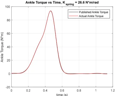
Appendix B. This new model along with the limitations of the mechanism, motor, and gearbox can be used to select a spring constant such that the torque of the ankle meets the desired torque of the ankle. Fig. 3.5 shows the desired ankle torque compared to the actual ankle torque with the old spring, now in series, as

determined by the Simulink model.

Figure 3.5: Desired Ankle Torque versus Actual Ankle Torque with Original Spring

3.2.3 Effect of Spring Constant on Output Torque

As an attempt in finding an adequate spring constant, a few limiting cases of spring constants were attempted. Fig. 3.6 shows the ankle torque with a spring constant of 26.6 N*m/rad compared to the motor torque with a spring constant value of 13.3 N*m/rad, 6.7 N*m/rad and 2.66 N*m/rad, half, quarter and a tenth of

the original spring constant value, respectively, to investigate the effect of the spring constant on the output torque.

Figure 3.6: Effect of Spring Constant on Motor Torque

There is little to no effect of the spring constant on the motor torque because the torques are consistent regardless of the spring constant as shown in Fig. 3.6. However, the selection of a spring is vital and an engineering judgement should be made in selecting the appropriate spring constant. For instance, a spring with a lower spring constant will cost less, will weigh less and will reduce the noise, i.e., sound from the motor. However, there is a limitation of a spring with a low spring constant. A lower spring constant will require the motor to move faster so that the desired ankle torque and position are met.

3.2.4 Motor Torque and Speed Capabilities

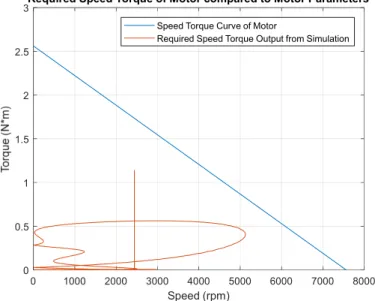
With the effect of the spring constant on the output torque investigated, it was important to ensure the required torque and speed curves fall under the speed torque curve for this motor. Fig. 3.7 shows the motor speed torque curve with a spring constant of 26.6 N*m/rad from Simulink, where the Maxon RE-40 Brushed DC motor has a no-load speed of 7590 rpm and a stall torque of 2.56 N*m. From Fig. 3.7, it is clear that the motor should have no issue meeting the speed torque requirements of the prosthesis. Unfortunately, due to the motor’s speed and torque, its efficiency drops below 50%. When the motor is running below 2000 rpm or above 0.2 N*m, its efficiency drops off [21].

0 1000 2000 3000 4000 5000 6000 7000 8000 Speed (rpm) 0 0.5 1 1.5 2 2.5

3Required Speed Torque of Motor compared to Motor Parameters

Speed Torque Curve of Motor

Required Speed Torque Output from Simulation

3.2.5 Final Spring Selection

The model shows that the spring does not have much of an effect on the motor and the motor can meet the speed and torque requirements of the system. As with any model, these results should be validated with the physical system. The effect of changing the spring constant on the physical system is something that will be revisited in the future work of this thesis. For this work however, the original spring with a spring constant of 26.6 N*m/rad was selected due to the constraints of this project.

CHAPTER 4

Mechanical System Redesign

The Simulink model of the Marquette Prosthesis II shows that stiffness control is feasible, but some mechanical changes were made before implementation. The design of the Marquette Prosthesis utilized a linear spiral torsional spring in parallel with a four-bar mechanism to mimic the complex nonlinear response of the foot and ankle as shown in Fig. 4. Because stiffness control requires a relationship

between the motor position, ψ, the torque of spring,τspring, and the input angle of

the four-bar mechanism, φ, the linear spiral torsional spring was moved in series

with the motor and link 3 as shown in Fig. 4. Therefore, to move the spring from being in parallel to series with link 3 and the motor, link 3 was redesigned. Due to cost and manufacturing constraints, the Marquette Prosthesis II was constrained by the linear spiral torsional spring and link lengths chosen for the Marquette

Motor

Figure 4.1: Model of Marquette Prosthesis with Spring in Parallel with the Motor Adopted from [40] Torsional Spring Knee Foot Ankle φ θ A B C D

4.1 Redesign of Link 3 to move spring in Series

The Marquette Prosthesis had one end of link 3 fixed to the motor shaft and the center of the spring slotted into the motor shaft. A mount, shown in Fig. 4.3, connected the outer hook of the spring to a bolt which threaded into the mount. The two slots of the block were fit around the ground link and were secured via a bolt; therefore, the spring was grounded. To move the spring in series with the motor and link 3, this mount was removed.

Figure 4.3: Mount that Connects the Spiral Torsion Spring to Link 0

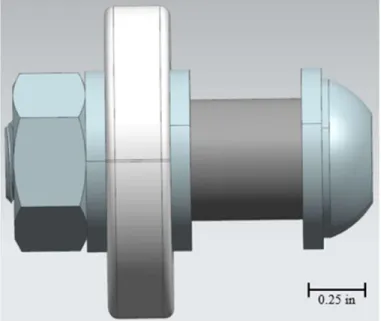
The new design of link 3, shown in Fig. 4.4, was a rectangular bar with rounded edges containing three holes, two thru holes and one threaded hole, for attachment to the motor, spring and link 2. The new design required a bearing to connect link 3 to the motor shaft to rotate freely about the motor shaft. The center of link 3 was designed to press fit a bearing into a thru hole. Because the redesign of link 3 was constrained by the size of the spring and a bolt was used to connect the

spring to the grounded mount shown in Fig. 4.3, the distance from the bearing hole to the threaded hole was designed to be equal to the distance from the center of the spring to the center of the outer loop of the spring, shown in Fig. 4.5. The center of the spring was then slotted into the motor shaft and a bolt connected the outer loop of the spring to link 3. A nut was then threaded onto the bolt to secure the

connection between the spring and link 3. A side view of this assembly is shown in Fig. 4.6, where the linear spiral torsional spring is black and the link is white. Because the link length was constrained by the Marquette Prosthesis design, the distance from the center of the bearing to the center of the other thru hole was equal to the length of link 3. A dowel pin was then press fit into this second thru hole to connect link 3 to link 2.

Figure 4.5: Linear Spiral Torsional Spring

4.1.1 Press Fit Analysis

ANSYS 19.0 was used to ensure the stress and deformation due to the press fit would not cause the part to fail. After the dowel pin and link were imported from NX 10.0 as an assembly, the appropriate material was assigned to the pin and link. The pin was assigned alloy steel as its material and the link was assigned Aluminum 7076-T6 as its material. A frictional contact was established between the surface of the dowel and the surface of the hole of the press fit. In the settings of the frictional contact, the normal stiffness factor was changed manually from 1.0 to 0.1 and the stiffness was updated on each iteration since the stiffness will change as the dowel pin is pressed into the hole. In the geometric modification section of the contact, the interface treatment setting was changed to “Add Offset Ramped

Effects” as this appropriately models the expansion of the hole as the dowel is press fit. The mesh was original sized to have an element size of 1.0 mm and was further refined to 0.5 mm to validate the results. The sides of the link were then fixed and the analysis settings were altered such that the solution would converge, outputting the deformation and equivalent stress.

The deformation and equivalent stress due to the press fit are shown in Figs. 4.7 and 4.8, respectively. From the Finite Element Analysis, the maximum

deformation was 0.0216 mm and the max von Mises stress was 415 MPa compared with a yield strength of 470 MPa. Although the resulting stress is close to the yield

strength of Aluminum 7076, is it still less than the yield strength. This result, along with only 0.0216 mm of deformation, inferred that the press fit can be completed without failure.

Figure 4.7: ANSYS Deformation Results

CHAPTER 5

Control System Architecture and Implementation

With the appropriate mechanical changes made on the Marquette Prosthesis as described in Chapter 4, the controller was implemented. In this chapter, the architecture of the control system is outlined and details of the implementation are provided.

5.1 Overall Control System Architecture

There were two main components to the architecture of the control system developed for the Marquette Prosthesis II: the ANN and the stiffness controller. The ANN will provide the desired ankle position and torque while the stiffness controller controlled this stiffness via the motor. Because the ANN was not fully developed at the time of this work, published data was used to provide the desired

position, θ, and torque of the ankle, τankle. From the desired position and torque of

the ankle, the kinematics and quasi-statics as discussed in Chapter 3 and Appendices A and B were computed to determine the desired motor position.