Automatic identification of land cover types from satellite data with machine learning techniques

(1)

Automatic identification of land cover types from

satellite data with machine learning techniques

University of Helsinki

Riikka Huusari

(2)

Faculty of Science Department of Mathematics and Statistics Riikka Huusari

Automatic identification of land cover types from satellite data with machine learning techniques Applied Mathematics

Master’s thesis May 2016 42 p.

Machine learning, satellite data, support vector machines, clustering

This study is part of the TEKES funded Electric Brain -project of VTT and University of Helsinki where the goal is to develop novel techniques for automatic big data analysis. In this study we focus on studying potential methods for automated land cover type classification from time series satellite data. Developing techniques to identify different environments would be beneficial in monitoring the effects of natural phenomena, forest fires, development of urbanization or climate change.

We tackle the arising classification problem with two approaches; with supervised and unsuper-vised machine learning methods. From the former category we use a technique called support vector machine (SVM), while from the latter we consider Gaussian mixture model clustering technique and its simpler variant, k-means.

We introduce the techniques used in the study in chapter 1 as well as give motivation for the work. The detailed discussion of the data available for this study and the methods used for analysis is presented in chapter 2. In that chapter we also present the simulated data that is created to be a proof of concept for the methods. The obtained results for both the simulated data and the satellite data are presented in chapter 3 and discussed in chapter 4, along with the considerations for possible future works. The obtained results suggest that the support vector machines could be suitable for the task of automated land cover type identification. While clustering methods were not as successful, we were able to obtain as high as 93 % accuracy with the data available for this study with the supervised implementation.

Tiedekunta/Osasto — Fakultet/Sektion — Faculty Laitos — Institution — Department

Tekijä — Författare — Author Työn nimi — Arbetets titel — Title Oppiaine — Läroämne — Subject

Työn laji — Arbetets art — Level Aika — Datum — Month and year Sivumäärä — Sidoantal — Number of pages Tiivistelmä — Referat — Abstract

Avainsanat — Nyckelord — Keywords

Säilytyspaikka — Förvaringsställe — Where deposited

(3)

Matemaattis-luonnontieteellinen Matematiikan ja tilastotieteen laitos Riikka Huusari

Automaattinen maanpeittotyyppien luokittelu sateliittidatasta koneoppimisen menetelmillä Soveltava matematiikka

Pro gradu -tutkielma Toukokuu 2016 42 s.

Koneoppiminen, sateliittidata, tukivektorikoneet, klusterointi

Tutkielma on osa TEKES-rahoitteista VTT:n ja Helsingin yliopiston Electric Brain -projektia, jon-ka tarkoituksena on kehittää tekniikoita automaattiseen suurien datamäärien käsittelyyn. Tämä työ keskittyy tutkimaan potentiaalisia menetelmiä automaattiseen maanpeittotyyppien tunnistukseen aikasarjaluonteisesta sateliittidatasta. Tällaiset automaattiset seurantamentelmät olisivat hyödylli-siä erilaisten luonnon- ja muiden ilmiöiden tarkkailuun; mahdollisia seurantakohteita ovat esimer-kiksi metsäpalot, urbaanien alueiden kehittyminen ja ilmastonmuutoksen aiheuttamien muutosten tarkkailu.

Lähestymme luokitteluongelmaa kahdesta lähtökohdasta: ohjatun ja ohjaamattoman koneop-pimisen menetelmillä. Ensimmäisestä kategoriasta käytämme tekniikkaa nimeltä tukivektorikone, kun taas jälkimmäisessä keskitymme klusterointiin Gaussisilla sekoitemalleilla ja niiden yksinker-taisemmalla versiolla, k-means -menetelmällä.

Esittelemme työssä käytettävät tekniikat ja motivaatiota työlle kappaleessa yksi. Tarkemmin nämä tekniikat käsitellään kappaleessa kaksi, jossa myös esitellään työssä käytettävä data, sekä simuloitu data joka on luotu tekniikoiden toimivuuden testaamiseksi. Tulokset sekä simuloidulla että oikealla datalla esitellään kappaleessa kolme. Keskustelemme tuloksista ja mahdollisista laa-jennoksista työlle kappaleessa neljä. Saadut tulokset viittaavat siihen, että tukivektorikone voisi olla soveltuva menetelmä tämäntyyppiseen sateliittidatan analysointiin. Korkein saavutettu tark-kuus tukivektorikoneilla maanpeittotyyppejä luokitellessa oli 93 %, joka oli huomattavasti parempi kuin klusterointimenetelmillä saavutetut tulokset.

Tiedekunta/Osasto — Fakultet/Sektion — Faculty Laitos — Institution — Department

Tekijä — Författare — Author Työn nimi — Arbetets titel — Title Oppiaine — Läroämne — Subject

Työn laji — Arbetets art — Level Aika — Datum — Month and year Sivumäärä — Sidoantal — Number of pages Tiivistelmä — Referat — Abstract

Avainsanat — Nyckelord — Keywords

Säilytyspaikka — Förvaringsställe — Where deposited

(4)

Acknowledgements

This work was funded by Finnish Technology Agency (TEKES); the decision number is 528/31/2015.

First and foremost I want to thank professor Samuli Siltanen for supervising this work and giving the opportunity to make the thesis for Electric Brain project. Big thank you to Oleg Antropov from VTT for providing the data for this study. I thank also South Savo Regional fund of Finnish Cultural Foundation for funding my thesis work.

(5)

Chapter 1 Introduction

This study is part of the Electric Brain -project of VTT and University of Helsinki where the goal is to develop novel techniques for automatic big data analysis. Developing these adaptive and automated self-learning methods is important as the amount of satellite data collected increases. These methods would help reducing the expert manual work and at the same time they would speed up the analysis process decreasing the subjectivity of the analysis.

We present here potential methods for automated classification of satellite time series data into different land cover types. This is important in monitoring the environment. From satellite images one can study the changes occurring in forests, lakes, cities or for example deserts, not to mention the polar ice cover. Developing techniques to identify these different environments would thus be very beneficial in monitoring the effects of natural phenomena, forest fires, development of urbanization or climate change. The goal of this study is to present potential methods for the classification rather than finished large scale products.

As there is a lot of satellite data available one does not need to restrict the classification problem to one image. Instead, one can collect a series of images over the same site and form a time series on which the classification is then performed. This is advantageous as the robustness of the classification increases as more data is used. Mistakes, errors or bad conditions at the time of imaging will not have as great effect in the final results. Also in the case of land cover type identification in the conditions of Finland the natural variations over time can be useful.

We tackle the arising classification problem with two approaches; with supervised and unsupervised machine learning methods. In supervised machine learning the algorithm receives some data and additional knowledge of these data points, usually the class labels. Based on these known qualities of the data the algorithm tries to find the differences between the data points belonging to different classes. If the data is representative and

(7)

this is done well, the classification can be used to classify previously unseen data of the classes. Here the main supervised classification tool is a support vector machine.

Support vector machines are a very powerful tool for classification. They were invented by Boser, Guyon and Vapnik et al. in 1992, but the theory and features had been used since 1960 by Vapnik and others [14]. Support vector machines have been successfully applied in many fields, for example bioinformatics, computational linguistics and image recognition [14]. Support vector machines search for a border in the data which divides it into the different classes. What makes them so flexible is the usage of a kernel trick that allows one to perform nonlinear classification with easier linear methods.

As supervised machine learning methods utilize the class knowledge of available data, unsupervised machine learning techniques are can be used in situations when there is no knowledge of the class labels the data might have. In this kind of learning the goal is to find some interesting structure purely based on the observed data. We use unsupervised clustering methods, namely Gaussian mixture models and its simpler implementation k-means, to search for structure in the satellite time series data.

One of the first examples of mixture models is in the work of Karl Pearson from 1894 [12], but the expectation maximization algorithm for mixture models that enabled feasible calculations was invented much later. It was first published in a seminar paper by Dempster, Laird and Rubin (1977) although this kind of method had also been discussed earlier [12].

Although in this study clustering methods are used for data classification there are many other usages for them. They are often used in data compression or feature selection [4].

The detailed discussion of the data available for this study and the methods used for analysis is presented in chapter 2. In the chapter we also present the simulated data that is created to be a proof of concept for the methods. The obtained results for both the simulated data and the satellite data are presented in chapter 3 and discussed in chapter 4, along with the considerations for possible future works. The obtained results suggest that the support vector machines could be suitable for the task of automated land cover type identification. While clustering methods were not as successful, we were able to obtain as high as 93 % accuracy with the data available for this study with the supervised implementation.

(8)

Chapter 2 Materials and methods

This chapter describes the data used in this study and the methods for identifying the land cover classes. We will first introduce simulated data used as a proof of concept, and then the satellite data that the actual analysis is performed on. Clustering methods are introduced in section 2.2, and support vector machines in section 2.3.

2.1 The Data

2.1.1 Simulated data

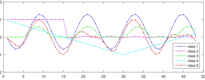
Simulated data was created for this study to serve as a proof of concept for land cover type classification. As in the actual time series data from the satellite images, the dimension-ality of each object is 48. Also similarly there are five different classes for classification; the template functions are introduced in figure 2.1. The 2000 data instances from each class were created from the templates by adding normally distributed random noise.

2.1.2 Satellite data

This study uses data obtained from satellite images. The satellite in question is a C-band Synthetic Aperture Radar (SAR) satellite Sentinel 1 of ESA from Copernicus Earth ob-servation programme [1]. In contrast to some satellites that use starlight or light from our sun, the SAR is an active system that transmits a beam of radiation in the microwave region of the electromagnetic spectrum [2]. This means that Sentinel 1 can take images independent of the time of the day or the cloud cover. This is a clear advantage when considering the quality of the data as there is likely to be less outliers or other distur-bances that cloud cover or the timing of imaging could cause. Sentinel 1 measures two polarizations that scatter or reflect back to it.

(9)

0 5 10 15 20 25 30 35 40 45 50 -2 -1 0 1 2 class 1 class 2 class 3 class 4 class 5

Figure 2.1: The template functions for the simulated data.

A SAR is a kind of radar that uses its own motion to simulate more accurate radar [2]. It uses signal processing techniques to obtain images of better resolution than just a physical antenna aperture. SAR takes images in succession of some single area while flying over it obtaining a combination of those images.

The data in this study is obtained from a time period between November 4th 2014 and August 24th 2015. Sentinel 1 has a 12 day repeat cycle; however two measurements are missing from right after November 4th 2014, and two others after January 8th, 2015. In total there are two polarization images available from 24 time instances. The images are taken from Hyytiälä Forestry Field Station region in Finland (see map in figure 2.3). The area is about 10-by-10 km wide with 275 000 satellite image time series. The data has been preprocessed so that the image pixels correspond to the same locations.

The ground truth information for the satellite data comes from CORINE (Coordina-tion of informa(Coordina-tion on the environment) database. CORINE is a multina(Coordina-tional project in EU area with goal to produce consistent and comparable information, or standard for mapping. The CORINE data used in this study is from year 2012.

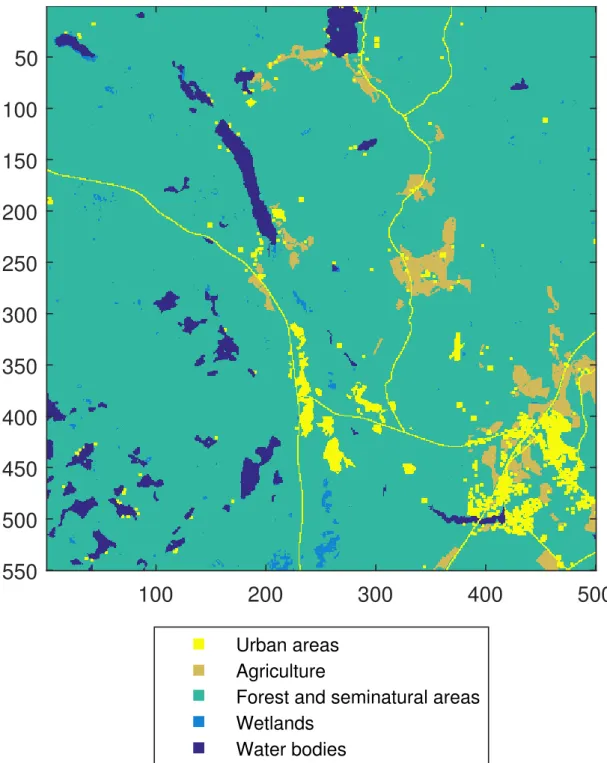
The CORINE land cover classes fall into five main categories, or level 1 classes: 1) artificial surfaces, 2) agricultural areas, 3) forests and semi-natural areas, 4) wetlands, and 5) water bodies. There are two additional levels of information common to all the CORINE participants, and additionally in Finland there are more accurate national 4th level classes available [3]. The classes present in the data are presented in the table 2.1, where the first number corresponds to the level 1 category, and the second number is a here defined value for the level 4 class information. It does not follow the CORINE numbering conventions, but is more intuitive in the classification framework. The CORINE level 1 classes are shown in a map in figure 2.4. The level 1 information is nationally 93 % accurate [3].

(10)

1.1 Continuous Urban 2.20 Agriculture 3.32 Very Sparse Forest 1.2 Discontinuous

Ur-ban

2.21 Agro-forestry 3.33 SparseForest/Mineral 1.3 Commercial 3.22 Broad-leaved

for-est/Mineral

3.34 SparseForest/Peat 1.4 Industrial 3.23 Broad-leaved

for-est/Peat

3.35 SparseForest/Rock 1.5 Traffic 3.24 Coniferous/Mineral 3.38 Bare rock

1.8 Mineral extraction sites

3.25 Coniferous/Peat 4.40 Inland marshes (land)

1.12 Summer cottages 3.26 Coniferous/Rock 4.41 Inland marshes (water)

1.13 Sport and leisure 3.27 Mixed/Mineral 4.42 Peatbogs

2.16 Fields 3.28 Mixed/Peat 5.46 Rivers

2.19 Pastures 3.29 Mixed/Rock 5.47 Lakes

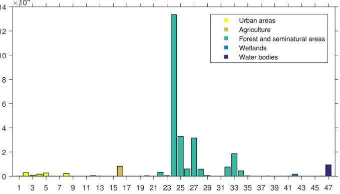
Table 2.1: The CORINE land cover classes present in the data. The first number in the class label identifies the level 1 CORINE category: 1) Urban areas, 2) Agricultural areas, 3) Forests and seminatural areas, 4) Wetlands and 5) Water bodies. The second number is a here introduced national level 4 category indentifier that does not follow the CORINE numbering conventions. 1 3 5 7 9 11 13 15 17 19 21 23 25 27 29 31 33 35 37 39 41 43 45 47 ×104 0 2 4 6 8 10 12 14 Urban areas Agriculture

Forest and seminatural areas Wetlands

Water bodies

Figure 2.2: The amounts of representatives in each class of the satellite data. The col-oring is based on the superclasses defined in table 2.1. The highest bar corresponds to coniferous/mineral forest.

(11)

Figure 2.3: The reference map of the Hyytiälä forestry station surroundings where the satellite data is obtained.

(12)

100

200

300

400

500

50

100

150

200

250

300

350

400

450

500

550

Urban areas Agriculture

Forest and seminatural areas Wetlands

Water bodies

(13)

2.2 Clustering

Clustering is a problem where the goal is to divide the data into similar groups. There are many definitions for the similarity in the clustering, and many algorithms with different assumptions and goals to perform the partitioning. Clustering is an unsupervised machine learning problem as no additional information to the data itself is assumed to be known, such as class labels. However to obtain results many of the methods make some other assumptions of the data, such that the data points are distributed according to some scheme, or that there is a certain amount of clusters to be found.

In this work two methods of clustering, Gaussian mixture models and a variant of this, k-means, are considered.

2.2.1 Gaussian mixture model

As the name suggests, mixture models model the situation when there are multiple prob-ability distributions that are sampled. It is a statistical generative model meaning that it describes how to obtain the samples. The sampling from a mixture is done by first randomly choosing one of the distributions belonging to it and then drawing a sample from that distribution. Mixture models can be used to model clustering, since the cluster can be thought to consisting of realizations of some distribution.

In Gaussian mixture models the distributions are assumed to be Gaussian, that is the j:th distribution has a probability density function

g(x;µj, Cj) = 1 p (2π)M_det(_C j) exp −1 2(x−µj) T_C−1 j (x−µj) where x ∈ _RM_, _µ

j ∈ RM is the mean and Cj ∈ RM×M is the covariance matrix. Each

of the distributions has a sampling probability πj which gives the probability of choosing

the said distribution when a sample is generated. It holds that

K X

j=1

πj = 1.

The probability density for the whole mixture distribution of K Gaussian components is

p(x, θ) = K X

j=1

πjg(x;µj, Cj),

(14)

The goal in mixture model clustering is to obtain the distribution parameters -sampling probabilities πj, means µj and covariance matrices Cj- that give the best likelihood for

the observed data. An often used method for maximizing the likelihood is Expectation Maximization (EM) algorithm.

The EM algorithm is given some initial conditions and the amount of clusters sought. It then repeats two steps, and M-steps for ’Expectation’ and ’Maximization’. In E-step it computes for each observed data point the probabilities of it belonging to the clusters. In M-step it calculates the new estimates that maximize the likelihood for the parameters based on the probabilities calculated in the E-step. These steps are repeated until convergence so that there is no change in the parameters or the change is very small. As the likelihood is guaranteed to increase in every step [12], the algorithm is also guaranteed to converge. However the convergence may not be to the optimal maximum, but rather to a local one. Indeed, the choosing of the initial conditions has a strong impact for the performance of the algorithm and it is often good to run it multiple times if there is not good information available for the set up. The following discussion follows [12, 13, 5].

If one assumes that the draws from the mixture model are independent, the likelihood function for unknown parameters θ and known data matrix X containing N data points

xn is Λ(X, θ) = N Y n=1 p(xn, θ) = N Y n=1 K X j=1 πjg(xn;µj, Cj)

Now the clustering problem can be formulated as maximization problem:

ˆ

θ = arg max

θ Λ(X, θ)

From the computational point of view it is often better to use logarithmic likelihood function, λ(X, θ) = N X n=1 log K X j=1 πjg(xn;µj, Cj),

instead of the likelihood function as the multiplications are transformed to summations. The likelihood maximization problem is equivalent to the maximization of logarithmic likelihood, so

ˆ

θ= arg max

(15)

In E-step the goal is to estimate the probability of a point given that it is drawn from the kth mixture, that is the probability _P(k|xn), k = 1, ..., K. With the definition of

conditional probability, that is with equation

P(A|B) = P(A∩B) P(B) ,

one can easily see that the said probability can be calculated as

P(k|xn) =

πkg(xn;µk, Ck) PK

j=1πjg(xn;µj, Cj) .

In the M-step the parameters µ(_ki), π(_ki) and C_k(i) are updated to µ(_ki+1), π(_ki+1) and C_k(i+1) so, that the logarithmic likelihoodλ(X, θ) is maximized. Here the upper index in brackets denotes the number of iteration. The parameters are calculated by evaluating the derivative of the function at zero. This yields new estimates

These steps give the algorithm 1. MATLAB’s functions are used in numerical calcu-lations.

2.2.2 K-Means

K-means is an unsupervised machine learning method for clustering. It is a special case of Gaussian mixture models, where covariance of the clusters is not considered, only the mean. The algorithm aims to find a good way of clustering the data by minimizing the sum of squared errors

k X i=1 X x∈Ci kx−cik2,

where Ci is the set of all the data points xfor which the cluster centroid ci is the closest.

As in the more general case, the algorithm is not guaranteed to converge to the global minimum, only to a local minimum.

(16)

Algorithm 1 Expectation Maximization for Gaussian mixture model

1: Estimate π(1)_k , µ(1)_k and C_k(1) for all K clusters.

2: repeat 3: E-Step:

4: for each object xn ∈X and cluster k ∈K do 5: _P(i)(k|xn) = π_k(i)g(xn;µ (i) k , C (i) k ) PK j=1π (i) j g(xn;µ (i) j , C (i) j ) 6: end for 7: M-Step:

8: for each cluster k ∈K do

13: until parameters πk, µk and Ck don’t change

Algorithm 2 k-means

1: repeat

2: for each data point x∈X do

3: assign xto the closest centroid

4: end for

5: for each cluster Ci ⊂X do

6: calculate the new centroid by taking the mean of datapoints x∈Ci 7: end for

(17)

As the algorithm isn’t guaranteed to converge to global minimum, the performance is strongly related to the starting conditions, i.e the centroids. The centroids can be guessed if there is reason to believe some particular clustering is the most likely. Also random initialization is often used, especially when computation isn’t so heavy that the clustering can not be repeated few times to ensure good results.

K-means can be varied based on the distance metric it uses. It can be for exam-ple (squared) euclidean, L1 or city block distance, correlation, or cosine measure. For numerical implementation we will use MATLAB’s kmeans-function.

2.3 Support Vector Machines

Support vector machine (SVM) is a supervised machine learning classifier. Unlike previ-ously introduced clustering methods, it utilizes the known class labels of the data. Based on given data and labels it searches for optimal separating hyperplane for the classifica-tion. The idea behind support vector machines is, that the data is mapped to some space where it is linearly separable and thus classification would be easier. However SVM:s work even for data that is not fully linearly separable even in the feature space. These properties make support vector machines very powerful classification tools. The following discussion of SVMs is based on [4, 5, 6, 7, 8, 9].

Support vector machines can be used directly in two-class classification. In the follow-ing we introduce support vector machines when data is assumed to be linearly separable and when it is not, and tell how the multiclass classification problem can be solved with the two-class classifiers.

For numerical implementation of support vector machines, we use MATLAB and its existing functions.

2.3.1 Hard-margin Support Vector Machine

Hard-margin support vector machines use the assumption that the data classified is linearly separable in the original m-dimensional input space, or alternatively in the l -dimensional feature space it is mapped to. As SVM is a supervised machine learning method, it is assumed that for all the training inputs xi there is the associated class label yi ∈ {−1,1} available.

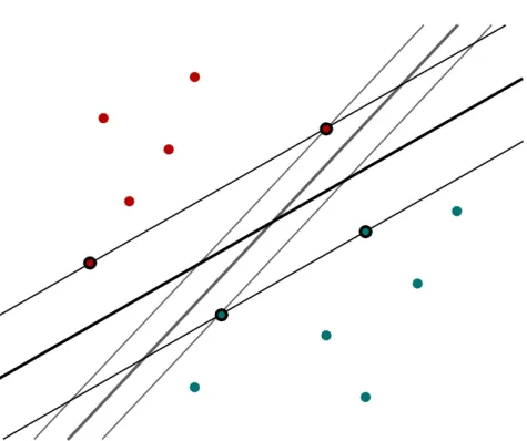
Figure 2.5 illustrates the idea behind support vector machines in two dimensions. Based on the input data and the classes, the goal of the SVM is to find an optimal separating hyperplane.

(18)

Figure 2.5: Illustration of the idea behind support vector machines in two dimensions. The SVM searches for the opptimal separating hyperplane with maximal margin, in the figure the thick black line. The data points marked with black circles are the support vectors.

linear separation, the decision function for classification is (2.1) D(xi) = wTφ(xi) +b,

where b is a bias term and w is an l-dimensional vector. Now the problem is to find the unknowns wandb for the optimal separating hyperplane, that is the hyperplane that has the widest distance between itself and the two nearest data samples. If the parameters w

and b are known, the classification of input vector xi is

xi ∈ (

class 1, if D(xi)>0

class -1, if D(xi)<0.

In the case D(xi) = 0, xi is not classifiable. However, it is assumed that the data is

linearly separable and so that is not possible. Indeed by suitable scaling of w and b in the above formula one can consider the cases greater or equal, or less or equal than one to control the separability. This scaling is done purely for ease of notation and doesn’t affect the classification.

(19)

The distance between the parallel line D(x) = 1 or D(x) = −1 and the separat-ing hyperplane is |D(x)|/kwk = 1/kwk. Now the optimal separating hyperplane which maximizes margin is obtained from the minimization problem

Minimize Q(w, b) = 1 2kwk

2

subject to yi(wTφ(xi) +b)≥1

Here minimizing kwk2 _{maximizes the margin} ₁_/_k_w_k _{of the hyperplane. The constant} 1 2 doesn’t change the optimization problem and is added purely to make it obey a standard form.

In solving this kind of constrained optimization problems a standard solution is to use Lagrangian multipliers. The method combines the constraint function with the original function to optimize. The optimization of the resulting function is equal to the original problem. A Lagrangian or Lagrangian function for the SVM optimization problem is

(2.2) L(w, b, α) = 1 2w T_w₋ M X i=1 αi yi(wTφ(xi) +b)−1 ,

whereα= (α1, ..., αM)T containing the nonnegative Lagrangian multipliers. The solution

for the optimization problem can be found among points where the partial derivatives of L are zero. This is addressed in the following theorem, which will not be proven here. Theorem 2.3. The global solution for the above quadratic programming problem 2.2 exists only if and only if the Karush-Kuhn-Tucker (KKT) conditions

∂L(w, b, α) ∂w =0 ∂L(w, b, α) ∂b =0 αi yi(wtφ(xi) +b)−1 = 0 for i= 1, ..., k αi ≥0 for i= 1, ..., k

are satisfied. The solution (w∗, b∗, α∗) that satisfies these conditions is the optimal solu-tion.

Often only the latter two conditions are called KKT conditions as the first two are just the extrema of the Lagrangian.

It is good to notice that not all of the training data have influence on the optimal separating hyperplane. The data instance that has the influence is called a support vector

(20)

and they are the data for which αi 6= 0 and thus (yi(wtφ(xi) +b)−1) = 0. See the

two-dimensional example from figure 2.5. Let us denote the set of the support vectors by S.

From the first two conditions of theorem 2.3 one can deduce that

w= M X i=1 αiyiφ(xi) (2.4) and M X i=1 αiyi = 0. (2.5)

Now substituting these and the last KKT condition into 2.2, the dual problem with constraints is obtained. Maximize Q(α) = M X i=1 αi − 1 2 M X i,j=1 αiαjyiyjφ(xi)Tφ(xj) subject to M X i=1 yiαi = 0, αi ≥0 fori= 1, ..., M

This dual problem is simpler than the original Lagrangian problem. It does not have

worb, but involves only the Lagrangian multipiers and the training data. The solution is still equivalent to the original one. The maximization arises from the negative quadratic term.

Kernel trick

The dot product φ(xi)Tφ(xj) in the l-dimensional feature space can be quite costly in

numerical calculations, especially whenlis much larger than the original dimensionalitym. There is however a solution around this problem that allows one to even make calculations in infinite dimensional feature space. The kernel trick means using kernel functions in calculations instead of the vector products.

Kernel functions are equivalent to the inner product in thel-dimensional feature space, that is

K(xi,xj) =φ(xi)Tφ(xj).

However one does not need to know the exact mapping φ, as long as the kernels fulfil Mercer’s theorem below. It ensures that the kernel functions can always be written as dot products of two input vectors in some high-dimensional space. Here the main idea behind the kernel trick is briefly introduced without proving it. See for example [10] for further reference.

(21)

In the theory of SVMs the reproducing kernel Hilbert spaces (RKHS) are important as they are the feature spaces the data is mapped to. The details are not gone through here, but the theory gives the justification of using kernels instead or the dot products of feature space. The following definition and theorem briefly summarize the results.

Definition 2.6. Symmetric functionK is positive semidefinite, if for all functions f 6= 0, f ∈L2, that is for all functions satisfying

R

f2₍_x₎_{dx <}_∞ _{it holds that}

Z Z

f(x)K(x, x0)f(x0)dxdx0 ≥0.

The definition is a generalization of positive semidefiniteness for matrices, here written again for comparison.

Definition 2.7. A M-by-M matrix K is called positive semidefinite, if for all arbitrary

hM = (h1, ..., hM)T, holds

hT_MKhM ≥0.

This is equivalent to all the eigenvalues of the matrix K being nonnegative.

The following theorem gives the justification of using kernels in support vector ma-chines.

Theorem 2.8. (Mercer’s theorem) Kernel function K can be written as

K(x,x0) =φ(xi)Tφ(x) if and only if it is positive semidefinite.

The condition for the kernel to be positive definite is often calledMercer’s condition. Based on the above theorem a positive definite kernel K(x,x0) can be used in the classification instead of φ(xi)Tφ(x). The maximization dual problem can be written with

kernels as Maximize Q(α) = M X i=1 αi− 1 2 M X i,j=1 αiαjyiyjK(xi,xj) subject to M X i=1 yiαi = 0, 0≤αi fori= 1, ..., M.

To conclude, with 2.4 the decision function 2.1 can be written D(x) =X i∈S αiyiφ(xi)Tφ(x) +b =X i∈S αiyiK(xi,x) +b

(22)

and

b =yj − X

i∈S

αiyiK(xi,xj).

The two classes are given by negative and positive values of D(x).

2.3.2 Soft-margin Support Vector Machine

Previous hard-margin support vector machines assume that the data is linearly separable in the feature space that it is mapped to. Although this might often be case, it is not guaranteed. In practice often used variant is a soft-margin Support vector machine, where it is possible that the data is not linearly separable but misclassifications are penalized.

For this goal, slack variables ξi ≥ 0 are introduced. They are zero when the

corre-sponding data point lies on the margin or behind it in the correct class area. When the data point is on the right side of the border but inside the margin area, the slack variables have values 0 ≤ ξi ≤ 1. When they are on the wrong side of the border, they obtain

values ξi ≥1. Now our constraints get form

yi(wTφ(xi) +b)≥1−ξi.

As we want to minimize the misclassifications, we also want to minimize the sum of the slack variables. Now the minimization problem is

Minimize Qsof t(w, b,ξ) = 1 2kwk 2 +C M X i=1 ξi subject to yi(wTφ(xi) +b)≥1−ξi, ξi ≥0,

where the term CPM

i=1ξi penalizes the wrong classifications and C is a parameter for determining the trade-off between maximization of the margin and minimization of the training error.

As in the case of hard-margin support vector machine, the minimization problem is solved by introducing nonnegative Lagrangian multipliers and the KKT conditions. One obtains a similar maximization problem using kernels,

Maximize Q(α) = M X i=1 αi− 1 2 M X i,j=1 αiαjyiyjK(xi,xj) subject to M X i=1 yiαi = 0, 0≤αi ≤C fori= 1, ..., M,

where the only difference is that αi values have to be less than equal to the trade-off

parameter C. The decision function is the same as with hard-margin support vector machine.

(23)

Solving the quadratic optimization problem in SVM

The most common algorithm for solving the quadratic optimization problem arising from SVM theory is Sequential Minimal Optimization (SMO) [11].

The algorithm breaks the optimization problem into smaller ones by searching through the feasible region to optimize and considering only two of the αi values at the time. The

other parameters are considered fixed. The αi values for optimization are chosen with

some heuristic.

In this study we use MATLAB’s functions for support vector machine classification. The default solver MATLAB uses is SMO.

2.3.3 Kernel functions for Support Vector Machines

Right choice of a kernel for classification is very important for the performance of SVM. There are multiple different kernels that are good at classifying data with different kind of features, here we present the most common ones.

Definition 2.9. Polynomial kernel with degree d∈_N is defined as K(x,x0) = (xTx0 + 1)d.

Kernel K(x,x0) = (xT_x0₎d_. _{can also be used, but it will not include all terms whose}

degree is lower than d so the first option might be better as it is more flexible. Theorem 2.10. Polynomial kernel fulfils the Mercer’s condition.

Proof. Calculating the kernel yields a summation.

K(x,x0) = (xTx0+ 1)d= (x1x01+...+xmx0m+ 1) d_{= (}_x

mx0m)

d₊_..._{+ 1}

Now φ(x) is a vector consisting of squared roots of the elements in the sum. This way φ(x)Tφ(x0) will equalK(x,x0).

If the data is linearly separable, the kernel used can belinear, so that K(x,x0) =xTx0.

This is a special case of a polynomial kernel.

Theorem 2.11. A kernel K(x,x0) =a when a≥0 is positive semidefinite.

Proof. Let φ(x) = (√a, ...,√a)T. Now for every length of φ it holds that K(x,x0) =

(24)

Theorem 2.12. Product of two semidefinite kernels K(x,x0) = K1(x,x0)K2(x,x0) is a

semidefinite kernel.

Proof. For a positive semidefinite matrix A it holds that A=FT_F_{, so we can write that} aij =fiTfj, wherefk is the kth column vector ofF.

Now for any h1, ...hm when B is also a positive semidefinite kernel, M X i,j=1 hihjfiTfjbij = M X i,j=1 (hifi)T(hjfj)bij ≥0

and thus the K(x,x0) is a positive semidefinite kernel.

Definition 2.13. Radial basis function (RBF) kernel or Gaussian kernel is defined by (2.14) K(x,x0) = e−γkx−x0k2,

where γ is parameter for radius.

Theorem 2.15. RBF kernel fulfils the Mercer’s condition. Proof. One can write

K(x,x0) = e−γkx−x0k2 =e−γkxk2e−γkx0k2e2γxTx0.

Here the first two exponentials are constants ≥0, and the third one can be represented as series expansion e2γxTx0 = 1 + 2γxTx0+(2γx T_x0₎2 2! + (2γxT_x0₎3 3! +...

which is an infinite dimensional polynomial. Thus from previous theorems we know that as a product of positive semidefinite kernels the RBF kernel is a positive semidefinite kernel.

In the case of RBF kernel the support vectors are the centres of the radial basis functions. RBF kernel is not very robust to outliers.

2.3.4 Multiclass Support Vector Machine Classification

Support vector machines can classify data into only two classes. Multiclass classification is possible with those, but it requires building multiple two-class classifiers. There are many ways of implementing the multiclass classification. In this study it is implemented in two different ways.

(25)

As support vector machines search for a division of the data into two different cate-gories, the multiclass implementations quite naturally want to find divisions of one class from the rest of the data. One can thus build as many classifiers of that kind as there are classes one wants to distinguish. Then one can use these classifiers for the data to be classified simultaneously. However, this kind of one-against-all approach can result to unclassified data instances or even instances that seem to belong to multiple data classes. This problem can be addressed with further classification methods, one of which is introduced below.

One can avoid these non-classifiable regions of the previous implementation by building support vector machines which work in succession. This means that the first SVM is build to classify one class from the rest of the data, while the second classifier will classify the second class from the data of which there are no instances of the first class to be classified. The last classifier will search for the optimal separation between two classes. In this implementation one needs to only build k−1 SVM classifiers for k data classes, in contrary to the previous implementation with k SVM classifiers.

K-Nearest Neighbours for classifying unknowns after SVM

K-nearest neighbours (k-NN) is a supervised machine learning technique. The algorithm is given a value k, number of nearest neighbours to check, and based on the classes of those k nearest neighbours it decides into what class should the object belong to.

In this study the method is used after some previous classification is obtained with multiclass support vector machine. The idea is to patch the obtained classification and its blank areas (i.e. those objects that couldn’t be for some reason classified). Since all the objects have a fixed place on the two-dimensional map grid, the k-NN determines based on the classifications around an object what the object likely is. As the data is in the grid formation, not all of the possible k values make sense. Reasonable values include 4 and 8, both of which are used in this study.

As the map data is most likely to be the same as the immediate neighbours, the k-NN algorithm will be first run with k = 4. As all of the four nearest pixels are at the same distant from the unknown, they have equal weights in the decision making process. If some class has a clear majority, this class is assigned to the unknown data point. The class updates are done after the whole map has been searched through. The k-NN algorithm is run until there are no new updates to be made to the map. After that the process is repeated with k= 8. As it is known that the four nearest neighbours couldn’t decide the class, all 8 neighbours have the same weight in the decision. This is also repeated until convergence.

(26)

Algorithm 3 k-nearest neighbours

1: input k: number of neighbours to search, M: data class map

2: Initialize new map N =M 3: repeat

4: for each index m of the map M do

5: find k nearest neighbours of indexm

6: if Some class i has majority in the neighbours then

7: update map N to have class i atm

8: end if

9: end for

10: M =N

11: until M does not change

12: return M

Overfitting and Performance Analysis

Overfitting is a common problem in machine learning with many causes including bad parameters in classification and features of the data. In overfitting the classifier performs perfectly with the data it is trained with but simultaneously loses the ability to generalize correctly. If this happens then for a data instance to be classified correctly as the overfitted class it would need to be virtually identical to one of the training examples of that class. To notice and avoid overfitting the data used in building the SVM classifiers is divided into two parts: training and testing (or control) sets. After the training is over, it is easy to see if there was overfitting by comparing the performances of the classifier with training and testing data. If the training data performs very well but the testing data very badly there has been overfitting. Ideally, the both cases should yield equally good results.

Overfitting can be noticed and to some extent prevented by selecting representative data for classification and adjusting the parameters of the classifier. To avoid over- and underfitting, MATLAB’s ’auto’ option is used for the RBF kernel scale, or theγparameter in the equation 2.14. With this option MATLAB determines the parameter by random subsampling.

SVM is a supervised machine learning method, which means that one has access to the actual data classes. This gives tools for analyzing the results.

After building the classifier, its performance can be analyzed with test or control data, e.g. some data from the same data set that has not been used in training the classifier. Since this is a two-class classification problem, the classifications can be divided into four categories: true positives (TP), false positives (FP), true negatives (TN) and false negatives (FN), when the classes are positive and negative.

(27)

Positive precision is defined as

posit. precision = TP

TP+FP

and it tells how many values that are classified as positive are correct. Positive recall (or sensitivity)

posit. recall = TP

TP+FN

tells how many of the positive values were correctly classified as positive. Negative preci-sion and recall are similar to their positive counterparts; positive changes to negative and vice versa in the formulas. Overall accuracy is defined as

accuracy = TP+TN

TP+TN+FP+FN and tells the total accuracy of the classifier.

(28)

Chapter 3 Results

In this chapter we describe the results for classification in the cases of simulated data set and the real satellite data with the methods described in previous chapter. The satellite data has been preprocessed before calculations by subtracting the mean from every time series.

3.1 Results with simulated data

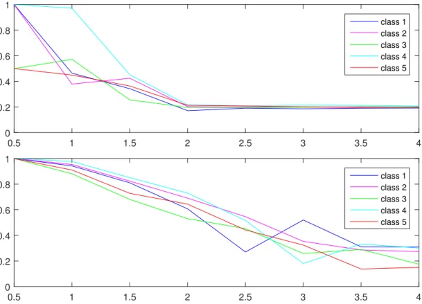
The classification of simulated data presented in section 2.1.1 was performed with Gaus-sian mixture models, k-means and support vector machines with different degrees of noise. Figure 3.1 illustrates the performance of Gaussian mixture models on the simulated data with no constraints on the covariance matrices and with diagonality constraint. The classification couldn’t be performed in the case where there is no noise since then the covariance matrices would be ill-conditioned.

Figure 3.2 shows the effect of noise level on the k-means classification.

The performance of support vector machines was tested by building five classifiers; each of them able to separate one class of everything else. In performance analysis the accuracies of each individual classifier are considered. The accuracies and positive recalls of the classifiers as a function of noise variance is shown in figure 3.3.

(29)

0.5 1 1.5 2 2.5 3 3.5 4 0 0.2 0.4 0.6 0.8 1 class 1 class 2 class 3 class 4 class 5 0.5 1 1.5 2 2.5 3 3.5 4 0 0.2 0.4 0.6 0.8 1 class 1 class 2 class 3 class 4 class 5

Figure 3.1: The results of Gaussian mixture model classification on simulated data from section 2.1.1. On x-axis the variance of the noise, and on they-axis the percentage of the class representatives in the cluster where the class has the most representatives. For the plot below the covariance matrices are constrained to be diagonal, while for the upper one there are no constraints.

0 0.5 1 1.5 2 2.5 3 3.5 4 0.2 0.4 0.6 0.8 1 class 1 class 2 class 3 class 4 class 5

Figure 3.2: The results of k-means classification on simulated data from section 2.1.1. On x-axis the variance of the noise, and on they-axis the percentige of the class representatives in the cluster where the class has the most representatives.

(30)

0 0.5 1 1.5 2 2.5 3 3.5 4 0.8 0.85 0.9 0.95 1 class 1 class 2 class 3 class 4 class 5 0 0.5 1 1.5 2 2.5 3 3.5 4 0 0.2 0.4 0.6 0.8 1 class 1 class 2 class 3 class 4 class 5

Figure 3.3: Above the individual accuracies of the support vector machines built for simu-lated data from section 2.1.1, below the positive recalls of those support vector machines. Both accuracy and recall are presented as a function of noise variance.

(31)

3.2 Results with satellite data

The section begins with simple visualization of the satellite data and proceeds to show the results of the two clustering methods. The last part of this section shows the results of support vector machine classification with the two approaches discussed in the section 2.3.4.

3.2.1 Visualization

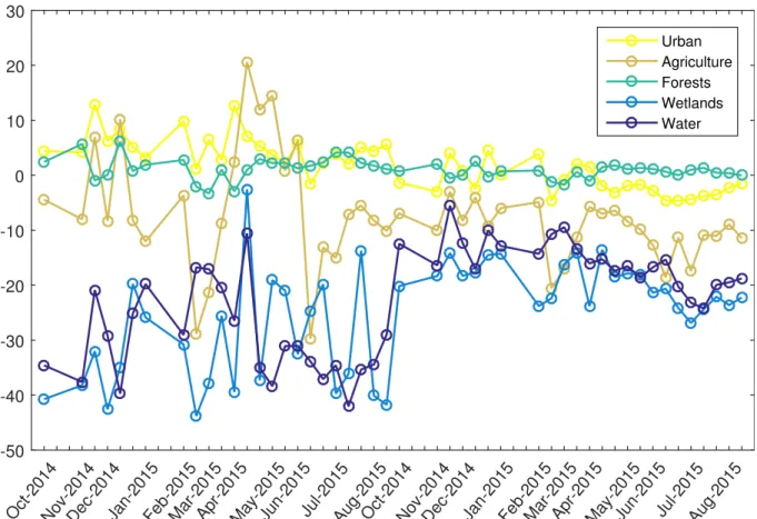
The mean series of the instances of each CORINE level 1 category is shown in figure 3.4. There seems to be some distinct features in all the classes, suggesting possibility of successful classification. Wetlands and waters are quite similar to each others, as are urban areas and forests. Agricultural areas stand out from both of them.

Oct-2014_Nov-2014_{Dec-2014Jan-2015}Feb-2015Mar-2015Apr-2015_May-2015Jun-2015Jul-2015Aug-2015Oct-2014Nov-2014Dec-2014Jan-2015Feb-2015Mar-2015Apr-2015_May-2015Jun-2015Jul-2015Aug-2015 -50 -40 -30 -20 -10 0 10 20 30 Urban Agriculture Forests Wetlands Water

Figure 3.4: Mean time series of each CORINE level 1 category. There are two different polarization images of each time instance.

(32)

3.2.2 Gaussian mixture model clustering

Gaussian mixture model clustering was performed with assumptions of 5, 8, 10, 12 and 30 clusters. When kwas 5 or 30, algorithm was initialized with the ground truth information of clusters, otherwise the initialization was random and the calculations were performed three times.

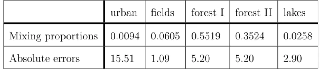
With k = 5 the algorithm was able to identify two clusters of mostly only lakes or fields, a cluster containing much urban areas but also some forest, and two very large clusters of forests. See figure 3.5 for histograms of the cluster compositions. The mixing proportions and absolute errors of the cluster means with respect to the superclass means are displayed in table 3.1. The resulting covariance matrices were not diagonal in any of the clusters.

When k grew larger few more features started to emerge. In addition to clusters containing fields, lakes and urban areas there was some variation in the forest clusters and their proportions. When k was greater than 12, the fields were divided into two or more clusters. When k was 30 there were some very small clusters consisting of members from only one class, but most of the clusters contained still members of many CORINE classes.

The clustering results were better when using full covariance matrices instead of diag-onal ones.

urban fields forest I forest II lakes Mixing proportions 0.0094 0.0605 0.5519 0.3524 0.0258 Absolute errors 15.51 1.09 5.20 5.20 2.90

Table 3.1: Mixing proportions of clusters from EM-algorithm whenk= 5, and the absolute errors of the cluster means to the closest superclass means. The clusters are in the same order as in figure 3.5.

3.2.3 K-Means clustering

K-means clustering was performed with values k ∈ {5,8,10,12,30}. As with Gaussian mixture models when k was 5 or 30 algorithm was initialized with the mean values based on the ground truth information of clusters, otherwise it used random initial centroids and the calculations were performed three times to lessen the impact of the initial choice. The clustering wasn’t as successful as with Gaussian mixture models, see figure 3.6.

(33)

Cluster 1:

Cluster 2:

Cluster 3:

Cluster 4:

Cluster 5:

Figure 3.5: Bar plots of the actual class lables of the time series instances in clusters found with Gaussian mixture models with k = 5. Notice the different scales on y-axis. The class numbering in x-axis follows the one in table 2.1 and the colour coding is based on the level 1 CORINE categories.

(34)

Cluster 1:

Cluster 2:

Cluster 3:

Cluster 4:

Cluster 5:

Figure 3.6: Bar plots of the actual class lables of the time series instances in clusters found with k-means algorithm when k = 5. Notice the different scales on y-axis. The class numbering in x-axis follows the one in table 2.1 and the colour coding is based on the level 1 CORINE categories.

(35)

Some things were the same with each k value. Majority of the lake instances formed always their own cluster with some additional time series instances from other classes. There was also always at least one very small cluster where the majority of instances were from urban category.

Fromk= 12on there was a cluster consisting almost only of field time series instances. Not all the field time series instances were there, as half of them were in a cluster consisting mainly of the forest time series instances.

No metric was better than the euclidean.

3.2.4 Support Vector Machine classification

The support vector machines for both approaches were trained with a fraction of the data available by trial and error. The training and testing data sets were selected to contain similar amounts of data from each category, tuned by trial and error. The parameter for kernel scale was determined automatically with MATLAB using random subsampling.

The results shown are obtained with RBF kernel, which performed better than poly-nomial.

The successive approach in SVM classification was performed with all possible super-class orderings. The accuracy of super-classification varied from 80.1% to 93.0%. To summarize the results shown in table 3.2 the earlier the forests were in the classification order the worse the performance. The best performances were obtained with the order: urban ar-eas, waters, agricultural arar-eas, wetlands and forests. Visualizations for some of the results are shown in figure 3.7.

The simultaneous classification with support vector machines was able to obtain 79.8 % accuracy on its own. Here 15.5 % of the time series instances were not classified at all. The accuracy measures of individual classifiers with the control data in the building stage are shown in table 3.3. The accuracies of the performance with the whole data set are shown in table 3.4. Some analysis on what time series were left uncertain in the classification is shown in figure 3.8 and table 3.5. Most of the data instances not classified are such that all classifiers labelled them as ’else’. No data instance was classified by the SVMs to belong into more than two superclass. The class label distribution of the instances not classified follows quite closely the distribution of the whole data set (figure 2.2).

The classification obtained from the SVM was further improved with k-nearest neigh-bours smoothing, which resulted in 92.7 % accuracy while only 0.7 % of the time series instances was left unknown. The accuracies are shown in table 3.6, while the illustration of the results on the reference map can be seen in figure 3.9.

(36)

order acc. order acc. order acc. order acc. order acc. 54321 85.8 45321 85.7 34521 80.1 24351 86.2 14325 91.4 54312 86.1 45312 86.0 34512 80.4 24315 86.3 14352 91.4 54231 89.8 45231 89.7 34251 80.1 24531 89.8 14235 92.8 54213 91.8 45213 91.7 34215 80.2 24513 91.8 14253 92.9 54123 92.7 45123 92.6 34125 80.5 24153 92.0 14523 92.9 54132 92.3 45132 92.2 34152 80.5 24135 92.0 14532 92.4 53421 84.5 43521 81.4 35421 80.1 23451 84.8 13425 91.0 53412 84.8 43512 81.7 35412 80.4 23415 84.9 13452 91.0 53241 84.4 43251 81.5 35241 80.1 23541 84.8 13245 91.0 53214 84.4 43215 81.5 35214 80.1 23514 84.8 13254 91.0 53124 84.8 43125 81.9 35124 80.4 23154 84.9 13524 90.9 53142 84.8 43152 81.9 35142 80.4 23145 84.9 13542 90.9 52341 88.9 42351 86.2 32541 80.1 25341 88.8 12345 92.8 52314 88.9 42315 86.3 32514 80.1 25314 88.8 12354 92.8 52431 89.8 42531 89.8 32451 80.1 25431 89.8 12435 92.8 52413 91.8 42513 91.8 32415 80.2 25413 91.7 12453 92.9 52143 92.0 42153 92.0 32145 80.2 25143 92.0 12543 93.0 52134 92.0 42135 92.0 32154 80.2 25134 92.0 12534 93.0 51324 92.1 41325 91.4 31524 80.5 21354 92.1 15324 92.1 51342 92.1 41352 91.4 31542 80.5 21345 92.1 15342 92.1 51234 92.9 41235 92.8 31254 80.6 21534 92.2 15234 93.0 51243 92.9 41253 92.8 31245 80.6 21543 92.2 15243 93.0 51423 92.8 41523 92.8 31425 80.6 21453 92.1 15423 92.9 51432 92.4 41532 92.3 31452 80.6 21435 92.1 15432 92.4

Table 3.2: Support vector machine classification results with ordered approach. The ordering is shown with superclass numbers from left to right, so for example 12345 means that urban areas were classified first, agricultural second etc. and everything not classified with the four classifiers is labeled as water. Darker background color implies higher accuracy.

(37)

50 100 150 200 250 300 350 400 450 500 50 100 150 200 250 300 350 400 450 500 550 50 100 150 200 250 300 350 400 450 500 50 100 150 200 250 300 350 400 450 500 550 50 100 150 200 250 300 350 400 450 500 50 100 150 200 250 300 350 400 450 500 550 50 100 150 200 250 300 350 400 450 500 50 100 150 200 250 300 350 400 450 500 550

Figure 3.7: Illustration of the classification results for ordered SVMs. The ground truth image is on the top left. Top right image illustrates the result from ordering 32514 with accuracy 80.1% , bottom left from 42315 with accuracy 86.3% and bottom right from 15243 with accuracy 93.0% (see table 3.2).

(38)

superclass positive precision positive recall negative precision negative recall accuracy Urban 0.658 0.206 0.867 0.980 0.856 Agricultural 0.849 0.555 0.927 0.983 0.920 Forests 0.798 0.837 0.661 0.600 0.755 Wetlands 0.917 0.336 0.958 0.998 0.958 Water 0.966 0.610 0.971 0.998 0.971

Table 3.3: The results of control data classification with support vector machines built to classify the CORINE superclasses in simultaneous multiclass classification. Negative class refers to the other four categories.

Superclass accuracy classified

Urban 0.552 5199

Agriculture 0.687 7510 Forest 0.967 211435 Wetlands 0.516 1154

Water 0.917 7023

Table 3.4: The accuracy of each superclass classification when support vector machines are used simultaneously to classify the whole data set. It is also shown in total how many time series instances were classified to each superclass.

(39)

1 3 5 7 9 11 13 15 17 19 21 23 25 27 29 31 33 35 37 39 41 43 45 47 ×104 0 0.5 1 1.5 2

Figure 3.8: Bar graph showing the amount of time series that were not classified in simultaneous SVM classification before applying k-nearest neighbours algorithm. In blue the amount of those time series instances that were not classified by any SVM and in cyan the ones that were classified in two superclasses. None were classified into more than two superclasses.

Superclass Agriculture Forests Wetlands Water

Urban 187 104 1 0

Agriculture 711 10 0

Forests 73 198

Wetlands 23

Table 3.5: Counts of how many times two classifiers classified same time series instances in simultaneous SVM classification approach.

Method correct wrong unknown

SVM 79.8 4.7 15.5

k-nn, k = 4 89.4 6.0 4.7 k-nn, k = 8 92.7 6.6 0.7

Table 3.6: The percentage of correct and wrong classifications and unknowns after simul-taneous SVM and k-nearest neighbour classifications. The k-nearest neighbour classifiers perform on the classification shown in the row above.

(40)

50 100 150 200 250 300 350 400 450 500 50 100 150 200 250 300 350 400 450 500 550 50 100 150 200 250 300 350 400 450 500 50 100 150 200 250 300 350 400 450 500 550 50 100 150 200 250 300 350 400 450 500 50 100 150 200 250 300 350 400 450 500 550 50 100 150 200 250 300 350 400 450 500 50 100 150 200 250 300 350 400 450 500 550

Figure 3.9: Illustration of the classification results with simultaneous SVM classification and k-nearest neighbour classification applied to the result. The ground truth image is in upper left corner, SVM result is in upper right corner, and on the bottom there are the results obtained with k-nearest neighbours smoothing: intermediate result with k= 4 on the left and the final result with also k = 8 on the right.

(41)

Chapter 4 Discussion

The goal of this work was to offer methods for developing automated analysis techniques for satellite data, focusing on automated recognition of different land cover types. This problem is be addressed with machine learning classification techniques. We used two dif-ferent approaches, namely supervised and unsupervised learning methods. These methods were tested with simulated data before applying them to the real satellite data. We were able to obtain as high as 93 % accuracy with the supervised machine learning approach. Of the data and the methods used in this work

The work in this study was done with data from Sentinel 1 satellite. The SAR images were preprocessed to have the time series instances to correspond to the pixels on the reference map. While the satellite images were taken with technique that isn’t bothered so much with the time of the day or obstructions such as cloud cover, one should still acknowledge that as it is real data there is likely to be anomalies. The effect of the possible anomalies is decreased as the amount of the data goes higher. The amount of data is somewhat a problem in this study as the different land cover types are very differently present in the data (see figure 2.2).

The time period of data acquisition goes from October 2014 to August 2015. As the time spans for almost an year one can assume that most of the yearly changes have been captured in the data set.

Some difficulties arise from the reference map interpretation of the time series data. Every pixel in the CORINE reference map corresponds to certain land cover superclass. In the nature however things are rarely nicely rectangular shaped or follow any other convenient formation. Thus some of the features might well fall into many pixels on the map and of which none contains it fully.

(42)

fea-ture of the data. Every pixel in the reference map from 2012 has some specific meaning. However, as the satellite images have been taken in 2014 and 2015, the CORINE infor-mation can be out of date to some extent. There can also be cases when the correct class of some pixel changes during the time when images have been taken and thus produces a time series which does not fully represent any of the classes. Also, the CORINE level 1 information for Finland land cover types used here for classification is only 93 % accurate in national level. This might in part create issues for classification.

Methods used in this study fall into two categories. Gaussian mixture models and their variant k-means are unsupervised machine learning techniques while Support vec-tor machines and k-nearest neighbours are supervised techniques. While the supervised techniques could initially be thought to be more effective in classification problems as they utilize the class labels of the data, the unsupervised machine learning techniques can still be used to find interesting structures from the data that might help in solving this problem.

Indeed from the point of view of the simulated data tests in the study the methods presented were very promising. Naturally when the noise was increased all the methods started to make mistakes, but all in all the results show that classification of some data is indeed possible with the methods presented in this study. The visualization of the superclass time series means shown in 3.4 further suggests this possibility.

Results with clustering methods

Although the clustering based approaches to study the satellite data were able to find some preferred structure from the data, there was much left to hope for. Unsurprisingly as Gaussian mixture model based clustering is able to identify more diverse clusters it performed better than k-means analysis, see figures 3.5 and 3.6. When considering the goal of finding the five level 1 CORINE classes from the data the clustering was first performed with k = 5. Both methods were able to identify most of the lakes into one cluster, but only Gaussian mixture models caught most of the CORINE class 16, fields, in a cluster. The fields were mostly in one cluster also in the case of k-means, but they were suppressed by forests there. It is good to note that both fields and lakes are a major representative of their level 1 CORINE class and can thought to be roughly equivalent to those in this study.

Both methods had formed additional two clusters of forests, and one cluster with urban areas. This cluster however was very small compared to the others. It was not very surprising that the wetland category hadn’t formed a cluster in either of the approaches as there were so few representatives. As in the case of fields with k-means, the wetlands were mostly present in only one cluster with majority of forest time series instances.

(43)

ground truth information. As discussed earlier, some pixels in the map might in reality correspond to more than one category while it is given only one.

The clusterings were performed with largerkvalues to see if there was some underlying structure present in the data that would make sense when considering the CORINE classes. Especially in the case of Gaussian mixture models some small features emerged, but no very good division along the CORINE categories. It was to be expected as the different amounts of different class representatives can heavily influence the clustering algorithms used. Most of the classes have too few representatives for finer classification to be meaningful.

Results with support vector machines

The classification results with both support vector machine implementations were very good with approximately same accuracies, see figure 4.1. Both implementations also had the same difficulties with the data, namely the classification of urban areas. Only major features were present in the final classification results while the smaller details such as roads and summer cottages were lost.

In the ordered approach to the classification the order had very strong effect to accu-racy; it varied from 80.1 % to 93.0 %. The common feature in the worse classifications is that in each of them the forests were classified before urban areas. In practice this means that when training the classifier for forests, the urban areas are included in training data, but the same does not hold for the classifier for urban areas. This results into a lot of actual forest being classified as urban areas (figure 3.7). As already seen from the data visualization in the section 3.2.1, the time series from urban and forestry areas resemble each other quite strongly. Indeed in Finland the urban areas tend to have quite much vegetation, a lot of which is also strongly present in roadsides. It is no wonder that these two categories would thus be difficult to separate in the analysis. Some urban areas were also mixed with agricultural ones.

The wetlands were another CORINE level 1 category that was difficult to classify with both approaches due to the small sample size of this class. Many of the smaller features were lost, but both methods quite correctly identified the wetlands at the southernmost area although the border line differed from the correct one.

The simultaneous approach in support vector machine classification smoothed with k-nearest neighbours yielded approximately the same accuracy as the ordered approach. The error was slightly smaller, but due to small amount of uncertainty left in classification the overall accuracy was slightly smaller.

When considering the results with the simultaneous approach in support vector ma-chine classification, the areas left unknown are very similarly distributed as the ones classified incorrectly in the worst scenarios of ordered classification. The result is not

(44)

sur-50 100 150 200 250 300 350 400 450 500 50 100 150 200 250 300 350 400 450 500 550 50 100 150 200 250 300 350 400 450 500 50 100 150 200 250 300 350 400 450 500 550

Figure 4.1: Comparison of the best results of different multiclass classification approaches with support vector machines. On the left is the best result from sequential SVM classi-fication approach, while on the right side is the result from simultaneous SVM approach with k-nearest neighbour filling applied to it. For the image on left the misclassification rate is 7%, while on the right it is 6.6% with 0.7 % of the class labels remaining unknown. prising when considering how the classifiers work in different approaches. The time series instances not classified are distributed among the different categories almost identically to the whole distribution, see figures 2.2 and 3.8.

There were not many conflicts among the different classifiers when considering the simultaneous approach, meaning that only few time series instances were tried to classify into two different categories. Most conflict was with agricultural and forest time series instances, see table 3.5. It is likely that the conflicts here arise from the pixelization of the map; for example it is likely that when classifiers for forest areas and waters are trying to classify the same time series instance, it corresponds to water bank like area. These instances are likely to have features from both of the categories they are tried to classify into.

The parameters and especially the data used in training the support vector machines affect a lot on the classification performance. As there was no specific definition what would be a good result or what parts of the classification are the most important we tuned the machines by trial and error and chose the ones giving good general results. It would

(45)

be possible to tune the classification more according to specific needs of some application. Future considerations

Overall the techniques worked quite as one would expect when consulting the visualization of the superclass time series means (3.4). Agricultural areas, waters and wetlands stand out from forest and urban areas and were often possible to recognize. The latter two were the most difficult ones to distinguish with any of the techniques used. This is quite reasonable as urban areas in Finland tend to be quite green and have lot of trees and parks.

Due to the small amount of the data available, we restricted the study into the CORINE level 1 categories. However as the data was also quite unevenly distributed among the categories some of the five classes were represented by instances from a single level 4 category. It would be interesting to see how the level 1 classification could be per-formed with more balanced data, or also would it be possible to distinguish finer features from this kind of data so that one could classify the data into smaller categories. For this study however these goals were not possible to reach towards as the data was lacking in that sense.

The results of this study offer a good foundation of automated satellite data analysis. Although the ultimate goal is still far ahead, the study has shown that this is a reasonable goal. Next step would be large scale implementation and testing of this kind of classifi-cation. It would also be interesting how well the classification results generalize to other areas than Finland. Possibility of using other kinds of satellite data than SAR images could also be studied. One intriguing idea to try would be to see how the yearly variations affect this kind of classification problem. What kind of generalization should one do to make a model that is able to reasonably well classify data from a given time period. On the other hand when one has a reliable map at given time one would only somehow keep track on the changes occurring, so one problem could be how to detect these changes from the time series. It is very likely that these kind of changes are also occurring in the data of this study, but with this amount it is very difficult to study the changes.

(46)

Bibliography

[1] ESA: Sentinel-1 User Handbook, September 2013 (available at https://sentinel.esa.int/ )

[2] Y. K. Chan and V. C. Koo: An Introduction to Synthetic Aperture Radar (SAR), Progress In Electromagnetics Research B, Vol. 2, 27–60, 2008

[3] Finnish Environment Institute SYKE: Producing land cover and land use data in CORINE Land Cover 2012 project in Finland, final report (available at http://www.syke.fi)

[4] Pang-Ning Tan, Michael Steinbach and Vipin Kumar: Introduction to Data Mining, Pearson, 2006

[5] William H. Press, Saul A Teukolsky, William T. Vetterling, Brian P. Flannery: Nu-merical recepies, The Art of Scientific Computing, Third Edition, Cambridge Uni-versity Press, 2007

[6] Kevin P. Murphy: Machine Learning: A Probabilistic Perspective, MIT press, 2012 [7] Shiego Abe: Support Vector Machines for Pattern Classification, second edition,

Springer, 2005

[8] Hal Daumé III: From Zero to Reproducing Hilbert Spaces in Twelve Pages or Less, 2004

[9] Corinna Cortes and Vladimir Vapnik: Support-Vector Networks, Kluwer Academic publishers, 1995

[10] Ingo Steinwart and Andreas Christmann: Support Vector Machines, Springer, 2008 [11] John Platt: Fast Training of Support Vector Machines using Sequential Minimal

Op-timization, in Advances in Kernel Methods – Support Vector Learning, B. Scholkopf, C. Burges, A. Smola, eds., MIT Press (1998).

(47)

[12] Geoffery McLachlan and David Peel: Finite Mixture Models, Wiley, 2000

[13] Aapo Hyvärinen: Unsupervised Machine Learning Lecture notes, University of Helsinki, 2015

[14] John Shawe-Taylor and Nello Cristianini: Support Vector Machines and other kernel-based learning methods, Cambridge University Press, 2000

Automatic identification of land cover types from satellite data with machine learning techniques