Investigating Machine Learning Clustering Methods to Replicate the Human Idea of Structure to Documents

(1)

Investigating Machine Learning Clustering

Methods to Replicate the Human Idea of

Structure to Documents

Johannes Jansson, Victor Miller

(2)

Abstract

Anyone trying to maintain a set of text documents in an information retrieval system will run into problems keeping it relevant and up to date as the amount of data increases. This thesis investigates how a collection of documents can be clustered in a way that resembles how a human would organize it. It also assesses how dicult it is to implement this into an existing information retrieval system with current programming libraries, and in what practical ways this can be useful.

The text data in this project is represented by a TF-IDF model. A K-Means clustering algorithm generates one clustering, and a Support Vector Machine is trained with minimal user data to provide another clustering. These two are then evaluated and compared using a set of metrics. This project takes a practical approach to the problem, focusing on what can be implemented using existing programming libraries and what will actually work in a production environment. Software for visualizing the corpus and calculating similar documents, are implemented as well.

The supervised method SVM greatly surpasses the unsupervised method K-Means in being able to replicate the given ground truth, but both mod-els are in themselves useful. With a relatively simple understanding of machine learning, any company could set up a similar system. It does, however, take some deeper mathematical knowledge and ne tuning to get the most out of it and tailor it to the dataset.

(3)

Acknowledgements

We want to thank our supervisor Martin Lundin from Talkative Labs, who made this entire project possible. We also want to thank our client, who taught us that when in doubt, always do both. A special thanks to our academic supervisor Kalle Åström, who guided us through this process and always encouraged us. Finally, we want to thank our signicant others and families for putting up with us this year and proofreading the text.

(4)

1 Introduction

This section aims to describe the underlying problem this thesis is based on and the target of the thesis. It also denes a context by discussing what has been done before both in this project and in other papers related to the same problem. Finally, it provides a description of the structure of this report.

1.1 Background

Large organizations often produce and store a large amount of internal doc-uments for their employees. The reason for this may vary but the common denominator is that the company itself wants the employees to get the informa-tion in these documents. In small organizainforma-tions this is not as big of a problem since the amount of content is limited. But in larger organizations, the amount of content grows and it becomes a problem to nd the documents you need. How can a system be created where the end users nd the needle in the haystack?

Most systems used in larger companies for their internal communication are based on tools from a time when the amount of information was small enough to overlook. They require manual work from a human being in order to keep the data in check and up to date. Few systems have been able to transcend this, and therefore their qualities have decreased as their sizes have increased.

To overcome these issues a search tool was built. The aim was to make it simple to access and nd the information needed in a fashion that the users were familiar with. To further improve the usability of the system the decision to learn from the user's behavior and to cluster documents based on their content was made. In this way, the possibility to present close relationships between documents but also tailor the experience for each user would be enabled.

1.2 Aim of the thesis

The aim of this thesis is to help our customer's employees nd more relevant content. This will be done by investigating and implementing Machine Learning clustering methods into an existing information retrieval system. The emphasis in this report is on implementing and evaluating dierent approaches rather than performing a theoretical analysis or development of the used methods. This is done in order to create as much value for the customer as possible. The main questions the authors asked was Can we replicate the human idea of structure to documents using software? and How does an unsupervised K-Means clustering perform compared to supervised Support Vector Machine in answering that question?.

Problem formulation

• Can we replicate the human idea of structure to documents using software? • How well does unsupervised K-Means replicate human clustering? • How well does a Support Vector Machine replicate human classication?

(8)

1.3 Previous work

Talkative Labs1 _{were approached with the problems mentioned above. The}

client had loads of useful content and a large number of employees who needed access to it but was unable to connect the two. Several full-time employees were required simply to organize the documents but people were still struggling to nd what they were looking for. The system relied heavily on navigating folder structures and browsing topics to nd what you were looking for. There had to be a better way to provide the users with the content they need.

To solve their problem an API that could serve dierent front-end applica-tions with data was built. On top of the API, a graphical user interface (GUI) was created, that the end users would interact with. In the rst iteration the GUI consisted of only a search eld.

The foundation on which this project stands on is a REST API. The API serves as the backend for the service that was initially built. The API handles all operations such as uploading/downloading assets, processing assets through creating previews and extracting text from them. All text data and metadata about the assets uploaded to the API is stored in a Mongo database with an elastic search index on top. This turned out to be a powerful solution for full-text search and content delivery. This was the information retrieval system that was already in place when this project started.

1.4 Related work

The paper Clustering articles based on semantic similarity written by Wang and Koopman [15] describes a similar situation to the one in this project. The authors have a large dataset that they want to cluster, but they do not have proper training data. They decided to use the unsupervised methods K-Means and Louvain community detection, and found K-Means to be very suitable for their needs. The paper describes K-means as one of the simplest unsupervised learning algorithms that solves the well dened clustering problem It scales well to large number of samples and has been used across a large range of application areas [15, p. 6]. This encouraged the use of the same method in this project.

Page seven in the same paper contains an interesting discussion about K-Means and mentions the importance of trying dierent values of K to nd what amount of clusters a dataset naturally falls into. This approach was also used in this project in order to get to know the corpus better. In their paper they do not have any base truth at all for evaluation, so they construct one using the average silhouette method. They then use this to determine the optimal number of clusters in their K-Means clustering. Since the label data in this project is not as good as we thought it would be this approach was very interesting to read. What they lacked was a comparison to a supervised metric, so that was one of the goals of this project.

In the paper A Comparative Study on Dierent Types of Approaches to Bengali document Categorization [5] the authors investigate dierent super-vised classication algorithms on Bengali documents. They nd that an SVM with TF-IDF feature vectors performs better than any other approach used in the study. They note that this result is consistent with other studies that have been conducted.

(9)

In the paper [6] the authors compare four supervised algorithms (Support Vector Machine, Decision Tree, K Nearest Neighbours and Naive Bayes). They arrive at the conclusion that for large document sets the SVM classier is su-perior to the others. SVM also surpassed its competitors in computational eciency. They used the metrics precision, recall and F-measure to evaluate the results. It is also interesting that they ran some tests with fairly small training sets (under 250 samples per category). They nd that SVM is not as good as the others for a small number of training samples but quickly passes the others as the number of samples grow. This is something that could have been interesting to evaluate for us when looking at the playlist model in our case.

Another interesting paper is Using unsupervised clustering approach to train the Support Vector Machine for text classication [8]. The title is self-explanatory and was immediately deemed interesting for this project. It would have been interesting to see how the K-Means data works as training input into the Support Vector Machine, and how that compares to the labels as training material. An even more interesting approach may have been to combine the knowledge of labels with the output of K-Means. Rather than creating training data out of no data, K-Means could be used to improve training data of low quality and then be fed to a Support Vector Machine. That was however outside the scope and timeframe of this project.

(10)

2 Theory

This section aims to describe the theoretical concepts that this thesis is based on. It starts with something as unusual as a description of an entrepreneurial term, but one that had great impact on to execution of this project. It then describes the theoretical foundations for the dierent methods and concepts used within the project.

2.1 LEAN

Lean is a system for how to develop a successful small business that resembles the scholarly method [11]. It starts out with some ideas about how to design a product and create value for the customers. The essence of the system is to test these ideas as early as possible, to promote learning and informed decisions. The rst step is to dene metrics for success and designing tests. The tests should be designed to be cheap to perform and fast to implement. The project then moves on to creating an MVP a Minimum Viable Product. An MVP is the smallest, simplest, fastest and cheapest way to bring value to the customers. Then the project moves on to test the idea. The tests give feedback both on whether the idea corresponds to the customer's needs and on whether the project is progressing. If that is the case, persevere and ne tune. If that is not the case, pivot into another, more productive, direction.

The LEAN system, like many business systems, sounds obvious by itself but really shines when compared to how things usually are done. It is not uncommon to start with some research and then work for a long time to perfect the product. The fear of releasing an unshed product takes the overhand but at the cost of missed feedback from the customers. The problem is that it is very easy to stray o course, or fail to notice that the demand has changed. This could result in unpleasant surprises in the late stages of the project. With a lean approach, these surprises can be detected early on and the project can adapt to it.

The LEAN system versus more traditional development methods also resem-bles the relationship between working in an agile way versus the waterfall model in software engineering. In this thesis, the LEAN model has been adopted to best fulll the customer's needs.

2.2 Text operations in text analysis

The parameters used in the vectorizer was maximum and minimum document frequency, a maximum number of features, a list of stopwords and the n-gram range.

2.2.1 Stopwords

Some words do not really contribute anything to the meaning of the document or are so common that they do not help dierentiating documents. These words are not included as terms in the machine learning data model. They are called stopwords. The NLTK [2] contains a list of such stopwords for dierent

(11)

lan-guages. Examples are me, your, up, further and very2_{. The decision to add}

some words that are common in this specic corpus was also made. 2.2.2 Tokenization

Tokenization is the process of moving from a list of characters to a list of words, or tokens, also referred to as terms [7, p. 22]. The list of characters is split wherever a space or a non-word character is encountered. There are of course some special cases, such as aren't and co-education that has to be handled in a special manner [7, p. 24].

2.2.3 n-grams

Some words belong together. This goes for both hyphenated words, that might be split by the tokenization process mentioned above, and words that are actu-ally separated by a space. The most classic example is probably San Francisco, but other common patterns are names (John Doe) and some terms of art (ma-chine learning). Words that frequently appear together lose some meaning if they are split up. Therefore, words that occur together frequently are stored as a single term in the data model. A term with two words is a bi-gram, and a term with n words is an n-gram.

2.2.4 Stemming

Stemming (or lemmatization) is the process of removing or replacing parts of words, usually axes, so that two words with the same meaning end up in the same term. Stemming is performed by removing axes so that car, cars, car's and cars' all end up within the same term car. Lemmatization uses a lexicon and understanding of grammar, so that terms like be, am, are and is all end up within the term be [7, p. 32].

2.2.5 Ignoring common/uncommon words

The nal text operation used in this project is automatic removal of words that are extraordinarily common or uncommon in a document. This is done to clean up the TF-IDF matrix and to speed up the learning process. The TF-IDF vectorizer automatically discards any words above or below a given threshold when it creates the TF-IDF matrix. Since they would not aect the outcome much anyway they might as well be removed in order to speed up the process.

2.3 TF-IDF

The data model used for this machine learning project was the TF-IDF model, where each row represents a document and each column represents a term (or feature) of the corpus. The term can be either a word or an n-gram. Each value in this matrix represents how common a specic term is within a specic document. The TF-IDF matrix is calculated in three steps: the term frequency step, the inverse document frequency step, and the combination step.

2_{The complete list of 127 stopwords in NLTK can be found here: https://gist.github.}

(12)

The rst step is quite simple. In order to assign a weight for a term in a document we simply count the number of occurrences of that term in the specic document. This is dened as the term frequency tft,d [7, p. 117].

The second step is more interesting. The issue with term frequency is that it handles all words in the same manner. A word with high occurrence in a document will weigh more than a word with a low occurrence, even if that word is very common in the entire corpus. A more desirable outcome would be that words that are uncommon in the corpus but common in a document are assigned a greater weight.

That is exactly what inverse document frequency does. The inverse docu-ment frequency for a termidft is dened as

idft= log N

dft

, (1)

where N is the total number of documents in the collection and dft is the

doc-ument frequency, the number of docdoc-uments containing the termt.

In the end we store the TF-IDF value, dened as

tf-idft,d=tft,d×idft. (2)

The TF-IDF vectorizer performs this operation for a corpus of documents. In order to clean up the TF-IDF matrix it also takes some parameters dened in section 3.5.2. In this project a list of stopwords was used, as well as a maximum and minimum document frequency, a maximum number of features, and an n-gram limit.

2.4 K-Means

K-Means is a clustering method based on minimizing the distance between the documents of a cluster and its center point, its centroid [7, p. 360]. The most important property of a cluster in K-Means is the centroid. The centroidµ of

a clusterω is calculated as µ(ω) = 1 |ω| X x∈ω x. (3)

The goal of the K-Means clustering is to minimize the Euclidian distance be-tween the centroid and all items belonging to a cluster. This distance is mini-mized via the objective function Residual Sum of Squares:

RSSk= X x∈ωk |x−µ(ωk)|2_, ₍₄₎ RSS= K X k=1 RSSk. (5)

First, each item is randomly assigned to a cluster, and the centroids are calcu-lated. The algorithm then reassigns documents to belong to the cluster repre-sented by their closest centroid, and the centroids are recalculated. These two steps are repeated until the clustering is done.

The clustering is done when one of four things happen. One, the RSS value becomes smaller than a predened value (the clustering is good enough). Two,

(13)

the RSS value decreases more slowly than a predened value (what we're doing is not enough). Three, the clustering stops changing between iterations (there is nothing left to do). Four, the number of iterations becomes larger than a predened value (we do not have time to wait anymore).

There is no guarantee that the algorithm nds the global optimum, so it is usually executed several times with dierent initial conditions to improve the overall results.

2.5 Support Vector Machine

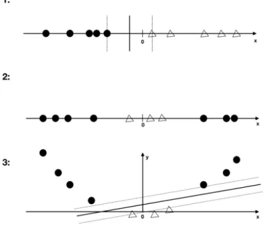
The idea behind using a Support Vector Machine (SVM) in this project is to train a system to recognize documents that would end up in the same folder if they were to be sorted by a human. The main principle of an SVM is to determine one or more separators in the feature room which best separates the classes (or folders, to use an analogy) [1, p. 194].

The simplest example of an SVM is a binary classier which separates two dierent classes with a hyperplane. If the training data is easy to separate this can easily be done with a linear approach. The optimization problem can be described as nding the plane with the largest margin to the support vectors, as seen in gure 1.

Figure 1: The main principle of an SVM illustrated. The target of the optimization problem is maximizing the margin between the support vectors.

If one wants to separate more than two classes the problem becomes more complex. The most common technique according to [7, p. 330] is to build a

(14)

one-versus-rest (ovr) classier that classies one class at a time against all the others.

All of the above applies to input data that is linearly separable, but in the general case for text classication the that is not the case [7, p. 327]. One way to solve this is the kernel trick. It's performed by mapping the input data to a higher dimensional space and then using the linear classier in that space.

Figure 2: The rst example is easy to linearly separate. The second one is more problematic. Using the kernel trick to map it into a higher dimensional space (case number 3) makes it possible

to separate them with a linear approach [7, p. 333]. 2.5.1 Kernel functions

scikit-learn supports four dierent kernel functions [13] out of the box. It also has a fth option to provide a custom kernel function. This makes it possible to test dierent kernel functions to nd the one that best separates the classes. The radial basis function is the default kernel function, and the linear kernel function the simplest one. The polynomial and the sigmoid kernel functions were also included in the model. The kernel functions are described in table 1.

(15)

Table 1: Mathematical denitions for the SVM kernel functions. RBF κ(x,x0) =e−γkx−x0k2 Linear κ(x,x0) =hx,x0i Polynomial κ(x,x0) = (γhx,x0i+r)d Sigmoid κ(x,x0) = (tanh(γhx,x0i+r))

2.6 Norms

2.6.1 Euclidian norm

The Euclidian norm is used in the K-Means clustering to determine the distance between documents and the centroid. It calculates the distance between the tips of two vectors. The Euclidian distance between two vectors is dened as

kx−yk= v u u t M X i=1 (xi−yi)2_, (6)

where x and y are vectors [7, p. 131]. The euclidian norm also goes by the name L2-norm.

2.6.2 Cosine norm

The cosine norm is used for visualizing data and for calculating document neigh-bors via document similarity. It calculates the angle between two vectors. In this project it was applied to feature vectors in the TF-IDF model to determine their similarity. The cosine similarity of two vectors is dened as

cosine similarity= x·y

kxkkyk, (7)

where x and y are vectors [7, p. 121]. The metric returns the angle between the two arrays independent from the length of the array. 1 for zero degree dierence, 0 for 90 degree dierence and −1 for 180 degree dierence. In the TF-IDF model, all feature vector components are positive, so the result of the cosine norm is bounded by 0and1. Two documents in the model are similar if the similarity is close to 1, and dissimilar if the similarity is close to 0.

2.7 Multidimensional Scaling

Moving from a set of coordinates to a table of distances is an easy mathemat-ical problem - just select a norm, calculate the pairwise distances and store it somewhere. The inverse problem, using distances to create a set of coordinates, is more complicated.

Multidimensional scaling (MDS) is a method for visualizing distance matri-ces. The goal of an MDS analysis is to nd a spatial conguration of objects when all that is known is some measure of their general (dis)similarity. [16, p.9].

(16)

There are two branches of MDS: metric and non-metric. The metric, simpler, version assumes all distances are actual euclidian distances. The nonmetric, more general, version makes no such assumption and is therefore more complex. The most common approach to nonmetric MDS is to dene some measurment of stress, that measures how much a given set of coordinates dier from the given distance matrix. The target for the MDS method is to minimize this stress.

In this project, the manifold package in scikit-learn was used to achieve a visualization of the clusterings. It uses the SMACOF algorithm, short for Scaling by Majorizing a Complicated Function [3, ch. 8]. SMACOF starts out with a random coordinate assignment. It then calculates a specic stress matrix for the assignment. In order to minimize the stress, the Guttman transform is performed on the coordinates X [3, p. 190]. For the reader interested in the

specics of the stress matrix, and the Guttman transform, reading chapter eight of the title Modern Multidimensional Scaling [3] is recommended. After the transform the stress is calculated again. If it satises a predetermined condition, or if it has reached the maximum number of iterations, then it terminates. If not, the transform is repeated. The process is described in gure 3.

Figure 3: An overview of the SMACOF algorithm. Source: page 192 of [3].

The purpose of MDS in this project was to provide a way to visualize the dataset and the clusterings. While TF-IDF is a great format for computers, the MDS is the peeking hole for us humans to understand what is going on.

2.8 Metrics

In order to evaluate the results of this project, a selection of information retrieval metrics was selected. Each of them require both the outcome of a clustering and a set of labels (a ground truth) to compare them to. These will be explained in this section of the report.

(17)

2.8.1 Purity

Purity is the rst evaluation metric for clusterings. When calculating purity each cluster is assigned the label that is most frequent in that cluster. The ac-curacy of the clustering is then calculated by counting the number of correctly assigned documents divided by the number of documents. Mathematically pu-rity is dened as purity(Ω,C) = 1 N X k max j |ωk∩cj|, (8)

where Ω ={ω1, ω2, ..., ωK} is the set of clusters and C={c1, c2, ..., cK} is the

set of labels used for evaluation [7, p. 356]. A number close to one represents an accurate clustering and a number close to zero represents a bad clustering. It is also important to note that a high purity is more easy to achieve when the number of clusters is high.

Purity is a metric that is very intuitive and easy to grasp. It also has the advantage that it can be calculated per cluster, not just per clustering. This provides accuracy for the analysis of the clusterings.

2.8.2 Entropy

The second metric used to evaluate clusterings is entropy. Entropy is a way to measure the amount of order or disorder in a system. A low entropy means that the clusters are well ordered and predictable, while a higher entropy means that the clustering is more chaotic. The entropy H of a clusterω is dened as

H(ω) =−X c∈C P(ωc) log₂P(ωc) =−X c∈C |ωc| nω log₂|ωc| nω (9) in [7, p. 99-100], with added maximum likelihood estimates of the probabilities. |ωc|is the number of documents classied ascin clusterω, andnωis the number

of documents in cluster ω. The total entropy of a clustering was then dened

as the weighted average of each cluster, calculated as

H(Ω) = X

ω∈Ω

H(ω)Nω

N , (10)

where Ω is the set of clusters{ω1, ω2,· · ·, ωk}, N is the total number of

doc-uments and Nω is the number of documents in cluster ω. Unlike all other

metrics, zero is a perfect score for this metric, and a higher value means that the clustering is less successful.

The entropy metric has the same two advantages as purity: it is intuitive3

and it can be calculated per cluster, not just per clustering. 2.8.3 True or false, positive or negative

In order to understand our next few metrics, a few terms need to be introduced. When comparing a computed clustering to a set of labels (or keys), four dif-ferent cases arise. When a document occurs in a cluster, and it should, it is a

(18)

true positive. If a document occurs in a cluster, and it should not, it is a false positive. Similarly if a document does not occur in a cluster and it should nott, it is a true negative. If a document does not occur in a cluster, but it should, it is a false negative. Table 2 summarizes this paragraph.

Table 2: True and false positives and negatives Relevant Non-relevant Retrieved true positives (tp) false positives (fp) Not retrieved false negatives (fn) true negatives (tn)

2.8.4 Precision and recall

The next two metrics are precision and recall. Precision is dened as the per-centage of the retrieved documents that are relevant, or true. Recall, on the other hand, is the percentage of the relevant, or true, documents that are re-trieved. Mathematically they are dened as

P= TP

TP+FP, (11)

R= TP

TP+FN. (12)

Intuitively precision ensures that the received results have a high relevancy, while recall makes sure the user is not missing out on anything important. Precision and recall are calculated for the SVM model in its cross validation phase, but is not calculated for the K-Means clustering.

2.8.5 F-score

The next metric is F-score. F-score combines the concepts of precision and recall using the weighted harmonic mean. This is dened as

Fβ=

1

α_P1 + (1−α)_R1, (13)

but with β2₌1−α

α this can be written more compactly as

Fβ=

(β2+ 1)PR

β2P₊R (14)

β ∈[0,∞]. In F-score the parameterβcan be chosen arbitrarily. A higher value

penalizes false negatives harder, a lower value penalizes false positives harder.

β = 1emphasizes precision and recall equally. Fβ= 1is a perfect score for this

metric, and a lower value means that the clustering is less successful.

F-score is calculated for the SVM model in its cross validation phase, but is not calculated for the K-Means clustering.

(19)

2.8.6 Homogeneity completeness and Vmeasure

The next set of metrics are homogeneity score (hs), completeness score (cs) and

Vmeasure score (vms). These three belong together, just like precision, recall

and F-score do. They were selected primarily because of their intuitive meaning, they really tell something about the properties of the clusterings. Homogeneity means that each cluster contains only members of a single class [12, p. 411]. Completeness means that all members of a given class are assigned to the same cluster [12, p. 411]. When creating a clustering it is quite easy to maximize one or the other of these two metrics, and one might prioritize one over the other in some cases. But a great clustering should seek to maximize both, so V measure score is dened as the harmonic mean of the homogeneity score and the completeness score. A high Vmeasure score is achieved by making a clustering which is high in both homogeneity and completeness, so the Vmeasure score may be considered a more broad or general metric for a clustering. All of the three metrics take values between one and zero, where one is the maximum score (an entirely homogeneous and/or fully complete clustering) and zero is the minimum score.

One drawback to this group of metrics is that they are not chance normalized, so one has to be careful when the number of clusters is large or the number of items is small. The Vmeasure score is equivalent to Normalized Mutual Information, which is another very common metric of a clustering.

Mathematically, these metrics are dened as

h= 1−H(C|K) H(C) , (15) c= 1−H(K|C) H(K) , (16) v= 2· h·c h+c, (17)

with the conditional entropy of classes C given cluster assignment K H(C|K) and the entropy of classesC H(C)dened as:

H(C|K) =− |C| X c=1 |K| X k=1 nc,k n ·log _nc,k nk , (18) H(C) =− |C| X c=1 nc n ·log nc n . (19) 2.8.7 Rand index

This metric is useful for understanding another metric in this project, even though it is not used in itself. Based on the terminology in section 2.8.3, the Rand index is dened as

RI= TP+TN

TP+FP+FN+TN. (20)

Intuitively the Rand index is a measurement on how many percent of the doc-uments that were clustered correctly. A Rand index of one is a perfect score, and lower values indicate a bad clustering.

(20)

2.8.8 Adjusted Rand score

The adjusted Rand score (ars) is based on the same principles as the Rand index,

but with two major dierences. The rst being that it ignores permutations. The actual names of the clusters do not matter, and it does not need a mapping between which of the generated clusters that should correspond to which of the ground truth clusters. The second being that it uses chance normalization. This means that the method projects a random clustering to the value zero by subtracting the expected valueE[RI], and then scales the values so that 1 is a perfect score and minus one is the worst achievable score.

The Rand indexRI can also be written as RI= a+b

Cnsamples

2

, (21)

whereais the number of pairs that are in the same set in both clusterings,bis

the number of pairs that are in dierent sets in both clusterings andCnsamples

2

is the number of possible pairs in the dataset. acorresponds to the concept of

true positives and the b corresponds to true negatives in section 2.8.3, but

does not actually use the label names of the clusters. Equation 21 is analogous to equation 20. The adjusted Rand indexARI of a clustering is then dened as

ARI= RI−E[RI]

max(RI)−E[RI], (22)

in order to perform the chance normalization. Since it considers both precision and recall it is considered a broad metric.

2.8.9 Fowlkes Mallows Score

Fowlkes Mallows score (f ms) is another broad metric that tries to consider

all aspects of a clustering. It is based on pairwise precision and recall. Mathe-matically it can be dened as

FMI= _p TP

(TP+FP)(TP+FN) (23) in [14, p. 6], borrowing notation from the previous section 2.8.3. A value close to one is an indication of a good clustering and a value close to zero of a bad one. The metric is chance normalized so that random label assignments have a Fowlkes Mallows score close to 0. It is also important to note that fms will always assume high values for very low numbers of clusters.

(21)

3 Method

This section aims to describe the execution of the project. It begins by describing the approach and explaining some obstacles that aected the choice of methods. It then goes on to describe the rst naive steps of the project and some remarks about the kinds of data that was available. The most important part is code implementation, which describes how the machine learning system is built and structured. Finally, it describes the architecture the project was executed on.

3.1 Approach

3.1.1 LEAN

A very important part of the approach has been the LEAN model. The primary target, or metric for success, was not a theoretical question. It was: how far can two engineering students go in creating a useful machine learning system? Since that was not clear at rst the decision to work in iterations was made, based on the customer's feedback. Build, measure, learn, repeat. Not read, think, do, done. For us this meant two things.

First, customer preference over our preference. The work was divided into small iterations that were presented to the customer. In between each iteration there was feedback and new requests that aected the direction and momentum of the project. This did turn out to be quite dierent from the method we were used to from the university, where most things are planned and have a structure. Lectures and readings cover material that is later required to solve the problem. Introduction, theory, method, results, discussion. In the corporate world result is king, discussions come before method, and theory is kept to a minimum.

Balancing customer demands and keeping track of the problem formulation has been challenging but also rewarding. With a more classic approach we would have ended up with a very dierent solution, but with a lot less knowledge.

Second, implementation over theory. This project is all about what could be done and maintained within the timeline and/or budget, and what results could be achieved. The customer always wants results.

These circumstances may be worth keeping in mind whilst reading this report and understanding the decisions made along the way. These were the internal factors but there were also some external factors that aected our decisions. They will be presented in the following section.

3.2 Challenges

The previous section outlined the benets of the chosen approach. This section will move on to some obstacles. Given below are four challenges that resulted in some road changes.

3.2.1 Developing in a live environment

The challenges of doing a project at a company, for a customer, has been very rewarding for us and the nal outcome of the project. Nevertheless, it also made the journey more dicult. Things have taken more time than we had envisioned. Likewise, regarding the programming; writing a script that runs on

(22)

your computer when you need it to is one thing, but integrating your code into a codebase that does not allow any downtime is a dierent thing. This has been challenging and fun, but has also slowed us down quite a bit. A lot of time was spent writing API:s and integrations that would not have been required if the project's only purpose was this report.

3.2.2 Corporate politics

Our greatest obstacle to overcome has been corporate politics. During the rst months of this project everything was running ne and we counted on an inow of users according to a prognosis. We therefore decided to focus on supervised machine learning systems: systems that collect and make sense of user data. Suddenly this changed, due to corporate politics, as it was decided that we would wait an additional month before adding users. We kept working on the supervised systems. The month quickly turned into two months and we were getting worried. Eventually, we realized that we could not rely on user data and had to change the direction of this project altogether and look for alternate data sources. The data source we ended up with is explained in section 3.4. 3.2.3 Search optimization

In the early stages of the project, a lot of time was spent on researching how to use machine learning to improve the search results of the service. This made sense as searching is the number one way for users to interact with the informa-tion platform. Unfortunately this turned out to be a dead end.

3.2.4 word2vec

As a rst step word2vec was used on the text of the entire dataset [1]. Raw text data was downloaded from the database and fed into the python implementation of Google's word2vec and training and clustering of the terms occurred. This provided insights on how the terms in the documents were related but did not directly help to understand the relationships between documents. The method was dropped in favor of other methods, more focused on documents.

3.3 Naive rst steps

With all these things in mind, how does one go about investigating machine learning methods that replicate the human idea of structure? Since the problem formulation did not imply a specic method the rst couple of weeks mainly consisted of experiments to gure out the road ahead and to get acquainted with the dierent available methods for machine learning.

3.3.1 TF-IDF demo

The rst step was constructing a TF-IDF matrix and a clustering with K-Means. This quickly became the primary method of clustering in this project. It also seved as an introduction to a lot of machine learning concepts and to scikit-learn [9]. The Python library scikit-scikit-learn is a popular collection of tools for machine learning.

(23)

A list of le hashes and all the text content of the les were loaded into the system. A number of operations were performed on the text. All non-text characters were replaced with spaces. Stopwords were removed using a corpus from Natural Language Toolkit [2]. Finally the text was tokenized and stemmed. This data was then loaded into TdfVectorizer, a feature extraction function from scikit-learn, that generated the TF-IDF matrix from the contents of all documents. The vectorizer also automatically ignored the most and least common words.

With the TF-IDF matrix in place, all pairwise distances were computed using the cosine norm. This data was used for visualizing the data. The clustering instead relied on scikit-learns K-Means tool that uses the TF-IDF matrix and number of clusters as inputs.

3.3.2 Cluster visualizer

Finally, the need for a way to visualize the documents and their feature vectors emerged. In order to get a visualization the scikit-learn tool MDS was used, short for Multi-dimensional Scaling, and the classic python tool Matplotlib [4]. MDS uses the cosine norm distance matrix and generated a 2D representation of all documents. These were plotted in matplotlib as a scatter plot with colors based on cluster.

These were the rst steps to probe the problem and get used to some machine learning methods and libraries. In order to make something truly useful, a better structure and method for evaluation was required.

3.4 The Data

As is always the case with machine learning solutions, the data is the most essential part. We will therefore elaborate what kind of data we had access to and how it was processed.

3.4.1 The corpus

The corpus consists of approximately 18400 pdf documents. They are internal guidelines, product specications, safety labels, slide-decks and reports written for the employees of the company. The scope of this project is only raw text extracted from the pdfs, not images or layouts.

3.4.2 The user data

The user data comes in two dierent forms. One, in the form of playlists and the other in the form of user anlytics, which will be explaind further on. Users, and admins, can create playlists containing one or several documents from the corpus. A playlist provides two pieces of information. Firstly, each document in the playlist is somehow related to the words in the title of the playlist. Secondly, each document in that playlist is somehow related to all of the other documents in the playlist.

The other form of user data comes from Segments4_{, a web user analytics}

tool. It was congured to track events such as The user performs a search and

(24)

The user navigates through the preview. This connected documents to each other, and documents to search queries. Since the information retrieval system had very few users none of this data could be used in this thesis.

3.4.3 URL data

The old system had a unique URL for each document. This URL was retrieved and stored in the data model and became the training data for this thesis.

The full URL:s were unique, so they would not work as training data. The solution to this was to only look at a certain level of the URL. Level = 0 only looked at the rst part of the URL, for example /Performance. Level = 1 looked at the rst two parts of the URL, for example /Performance/Lists. In this way, dierent sizes of clusters or classes could be generated by varying the level parameter. This was then used as training data for the supervised method, and as evaluation data for the metrics.

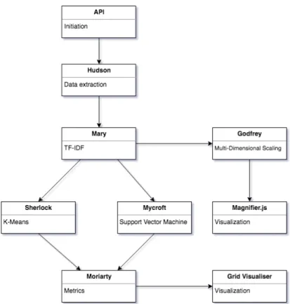
3.5 Code implementation

This section will explain the machine learning process based on the structure of the code. A short overview is presented below in list and diagram form (gure 4), each one is then described by a subsection. Each part of the implementation was named after a famous character from Sir Arthur Conan Doyle's legendary story Sherlock Holmes.

• The API handles input and output and starts calculations. • Hudson handles data extraction and preparation.

• Mary creates the TF-IDF model. • Sherlock performs a K-Means clustering. • Mycroft performs an SVM classication. • Moriarty calculates the metrics.

• Grid Visualizer visualizes the clusters.

• Godfrey performs the MDS on the TF-IDF distances. • Magnier.js visualizes the result from Godfrey.

3.5.1 Data preparation - Hudson

The rst step of the machine learning process is Mrs. Hudson. Hudson handles the initial data streams described above. It establishes a connection to the live Robomongo database to collect data. Its rst step is to get all document ids and text data. The text data is stripped of line breaks and non-ASCII characters and then stored in an array. The ids are inserted as keys in a table that will later be used to store labels and playlists.

The next step is to get paths for all documents with a path stored on them. The path (or URL), as covered above, is an indication on which folder a content creator has once put the document in. The user gets to select what level folder

(25)

Figure 4: An overview of the code structure.

that should be extracted. For example, the path /Resources/Presentations/ Productivity/Turkey could result in the label Resources with level= 0, or Turkey with level = 3. All document ids associated with a path are updated in the table.

After that, another request to the API is performed, asking for all playlist ids and the document ids the playlists contain. The same table is updated with this information.

Except for this massive table, two dierent lookup tables are created. One stores the document playlist assignment sorted by document id, the other stores the document URL path tags sorted by document id. Finally, all text data and the data tables are JSON-encoded and uploaded to an Amazon S3 bucket. 3.5.2 TF-IDF Mary

The second step of the machine learning process is Mary. Mary performs some text operations to make the text material more suitable for training and then creates the TF-IDF matrix and the distance matrix.

Just like in all steps, the rst thing that happens is that data is loaded from S3. Mary uses text.json, containing all text data, and data.json, containing all document ids, URLs and playlist ids.

The next step is tokenizing and stemming. The text from each document is sent into two dierent stemmers in the nltk python package [2]. One tokenizes by word and one tokenizes by sentence. The tokens are then ltered so that

(26)

tokens containing no letters are removed. These ltered tokens are then sent into the nltk Snowball Stemmer, set for English language. The stems and the ltered tokens are then stored.

Once the tokenizing and stemming is complete it is time to create the TF-IDF matrix. This is performed using the scikit-Learn TdfVectorizer class. The parameters that were sent into the vectorizer were maximum and minimum document frequency, maximum number of features, the list of stopwords and the n-gram range. All of these parameters are described in section 2.3.

The vectorizer performs its t_transform method on the document contents. This results in a TF-IDF matrix and a list of feature names.

With the TF-IDF matrix in place, it has become time to calculate the dis-tance matrix. The disdis-tance matrix contains the pairwise disdis-tance between all documents, calculated using the cosine norm from scikit-learn metrics. The distance matrix stores 1− the value returned from cosine_similarity, so that 1 represents the maximum distance and 0 represents the minimum distance. This matrix is then converted into a sparse csr matrix (Compressed Sparse Row Matrix) using a scipy function.

The TF-IDF matrix, the distance matrix and an array with the document id order of the TF-IDF matrix are uploaded to S3.

3.5.3 K-Means - Sherlock

The third step of the machine learning process is Sherlock. Sherlock performs a K-Means clustering of all the documents based on the TF-IDF matrix.

Just like in all steps, the rst thing that happens is that data is loaded from S3. Sherlock uses the TF-IDF matrix, the associated list that explains which row that corresponds to which document, and some additional metadata about the documents.

Before the clustering happens, the number of clusters to divide the corpus into is decided. It could be passed in as a parameter, but it is usually calculated based on the labels the calculation is going to be benchmarked against. A computation that will be compared to a facit of 10 keys will be clustered into 10 clusters.

The k-Means clustering is performed by calling the scikit-learn K-Means function. The only input parameters are the number of clusters to generate and the TF-IDF-matrix. The cluster assignment for each document is returned in list form.

When all calculations are done the clustering results are uploaded to S3. 3.5.4 SVM - Mycroft

The fourth step of the machine learning process is Mycroft. Mycroft performs a classication based on two dierent training methods. The rst method was used to evaluate how well it performed. The second method was used to train the model to be used in the platform. The performance of the two dierent methods are much alike, therefore only the method for evaluation will be described, as the other follows the same pattern.

The input to the SVM model is based on the earlier scripts in the pipeline. The feature vectors are taken from the TF-IDF matrix computed in Mary. The labels are given as the path to the folder that each le used to reside

(27)

in, as described in section 3.4.3. The associated folder structure depth can be set before computation to test dierent numbers of distinct labels but also to nd underlying correlations based on how a content creator has classied the documents before. This list of labels is computed by the Hudson script. The feature vectors (TF-IDF-matrix) and labels are downloaded from S3.

To be able to evaluate the model the training set was split into two. The largest set was used to train the model and the smaller set was later used to cross-validate the classication. The results of the evaluation can be found in the result section below (4.3). The default split ratio is that 3/4 of the data is used for training and 1/4 of the data is used for the evaluation. In order to evaluate which kernel function that performs best the algorithm was executed with dierent kernel functions and input parameters.

The last thing that happens in Mycroft is the evaluation of the model. For each computation, three dierent metrics are calculated with scikit-learn's built-in metrics calculator and stored built-in the database. The metrics are precision, recall and f-score (dened in sections 2.8.4 and 2.8.5). Another set of metrics are calculated for both K-Means and SVM. This calculation is performed in Moriarty (section 3.5.8). The output data from Mycroft is the trained model and a list of validation vectors and labels. This is serialized and uploaded to S3.

3.5.5 Finding similar documents - Deduction

After the distance matrix has been calculated (as described in section 3.5.2) the 100 closest neighbors to each asset was stored in the mongo database. The idea behind this was to quickly be able to display related documents in the GUI without having to do any calculation on demand. At one stage in the project some progress was made towards creating a discover page where the users could explore the dataset based on the distance between the documents. This was however depreciated in favor of other functionality. The customer was satised with being able to see the closest neighbors of a document.

3.5.6 Visualizing clusterings - Godfrey and Magnier

The purpose of the visualization tool is twofold. First, it has proven to be very helpful for us in evaluating the machine learning models. A visual representa-tion of the data is more intuitive than a metric based. Even though metrics actually give a more fair measurement of the quality of a clustering the visual representations has been quite helpful.

Secondly, the visualizing tool is useful for understanding the corpus even outside of the development of the machine learning tools. The content creators at the company can use the visualization tool to nd duplicate documents or dierent versions of the same document. It can be used to nd lacking docu-ments (there should be ve versions of this document, there is only four versions) or nd where new documents are needed (this document exists for Europe and Asia, but not for America). In the long run it could even become a convenient way to navigate through the document database.

The data for the visualization tool was created in a separate python script called godfrey.py. This was vaguely based on the naive visualization tool used in the early stages of the project. The distance matrix for the documents was

(28)

loaded and then processed with the Multi-Dimensional Scaling tool built into scikit-learn [9]. The scikit-learn method MDS.t_transform is based on the SMACOF algorithm, described in section 2.7. This creates a representation of the documents, with proper (or close to proper) distances, in a two-dimensional plane or a three-dimensional room. These coordinates were then processed with Pandas, a Python data analysis library, in order to associate each point with a document id and a cluster. The result was exported as a CSV le. A lter that selectsnrandom documents from the corpus to plot in order to create simpler,

more interpretable gure was used as well.

The resulting CSV le was then parsed into D35_{, a javascript library for}

data visualization using the SVG data format. The rst test was a D3 example written by Jonas Petersson [10].This was later tweaked to look good with the data from this project. With the use of information panels it was possible to see information about clicked documents and scroll through the pages. Finally the tool was integrated into the plaform for content creators.

3.5.7 Visualizing clusterings - Grid-visualizer

The primary method of evaluating the clusterings will be the mathematical metrics, but some intuition based methods were also used. Both for ourselves and for the customer. Overwhelmed with the level of abstraction and sheer amount of data presented in Magnier, the development of yet another method for visually evaluating the clusterings started. Grid-visualizer randomly selects some items from each cluster, and creates a mosaic with their preview images (the rst page of the PDF) as a webpage. This gives a quick intuitive overview of how successful the clustering has been.

3.5.8 Evaluation - Moriarty

The next step of the machine learning process is Moriarty. Moriarty is a toolbox of metrics evaluating the quality of clusterings. Initially data from the clustering of Sherlock, the labeling of Mycroft and the base truth from Hudson were loaded from S3. This data was also permutated to create some additional helpful variables used in the metrics.

Moriarty contains the metrics purity, entropy, homogeneity, completeness, V-measure, Adjusted Rand score and Fowlkes Mallows score. Each metric func-tions independently and returns its score to the main function. Purity and Entropy were written from scratch, based on the theory described in section 2.8.1 and 2.8.2. They are extra interesting because they provide a per-cluster metric, while the other ones return one value for the entire clustering. The remaining metrics were calculated using scikit-learn methods.

Two additional things were calculated, besides the actual metrics, to assist in analyzing the result of the clusterings. First, the parameter counts was lled with information about the number of documents assigned to each cluster. Second, the parameter toplist shows how many of each of the base truth labels are assigned to each cluster. These both would prove to be useful tools in understanding the other metrics.

When all calculations were done the metrics data objects are stored in the Mongo database.

(29)

3.6 Architecture

3.6.1 Storage of the data

All the data in this project was either stored in a Mongo database6_{, in a Redis}7

database or on Amazon S38_{. The Mongo databases was used for the entire}

web service before the machine learning parts were added. All the document text data, all path data, and all playlist data was therefore collected from the Mongo database. The queue system for the machine learning computations was stored on Redis. The S3 bucket was used for all other data, mainly ouput les from the dierent steps of the machine learning process but also the documents themselves and preview images.

3.6.2 Docker

All code is executed in Docker9 _{containers for simplied distribution and}

de-ployment. Docker is a lightweight system to run applications in a contained environment. It allows the user to build containers based on known operating systems (such as Ubuntu) and then install the tools needed for that specic ap-plication. The containers can then be executed on the same node (server) and share the available resources. In this way application with completely dierent needs can be executed on the same infrastructure. It is also relatively easy to scale up the capability of the application as the workload increases.

3.6.3 Amazon Web Servies - AWS

The Docker containers were deployed with dierent services from Amazon Web Services (AWS)10_{. The servers used can be found in table 3. The Docker}

contain-ers were controlled via the Docker Cloud11 _{service for container management.}

Table 3: The dierent servers used to run the dierent components of the system. Instance type vCPU Memory (GiB)

M4.large 2 8

C4.Xlarge 4 7.5

R3.8Xlarge 32 244

3.6.4 The API

The API handles requests for invoking new cluster calculations and retrieving the neighbors of a certain document (amongst many things). The API comprises of containers for handling requests and worker containers for performing heavier tasks. In order to manage job priorities and queueing, a Redis backed job queue

6_{https://www.mongodb.com} 7_{https://redislabs.com} 8_{https://aws.amazon.com/s3} 9_{https://www.docker.com} 10_{https://aws.amazon.com} 11_{https://cloud.docker.com}

(30)

was used to distribute the workload between the worker containers. This ensured low response times for the API while still allowing for larger operations. The API was built on NodeJS12_{, with a Mongo database and Elastic Search}13 _on

top for creating a search index.

12_{https://nodejs.org}

(31)

4 Results

This section presents the results of the project. It begins by presenting some information about the ground truth labels that were used. It then goes on to present results in sections related to their dierent methods. K-Means, SVM and the comparison section contains mostly data and plots while Similar Documents and Visualizing Clusters contains more reections and images.

4.1 Ground truth labels

The ground truth labels for level 0 and 1 can be found in table 4 and 5. Table 4: Number of documents belonging to each

label according to the ground truth. Level = 0.

Label Count Percent

CompanyConcept 9885 61.6 % Performance 4576 28.5 % RealLifeExamples 1578 9.8 %

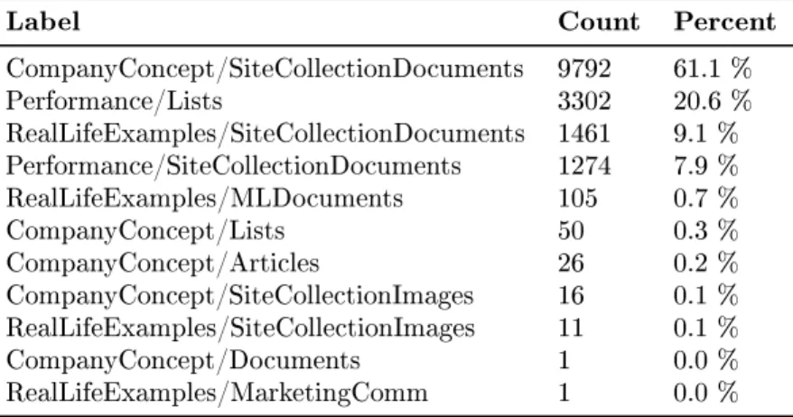
Table 5: Number of documents belonging to each label according to the ground truth. Level = 1. Note how almost 98 % of all documents belong to

the four most popular labels.

Label Count Percent

CompanyConcept/SiteCollectionDocuments 9792 61.1 % Performance/Lists 3302 20.6 % RealLifeExamples/SiteCollectionDocuments 1461 9.1 % Performance/SiteCollectionDocuments 1274 7.9 % RealLifeExamples/MLDocuments 105 0.7 % CompanyConcept/Lists 50 0.3 % CompanyConcept/Articles 26 0.2 % CompanyConcept/SiteCollectionImages 16 0.1 % RealLifeExamples/SiteCollectionImages 11 0.1 % CompanyConcept/Documents 1 0.0 % RealLifeExamples/MarketingComm 1 0.0 %

(32)

4.2 K-Means (Sherlock)

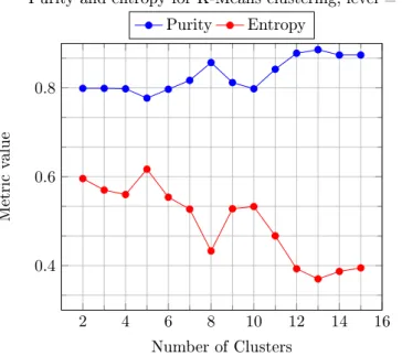
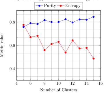
The data used to create all plots in this section can be found in tables 9 and 10. Figures 5 and 6 were created from Sherlock runs that were told to create dierent numbers of clusters, seen on thexaxis. The metrics purity and entropy can be

calculated per clustering in our system, that is why they are presented separately from the others. The metrics were calculated with the level (explained in 3.4.2) set to zero, producing three dierent labels, and to one, producing eleven dierent labels. 14 2 4 6 8 10 12 14 16 0.4 0.6 0.8 Number of Clusters Metric value

Purity and entropy for K-Means clustering, level = 0. Purity Entropy

Figure 5: Purity and entropy for K-Means clustering. We expect a local maximum for purity

and minimum for entropy at nc = 3, since that is how many labels we have at level zero. Note that a

low entropy means a better clustering.

(33)

4 6 8 10 12 14 16 0.4 0.6 0.8 Number of Clusters Metric value

Purity and entropy for K-Means clustering, level = 1. Purity Entropy

Figure 6: Purity and entropy for K-Means clustering. We expect a local maximum for purity and minimum for entropy at nc = 11, since that is how many labels we have at level one. Note that a

(34)

2 4 6 8 10 12 14 16 0.2 0.4 0.6 Number of Clusters Metric value

Homogeneity, completeness and V-measure scores for K-Means clustering, level = 0.

cs hs vms

Figure 7: Homogeneity, completeness and V-measure scores for K-Means clustering with dierent number

of clusters. Metrics calculated with level = 0, meaning there are three labels.

The next two gures (7 and 8) show the three correlated metrics homogene-ity, completeness and V-measure score (hs, cs and vms). Just as before the metrics were calculated with the level set to zero and to one.

The nal two gures for K-Means 9 and 10 show all the broad metrics for cluster performance. Just as before the metrics were calculated with the level set to zero and to one.

(35)

4 6 8 10 12 14 16 0.2 0.4 0.6 Number of Clusters Metric value

Homogeneity, completeness and V-measure scores for K-Means clustering, level = 1.

cs hs vms

Figure 8: Homogeneity, completeness and V-measure scores for K-Means clustering with dierent number

of clusters. Metrics calculated with level = 1, meaning there are eleven labels. We therefore expect

a local maximum at nc = 11.

Table 6: Purity, entropy and size for individual K-Means clusters with number of clusters set to three 3 and level set to 0. Cluster 2 is perfet and

cluster 1 is almost perfect. cluster purity entropy size

0 0.723 0.782 11664

1 0.999 0.008 2929

2 1.000 0.000 1446

For some limits and values for number of clusters (nc) the individual cluster purity, entropy and size are interesting to discuss. This data is displayed in tables 6, 7 and 8.

(36)

2 4 6 8 10 12 14 16 0 0.2 0.4 0.6 0.8 Number of Clusters Metric value

The vms, ars and fms for K-Means clustering, level = 0.

vms ars fms

Figure 9: V-measure score, Adjusted Rand score and Fowlkes Mallows score for K-Means clustering. Local maximums are exected at nc = 3, since that is

how many labels there are at level zero. Note that fms is unreliable for low values of nc. Table 7: Purity, entropy and size for K-Means clusters with number of clusters set to 8 and level

set to 0.

cluster purity entropy size

0 0.719 0.763 3085 1 1.000 0.000 1527 2 1.000 0.000 1362 3 0.809 0.593 1475 4 0.839 0.531 6158 5 0.999 0.009 866 6 0.864 0.408 1070 7 1.000 0.000 496

(37)

4 6 8 10 12 14 16 0 0.2 0.4 0.6 0.8 Number of Clusters Metric value

The vms, ars and fms for K-Means clustering, level = 1.

vms ars fms

Figure 10: V-measure score, Adjusted Rand score and Fowlkes Mallows score for K-Means clustering. Local maximums are expected at nc = 11, since that

is how many labels there are at level one. Note that fms is unreliable for low values of nc. Table 8: Purity, entropy and size for K-Means clusters with number of clusters set to 11 and level

set to 1.

cluster purity entropy size

0 0.996 0.026 496 1 1.000 0.000 411 2 0.863 0.421 1057 3 0.961 0.186 516 4 0.959 0.201 615 5 0.990 0.061 866 6 0.999 0.007 1116 7 1.000 0.000 1317 8 0.527 1.115 1394 9 0.790 0.716 5367 10 0.715 0.872 2884

(38)

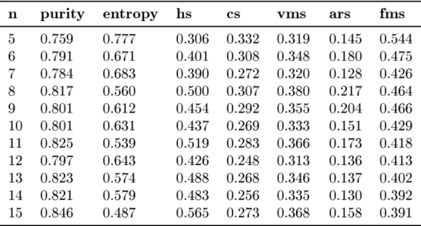
Table 9: All metrics for K-Means clustering with number of clusters set to dierent values. Metrics

were calculated with level set to 0.

nc purity entropy hs cs vms ars fms

2 0.799 0.596 0.326 0.605 0.424 0.404 0.754 3 0.799 0.570 0.356 0.414 0.383 0.277 0.653 4 0.798 0.560 0.366 0.329 0.347 0.223 0.593 5 0.777 0.617 0.302 0.233 0.263 0.156 0.542 6 0.797 0.554 0.373 0.220 0.277 0.140 0.461 7 0.817 0.527 0.404 0.280 0.331 0.214 0.568 8 0.857 0.433 0.510 0.253 0.338 0.223 0.488 9 0.812 0.528 0.403 0.201 0.268 0.131 0.429 10 0.798 0.533 0.398 0.189 0.256 0.086 0.389 11 0.842 0.467 0.472 0.216 0.297 0.137 0.424 12 0.878 0.393 0.556 0.240 0.335 0.211 0.468 13 0.886 0.370 0.582 0.233 0.333 0.166 0.418 14 0.874 0.387 0.562 0.207 0.303 0.123 0.357 15 0.874 0.395 0.553 0.213 0.307 0.158 0.409

Table 10: All metrics for K-Means clustering with number of clusters set to dierent values. Metrics

were calculated with level set to 1.

n purity entropy hs cs vms ars fms

5 0.759 0.777 0.306 0.332 0.319 0.145 0.544 6 0.791 0.671 0.401 0.308 0.348 0.180 0.475 7 0.784 0.683 0.390 0.272 0.320 0.128 0.426 8 0.817 0.560 0.500 0.307 0.380 0.217 0.464 9 0.801 0.612 0.454 0.292 0.355 0.204 0.466 10 0.801 0.631 0.437 0.269 0.333 0.151 0.429 11 0.825 0.539 0.519 0.283 0.366 0.173 0.418 12 0.797 0.643 0.426 0.248 0.313 0.136 0.413 13 0.823 0.574 0.488 0.268 0.346 0.137 0.402 14 0.821 0.579 0.483 0.256 0.335 0.130 0.392 15 0.846 0.487 0.565 0.273 0.368 0.158 0.391

(39)

4.3 SVM (Mycroft)

In this section all metrics for the SVM classication are presented. The data has been calculated using the test data (25 % of the data) from the cross-validate split, and not the training data.

Table 11 shows the number of clusters created for dierent SVM methods. Table 11: Number of distinct labels categorized by

the SVM by level and kernel function. For level 0 the documents had 3 distinct labels during training and validation. As we can see in this table the linear

kernel function managed to separate and predict all the 3 dierent classes. For level 1 the number of

distinct labels was 11.

Level Linear RBF SIGMOID Poly

Level 0 3 2 1 1

(40)

level0 level1 0 0.2 0.4 0.6 0.8 1 1.2 Metric value

Entropy for dierent SVM kernel functions and levels.

Linear RBF Sigmoid Poly Figure 11: The entropy calculated for the dierent

kernel functions at two dierent levels. Level 0 corresponds to 3 distinct labels during training, level

1 corresponds to 11 distinct labels during training. Interesting to note here is that the entropy for the linear kernel function is much lower than the others.

(41)

level0 level1 0 0.2 0.4 0.6 0.8 1 Metric value

Purity for dierent SVM kernel functions and levels.

Linear RBF Sigmoid Poly Figure 12: The purity calculated for the dierent

kernel functions at two dierent levels. Level 0 corresponds to 3 distinct labels during training, level

1 corresponds to 11 distinct labels during training. Interesting to note here is that the entropy for the linear kernel function is much lower than the others.

(42)

purit y en trop y _hs _cs vms ars fms 0 0.2 0.4 0.6 0.8 1 1.2 Metric value

All metrics for dierent SVM kernel functions, level = 0.

Linear RBF Sigmoid Poly Figure 13: The other metrics for level 0. This is table 12 in plot format. Note that for metrics but

entropy a high value is a good score.

Figures 11 and 12 show the purities and entropies of the SVM classication. Summaries of all metrics, for level 0 and level 1, can be found in gures 13 and 14. The underlying data can bee seen in tables 12 and 13.

Table 12: All metrics for SVM clustering with dierent kernels. Level is set to 0.

Measure Linear RBF SIGMOID Poly purity 0.942 0.803 0.608 0.615 entropy 0.235 0.587 0.896 0.882 hs 0.734 0.331 0.000 0.000 cs 0.801 0.612 1.000 1.000 vms 0.766 0.429 0.000 0.000 ars 0.834 0.411 0.000 0.000 fms 0.917 0.759 0.681 0.686

(43)

purit y en trop y _hs _cs vms ars fms 0 0.2 0.4 0.6 0.8 1 1.2 Metric value

All metrics for dierent SVM kernel functions, level = 1.

Linear RBF Sigmoid Poly Figure 14: The other metrics for level 1. This is table 13 in plot format. Note that for metrics but

entropy a high value is a good score. Table 13: All metrics for SVM clustering with

dierent kernels. Level is set to 1.

Measure Linear RBF SIGMOID Poly purity 0.942 0.784 0.606 0.611 entropy 0.254 0.755 1.115 1.122 hs 0.775 0.333 0.000 0.000 cs 0.859 0.809 1.000 1.000 vms 0.815 0.471 0.000 0.000 ars 0.854 0.427 0.000 0.000 fms 0.920 0.756 0.653 0.655

4.4 Comparing K-Means and SVM

In order to compare the two methods some plots were created. They display best selection of K-Means computations compared with SVM computations, in terms of all of the previously discussed metrics. Figures 15 and 16 show the more general metrics in order to asses which clustering is better, and 17 and 18 the more aspect specic metrics in order to analyze how they dier.

(44)

vms ars _fms 0 0.2 0.4 0.6 0.8 1 Metric value

vms, ars and fms for K-Means and SVM, level = 0.

SVM K-Means

Figure 15: V-measure, Adjusted Rand index and Fowlkes Mallows score for K-Means and SVM,

calculated with level = 0 (3 labels).

vms ars _fms 0 0.2 0.4 0.6 0.8 1 Metric value

vms, ars and fms for K-Means and SVM, level = 1.

SVM K-Means

Figure 16: V-measure, Adjusted Rand index and Fowlkes Mallows score for K-Means and SVM,

(45)

purity entropy hs cs 0 0.2 0.4 0.6 0.8 1 Metric value

Purity, entropy, hs and cs for K-Means and SVM, level = 0.

SVM K-Means

Figure 17: Purity, Entropy, Homogeneity and Completeness scores for K-Means and SVM,

calculated with level = 0 (3 labels).

purity entropy hs cs 0 0.2 0.4 0.6 0.8 1 Metric value

Purity, entropy, hs and cs for K-Means and SVM, level = 1.

SVM K-Means

Figure 18: Purity, Entropy, Homogeneity and Completeness scores for K-Means and SVM,

(46)

4.5 Similar documents (Deduction)

There are no quantiable results on the similar documents part of the project since other parts were prioritised. However, the screenshot in gure 19 shows how the results are displayed on the platform.

Figure 19: Screenshot from the platform, showing the related documents feature in application.

4.6 Visualizing Clusters

4.6.1 Magnier

Since Magnier is just a tool for navigating and examining the corpus and clus-tering, there is no mathematical presentation of it to present. A few screenshots were created to visualize the tool, in order to be able to discuss its usefulness. 4.6.2 Grid cluster preview

The grid cluster preview is an alternate way to view and assess the clustering. It randomly selects a number of documents from each cluster and then displays their rst page as a thumbnail image. Note that some documents do not have previews available. The visualizations can be found in the appendix, gures 23 to 39. The previews have been pixelated in this report.