Munich Personal RePEc Archive
Oil price assumptions for macroeconomic
policy
Degiannakis, Stavros and Filis, George
Panteion University of Social and Political Sciences, Department of
Economic and Regional Development, Bournemouth University,
Department of Accounting, Finance and Economics
27 May 2020
Online at
https://mpra.ub.uni-muenchen.de/100705/
MPRA Paper No. 100705, posted 28 May 2020 17:25 UTC
Oil price assumptions for macroeconomic policy
Stavros Degiannakis1 and George Filis2,*
1Panteion University of Social and Political Sciences, Department of Economic and Regional
Development, Syggrou Avenue 136, 176721, Athens, Greece
2Bournemouth University, Department of Accounting, Finance and Economics, 89
Holdenhurst Road, Executive Business Centre, BH8 8EB, Bournemouth, UK *Corresponding author’s email: gfilis@bournemouth.ac.uk
Abstract
Despite the arguments that are put forward by the literature that oil price forecasts are economically useful, such claim has not been tested to date. In this study we evaluate the economic usefulness of oil price forecasts by means of conditional forecasting of three core macroeconomic indicators that policy makers are predicting, using assumptions about the future path of the oil prices. The chosen indicators are the core inflation rate, industrial production and purchasing price index. We further consider two more indicators, namely inflation expectation and monetary policy uncertainty. To do so, we initially forecast oil prices using a MIDAS framework and subsequently we use regression-based models for our conditional forecasts. Overall, there is diminishing importance of oil price forecasts for macroeconomic projections and policy formulation. An array of arguments is presented as to why this might be the case, which relate to the improved energy efficiency, the contemporary monetary policy tools and the financialisation of the oil market. Our findings remain robust to alternative oil price forecasting frameworks.
Keywords: Conditional forecasting, oil price forecasts, MIDAS, core inflation, inflation expectations.
1. Introduction
The aim of this paper is to extend the rather rich literature on oil price forecasting and the state-of-the-art forecasting approaches, concentrating for the first time on the economic usefulness of such forecasts, via conditional forecasting of macroeconomic indicators.
The extant literature supports that oil price forecasting is important for a number of stakeholders, including policy makers (such as central banks), firms and households (Elder and Serletis, 2010; Bauimeister et al., 2014), given the role that oil prices play on several aspects of economic activity. More specifically, the literature suggests that oil price fluctuations (i) could exert a significant impact on growth paths, balance of payments and inflation, among others1 and (ii) could also offer predictive power for the aforementioned economic variables, as well as, sentiment indicators2.
For instance, Baumeister and Kilian (2014, p.869) maintain that “changes in the cost of imported crude oil are an important determinant of economic activity, which is why central banks worldwide and international organizations such as the International Monetary Fund (IMF) routinely rely on real-time forecasts of the price of oil in assessing the economic outlook”and that “central banks rely on forecasts of the real price of oil when making policy decisions. (p.886)”. Even more, Baumeister et al. (2014, p.S33) further suggests that “accurate real-time forecasts of the price of oil are important to firms and consumers as well as state and national governments.”, whereas, Baumeister et al. (2018, p.562) inform us that “users of oil price forecasts include international organizations, central banks, governments at the state and federal level as well as a range of industries including utilities and automobile manufacturers.”
International institutions, central banks, as well as, global media also link the macroeconomic stability with oil price fluctuations. The IMF (2016), for example, supports that the deflationary pressures in the early part of the 2010s that was particularly observed in oil-importing countries, were caused by the significant drop in oil prices. Such deflationary pressures impose further constraints to central banks to support growth to fragile economies, due to the low interest rate environment. It is also indicatively that IMF (2016) further claims that prolong periods of low oil prices could also halt the economic growth of oil-exporting economies. Similarly, the ECB (2016a) provides evidence of the impact of the oil price slump on the fiscal policy stance of oil producers, since for many of them, oil prices are well below their fiscal breakeven prices.
1 See, inter alia, Backus and Crucini (2000), Aguiar‐Conraria and Wen (2007), Hamilton (2008), Kilian et al. (2009), Bachmeier and Cha (2011), Natal (2012) and Jo (2014).
The global media, on the other hand, raise concerns as to how successful the ECB could be in raising inflation rates for 2016-2018 given the low oil prices (Barnato, 2016), whereas, Blas and Kennedy (2016) raise even more concerns maintaining that should energy prices continue to fall, then the world economy might enter into a tailspin.
Given the aforementioned indicative quotes and policy statements, which highlight the importance of oil price fluctuations and thus, oil price forecasts, it is rather interesting that the related literature has neglected to assess the economic usefulness of such forecasts. This is even more interesting when in fact Alquist et al. (2013) suggest that successful oil price forecasts have the potential to improve the forecasts for an array of macroeconomic variables, which could further lead to better policy responses; nevertheless, we observe that such claim has not been put into the test. More recently, Kilian and Vigfusson (2017) also opine that in order to provide an answer as to which model specification of oil price is more appropriate for policy making, this should be made based on model selection criteria rather than statistical testing. Thus, modelling frameworks for oil prices should be ranked according to their conditional performance relatively to a macroeconomic variable. At the same time, they highlight that the conditional performance of modelling frameworks in this line of research has been remained largely unexplored.
Despite the important points raised by Alquist et al. (2013) and Kilian and Vigfusson (2017), it is rather evident that existing studies concentrate on statistical loss functions in order to evaluate their oil price forecasts, ignoring their economic usefulness. Typically, the current practice is to use loss functions, such as the mean squared predictive error (MSPE) or the mean absolute predictive error (MAPE), irrespectively of the different forecasting frameworks that are used to forecast oil prices, i.e. futures-based forecasts (see, for instance, Alquist and Kilian 2010; Alquist et al., 2013), forecasts based on oil price fundamentals (see, for example, Baumeister and Kilian 2012; 2014; 2015; Baumeister et al., 2015; Degiannakis and Filis, 2018) or even based on financial data (see, Baumeister et al., 2015; Degiannakis and Filis, 2018). A recent review of the related literature can be found in Degiannakis et al. (2018a).
Thus, our paper fills this void by assessing oil price forecasts based on their ability to provide successful predictions for a wide range of macroeconomic indicators, which are at the core interest of policy makers, using conditional forecasting. Hence, for the first time in the bulk literature, we assess the economic usefulness of oil price forecasts.
It should be noted here that it is common practice for central banks to consider oil prices as an exogenous variable and thus, certain assumptions are made related to their future level, when it comes to macroeconomic projections (Coimbra and Esteves, 2004). ECB (2016b)
clearly states that for all their projection exercises they proceed to certain macroeconomic assumptions, such as the future path of oil prices. A key issue, though, with the use of oil futures prices is that they tend to exhibit fairly large projection errors on macroeconomic variables (ECB, 2015).
Thus, in this paper we first forecast oil prices using the current state-of-the-art frameworks and subsequently we use these forecasts as assumptions of the future path of oil prices, so as to generate conditional forecasts for several macroeconomic indicators, including, inflation, industrial production and producers price index. We should highlight that the usefulness of conditional forecasting for macroeconomic variables has been well established, given that “prior knowledge, […], of the future evolution of some economic variables may contain information for the outlooks of other variables” (see, for instance, Bańbura et al., 2015, p. 740). Giannone et al. (2014, p.636) also maintains that conditional forecasts “allows for an […] outlook that is set within (and thus affected by) a clearly-described, albeit imperfectly known in advance, macroeconomic environment”. Such macroeconomic environment could include the future path of oil prices.
As aforementioned, for the first step of our analysis we follow the current state-of-the-art modelling approaches for oil price forecasting, which maintain that the use of oil price volatility, based on high-frequency data, along with oil price fundamentals in lower frequency, can improve oil price forecasts (e.g. Degiannakis and Filis, 2018). Thus, motivated by these recent efforts, we employ a MIDAS framework to forecast the monthly WTI crude oil prices using the predictive information of various WTI realised volatility measures, as well as, the WTI implied volatility index (i.e. OVX index)3. The use of oil price volatility as potential
predictor of oil prices is also motivated by ECB (2015), which suggests that the increased oil price volatility, over the last decade or so, has severe implications for oil price forecasting. For robustness purposes we also use the standard VAR and Bayesian VAR models, as these have been developed by Kilian and co-authors.
The remaining of the paper is structured as follows. Section 2 describes the data. Section 3 details the econometric approach employed in this paper and the conditional forecasting techniques. Section 4 provides a detailed analysis of the findings. Section 5 presents the results from additional monetary policy indicators and Section 6 includes the robustness check using alternative forecasting frameworks. Finally, Section 7 concludes the study.
3 We should note here that previous research solely uses the typical realized volatility measure by Andersen and Bollerslev (1998), whereas the present study uses a wide range of realised and implied oil price volatilities, given that different volatility measures could provide different predictive information for oil prices.
2. Oil price forecasting framework 2.1 Data description
To perform our analysis, we use data at both ultra-high and low frequency. Starting from the former, we use tick-by-tick data for the front-month WTI futures contracts, which are transformed into intraday time-series (ultra-high frequency) so as to allow us the construction of the daily WTI volatility measures (high frequency). The specific volatility measures are presented in Section 2.2. Apart from the daily WTI realised volatility measures, we further use the daily prices of the OVX index, which is the WTI’s implied volatility index. These volatility measures serve as our high-frequency predictors.
The low-frequency (i.e. monthly) predictors include the oil market fundamentals, namely, the global economic activity index (as proxy of the global business cycle), the global oil stocks (as proxies of oil inventories) and the global oil production. Motivated by Degiannakis and Filis (2018), we also use the capacity utilisation rate of the oil and gas industry, since it has been shown by Kaminska (2009) that there is a strong link between the capacity utilisation rate and oil prices.
As for the construction of our predicted variable, i.e. the monthly crude oil prices, we depart from the common practice of the literature, which is based on the average daily prices on any given month (see, for instance, Baumeister and Kilian, 2014, 2015; Naser, 2016; Zhang
et al., 2018), as these averages result in high first-order autocorrelation, which, artificially enhances the predictive ability of the modelling framework. Thus, by contrast, we construct our monthly crude oil prices from the tick-by-tick data. In particular, the monthly WTI oil price is considered to be the futures price of the last intraday observation of each month.
The period of the study spans from 4th January 2010 until 30th October 2017 and it is dictated by the availability of the ultra-high-frequency data (i.e. 1971 daily and 94 monthly observations). The tick-by-tick data are obtained from TickData, whereas the data for the OVX implied volatility index are retrieved from the CBOE.
2.2. WTI intraday realised volatility measures
Based on the literature, we have estimated seven variations of realized volatility, those with the greatest influence in financial modelling. Each proposed measure has each own advantages and disadvantages and, most importantly, the information they provide as explanatory variables diversifies. Let us denote as 𝑟𝑡,𝑖 = 𝑙𝑜𝑔(𝑃𝑡,𝑖) − 𝑙𝑜𝑔(𝑃𝑡,𝑖−1), the 𝑖𝑡ℎ intraday return (for i=1,…,τ) at day t, with τ number of intervals within a trading day. The 𝑃𝑡,𝑖
is the 𝑖𝑡ℎ intraday asset price at day t. The seven intraday realized volatility measures
𝐼𝑅𝑉𝑡: {𝑅𝑉𝑡, 𝑅𝑉𝑡(𝑠), 𝑅𝑉𝑡(𝑏), 𝑅𝑉𝑡(𝑚𝑒𝑑), 𝑅𝑉𝑡(𝑚𝑖𝑛), 𝑅𝑉𝑡(+), 𝑅𝑉𝑡(−)} follow:
1. Andersen and Bollerslev’s (1998) Realized Volatility (𝑅𝑉𝑡):
𝑅𝑉𝑡 = ∑𝜏𝑖=1𝑟𝑡,𝑖2 , (1)
2. Hansen and Lunde’s (2005) Scaled Realized Volatility (𝑅𝑉𝑡(𝑠)):
𝑅𝑉𝑡(𝑠) = 𝜔1(𝑙𝑜𝑔𝑃𝑡,1− 𝑙𝑜𝑔𝑃𝑡−1,𝜏) + 𝜔2∑𝜏𝑖=1𝑟𝑡,𝑖2, (2)
where the parameters 𝜔1 and 𝜔2 are estimated such as min
(𝜔1,𝜔2)𝑉(𝑅𝑉𝑡 (𝑠)), because arg min (𝜔1,𝜔2) 𝐸(𝑅𝑉𝑡 (𝑠)− 𝐼𝑉𝑡) = arg min (𝜔1,𝜔2)
𝑉(𝑅𝑉𝑡(𝑠)), and 𝐼𝑉𝑡 denotes the integrated volatility. 3. Barndorff-Nielsen and Shephard’s (2004) Realized Bipower Variation (𝑅𝑉𝑡(𝑏)):
𝑅𝑉𝑡(𝑏)= (2/𝜋)−1( 𝜏
𝜏−1) ∑ |𝑟𝜏−1𝑖=1 𝑡,𝑖||𝑟𝑡,𝑖+1| , (3)
4. Andersen’s et al. (2012) Median Realized Volatility (𝑅𝑉𝑡(𝑚𝑒𝑑)):
𝑅𝑉𝑡(𝑚𝑒𝑑) = 𝜋 6 − 4√3 + 𝜋( 𝜏 𝜏 − 2) ∑ 𝑚𝑒𝑑(|𝑟𝑡,𝑖−1|, |𝑟𝑡,𝑖| 𝜏−1 𝑖=2 , |𝑟𝑡,𝑖+1|)2, (4)
5. Andersen’s et al. (2012) Minimum Realized Volatility (𝑅𝑉𝑡(𝑚𝑖𝑛)):
𝑅𝑉𝑡(𝑚𝑖𝑛) =𝜋−2𝜋 (𝜏−1𝜏 ) ∑𝜏−1𝑖=1𝑚𝑖𝑛(|𝑟𝑡,𝑖|,|𝑟𝑡,𝑖+1|)2. (5)
6. Barndorff-Nielsen et al. (2010) Positive Semi Variance (𝑅𝑉𝑡(+)):
𝑅𝑉𝑡(+) = ∑𝜏𝑖=1𝛪{𝑟𝑡,𝑖 ≥ 0}𝑟𝑡,𝑖2 , (6)
where 𝛪{. } is an indicator function taking the value 1 if the argument is true. 7. Barndorff-Nielsen et al. (2010) Negative Semi Variance (𝑅𝑉𝑡(−)):
𝑅𝑉𝑡(−)= ∑𝜏𝑖=1𝛪{𝑟𝑡,𝑖 < 0}𝑟𝑡,𝑖2 . (7)
The realized variance, 𝑅𝑉𝑡, is the most known estimator of intraday realized volatility on a daily sampling frequency and it has been applied in all the financial studies that focus on volatility predictions.
The 𝑅𝑉𝑡(𝑠) has successfully introduced the combination of intraday volatility during the open-to-closed period with the closed-to-open inter-day volatility. Among the various modifications that have been suggested for the overnight adjustment of realized volatility, i.e. Blair et al. (2001), Martens (2002), Koopman et al. (2004), the 𝑅𝑉𝑡(𝑠) estimates the weight of
overnight volatility based on the minimization of the expected distance between computed 𝑅𝑉𝑡 and latent (thus, unobservable) 𝐼𝑉𝑡.
Barndorff-Nielsen and Shephard (2004 and 2006) showed that the 𝑅𝑉𝑡(𝑏) is an estimator of the integrated volatility 𝐼𝑉𝑡 in the presence of jumps. So, if we assume that the intraday asset price follows a jump-diffusion process, then the volatility includes a jump component and the quadratic variation 𝑄𝑉𝑡 equals to the integrated volatility plus the jump variation; or 𝑄𝑉𝑡=
∫ 𝜎𝑠2𝑑𝑠 + ∑ 𝜅𝑠2 𝑡−1<𝑠≤𝑡 𝑡
𝑡−1 . The bipower variation is robust to the presence of jumps and we can
combine realized variance with bipower variation to estimate the jump variation components. The 𝑅𝑉𝑡(𝑚𝑒𝑑) and 𝑅𝑉𝑡(𝑚𝑖𝑛), proposed by Andersen et al. (2012), also provide estimates for integrated variance in the presence of jumps. Both are more robust estimators than the 𝑅𝑉𝑡(𝑏) and its multipower variations due to the fact that large absolute returns associated with jumps tend to be eliminated from the calculation of the median and minimum operators; see also Theodosiou and Zikes (2009). When infrequent jumps are present the 𝑅𝑉𝑡(𝑚𝑒𝑑) is less sensitive to the existence of zero intraday returns and it has better efficiency properties than the tripower variation.
The 𝑅𝑉𝑡(+) and 𝑅𝑉𝑡(−)capture the variation solely from positive and negative returns. Patton and Sheppard (2015) provided evidence that for equity data, the downside realized semi-variance is much more important for forecasting future volatility than the positive realized semi-variance.
Apart from these realized volatility measures, we further consider the difference between the positive and negative semi variance (𝑅𝑉𝑡(𝑆𝐽)= 𝑅𝑉𝑡(+)− 𝑅𝑉𝑡(−)), the OVX index, as well as, the variance risk premiums (𝑉𝑅𝑃𝑡) according to Bollerslev et al. (2009), as follows:
𝑉𝑅𝑃𝑡 = 𝑂𝑉𝑋𝑡− 𝐼𝑅𝑉𝑡, (8)
where, 𝑂𝑉𝑋𝑡 is the WTI implied volatility and 𝐼𝑅𝑉𝑡 denotes each of the seven (7) different intraday realized volatility measures mentioned in this section, i.e.
𝐼𝑅𝑉𝑡: {𝑅𝑉𝑡, 𝑅𝑉𝑡(𝑠), 𝑅𝑉𝑡(𝑏), 𝑅𝑉𝑡(𝑚𝑒𝑑), 𝑅𝑉𝑡(𝑚𝑖𝑛), 𝑅𝑉𝑡(+), 𝑅𝑉𝑡(−)}.
The motivation for using of the variance risk premiums (𝑉𝑅𝑃𝑡), as additional predictors for oil price forecasts, stems from the fact that this relatively newly developed volatility measure has gained prominence in the finance literature in relation to its ability explaining asset price fluctuations (see, Carr and Wu, 2008; Bollerslev et al., 2009; Prokopczuk, 2017). Even more, the 𝑉𝑅𝑃𝑡is able to gauge investors’ fear of a potential market crash (Tee and Ting,
2017). Thus, we maintain that the oil futures 𝑉𝑅𝑃𝑡 could provide incremental predictive information for the future path of oil prices. In total we consider 16 volatility measures.
As the trading frequency increases substantially, i.e. →, the market frictions impose additional noise in volatility estimates. Given the availability of the tick-by-tick data, we construct time series per 5-second intervals and we compute the intraday autocovariance, 𝐶𝑜𝑣(𝑟𝑡,𝑖, 𝑟𝑡,𝑖−𝑗) = ∑𝜏−1𝑗=1∑𝜏𝑖=𝑗+1𝑟𝑡,𝑖𝑟𝑡,𝑖−𝑗, across sampling frequencies. Looking for the sampling frequency that minimizes the autocovariance bias, we find that the trade-off between accuracy and potential bias induced by microstructure frictions is achieved at 20-minutes for the WTI realized volatility.
An obvious question would be why we consider the different realised volatility measures to forecast oil prices. It would make sense only if they provide different information to oil prices. Figures 1 and 2 show the WTI oil prices along with selected measures of WTI price volatility. Figure 1 reveals that there are no material differences among either the volatility measures or the variance risk premiums. For instance, all the three chosen volatility measure seem to peak during 2011, given the economic turbulence in the Eurozone, as well as, during the oil price collapse of 2014-2016. A notable difference is only on the fact that the OVX seems to be less volatile compared to the intraday realised volatility measures, which is rather anticipated. Even more, the two chosen variance risk premiums also exhibit similar behaviour, with major troughs in the two aforementioned periods.
Nevertheless, to motivate our choice of using the different volatility measures we show Figure 2, which depicts the same volatility measures as in Figure 1, yet only for a randomly selected month. The visual inspection of Figure 2 clearly shows that the different volatility measures could incorporate different information, given that their behaviour is not necessarily similar.
[FIGURES 1 and 2 HERE]
2.3. The MIDAS framework for oil price forecasting
Motivated by Baumeister et al. (2015) and Degiannakis and Filis (2018), we model the future monthly crude oil prices to be driven by high-frequency data (oil price volatility in our case) along with low-frequency oil price fundamentals. The high-frequency oil volatility information set includes the various WTI realised volatility measures that we have computed; i.e. {𝑅𝑉𝑡, 𝑅𝑉𝑡(𝑠), 𝑅𝑉𝑡(𝑏), 𝑅𝑉𝑡(𝑚𝑒𝑑), 𝑅𝑉𝑡(𝑚𝑖𝑛), 𝑅𝑉𝑡(+), 𝑅𝑉𝑡(−)}, the 𝑅𝑉𝑡(𝑆𝐽), the WTI implied volatility index; i.e. 𝑂𝑉𝑋𝑡, as well as, the variance risk premiums. The 𝐺𝐸𝐴𝑡, 𝑃𝑟𝑜𝑑𝑡, 𝑆𝑡𝑜𝑐𝑘𝑠𝑡
and 𝐶𝑎𝑝𝑡 denote the global economic activity, the global oil production, the global oil stocks and the capacity utilisation rate, respectively, at a monthly frequency.
Let us denote as 𝛥(𝑂𝑖𝑙𝑡) = 𝑙𝑜𝑔(𝑂𝑖𝑙𝑡⁄𝑂𝑖𝑙𝑡−1) the oil futures price monthly returns, as
𝑭𝑡= (𝐺𝑒𝑎𝑡, 𝑙𝑜𝑔(𝑃𝑟𝑜𝑑𝑡⁄𝑃𝑟𝑜𝑑𝑡−1), 𝑙𝑜𝑔(𝑆𝑡𝑜𝑐𝑘𝑠𝑡⁄𝑆𝑡𝑜𝑐𝑘𝑠𝑡−1), 𝐶𝑎𝑝𝑡)′, the vector of
fundamental explanatory variables at a monthly frequency and as 𝑽𝑶𝑳(𝑡)(𝐷) the vector of realized volatilities, the 𝑅𝑉𝑡(𝑆𝐽), the OVX and variance risk premiums. The MIDAS model was built in order to regress the monthly dependent variable directly with the monthly explanatory variables, 𝑭𝑡, and via the polynomial distributed lag weighting with the daily realized volatilities, 𝑽𝑶𝑳(𝑡)(𝐷):
𝛥(𝑂𝑖𝑙𝑡) = 𝑭′𝑡−𝑖𝜷 + ∑ 𝑽𝑶𝑳(𝑡−𝑟−𝑖𝑠)′(𝐷) (∑𝑝 𝑟𝑗𝜽𝑗 𝑗=0 ) 𝑘−1
𝑟=0 + 𝜀𝑡. (9)
The error term is assumed to be normally distributed, 𝜀𝑡~𝑁(0, 𝜎𝜀2), the 𝜷, 𝜽𝑗 are vectors of coefficients to be estimated, and the 𝑠 = 22 denotes the number of daily observations at each month.
The current’s month oil futures price is related with a) the oil price fundamentals up to
𝑖 months before and b) the volatility measures up to 𝑖𝑠 + 𝑟 trading days before. The variables have been constructed and their relationship with the dependent variable was established such as to avoid any possible looking ahead bias. Thus, we are able to estimate up to 𝑖 months-ahead oil futures price forecasts without imposing the utilization of future actual information from explanatory variables. I.e., we set 𝑖 ≥ 1 (as well as 𝑖𝑠 ≥ 22) in order to predict the one-month ahead oil price. Additionally, we set 𝑖 ≥ 6 and 𝑖𝑠 ≥ 132, when we predict the six-months ahead oil price and so on.
Moreover, 𝑘, which is the number of lagged days to be employed, is estimated such as to minimize the in-sample sum of squared residuals. Additionally, the dimension of the lag polynomial in the vector parameters 𝜽𝑗, denoted as 𝑝, has been investigated with a series of in-sample evaluation tests and was set equal to three. Henceforth, we avoid inducing a form of data mining bias, which would have been the case if we had estimated the k and 𝑝 that minimize the sum of squared forecast errors in the out-of-sample period.
3. Evaluating oil price forecasts based on conditional forecasting
As aforementioned in Section 1, the aim of this study is to evaluate the economic usefulness of oil price forecasts by means of conditional forecasting. To do so, we focus on three core macroeconomic indicators that policy makers are forecasting, using assumptions
about the future path of the oil prices. These indicators are the inflation rate, industrial production and purchasing price index. We shall reiterate that our oil price forecasts are used as assumptions in the following conditional forecasting framework.
3.1. Data description for conditional forecasting
To proceed with the conditional forecasts of core inflation, we use monthly data for the period January 2010 to October 2017 for the US core CPI and the US unemployment gap. The unemployment gap is measured as the difference between the US unemployment rate and the nonaccelerating inflation rate of unemployment (NAIRU). Furthermore, monthly data for the same period are obtain for the industrial production and purchasing price indices. All data are obtained from the Federal Reserve of St. Luis (Federal Reserve Economic Data).
3.2. Conditional forecasting framework for macroeconomic conditions 3.2.1. Inflation
Typically, the literature estimates an augmented Philips curve to assess the impact of oil prices on inflation, such as:
𝜋𝑡= 𝑎 + ∑𝐼𝑖=1𝛽𝑖𝜋𝑡−𝑖+ 𝛾(𝑢𝑛𝑡−1− 𝑛𝑎𝑖𝑟𝑢𝑡−1) + ∑ 𝛿𝑖𝐼𝑖=0 𝛥(𝑂𝑖𝑙𝑡−𝑖)+ 𝑒𝑡, (10)
where, 𝜋𝑡 denotes the core inflation rate at month t, 𝑢𝑛𝑡 is the US unemployment rate, 𝑛𝑎𝑖𝑟𝑢𝑡 is the nonaccelerating inflation rate of unemployment, hence, (𝑢𝑛𝑡− 𝑛𝑎𝑖𝑟𝑢𝑡) refers to the unemployment gap and 𝛥(𝑂𝑖𝑙𝑡) refers to the crude oil price monthly changes. Finally,
𝑒𝑡~𝑁(0, 𝜎𝑒2) is the error term.
Hooker (2002), for instance, uses the Philips curve to identify the oil price pass-through, whereas, Coibion and Gorodnichencko (2015), using the augmented Philips curve, reveal that inflation rate during the Global Financial Crisis (GFC) increased as a consequence of the increased oil prices at that period. More recently, Gelos and Ustyugova (2017) and Renou-Maissant (2019) also use the augmented Philips curve to identify the effects of oil price changes to inflation rates.
However, the aforementioned studies do not proceed to conditional forecasts of inflation, which reflect the actual needs of policy makers. Thus, we use a variant of eq.(10) so to accommodate the fact that oil price forecasts serve as macroeconomic assumptions for inflation projections, such as that:
𝜋𝑚,𝑡+ℎ = 𝑎 + ∑ 𝛽𝑖𝜋𝑡+ℎ−𝑖 𝐼 𝑖=1 + 𝛾(𝑢𝑛𝑡+ℎ−1− 𝑛𝑎𝑖𝑟𝑢𝑡+ℎ−1) + ∑ 𝛿𝑖𝛥(𝑂𝑖𝑙𝑚,𝑡+ℎ−𝑖|𝑡) 𝐼 𝑖=0 + 𝑒𝑡+ℎ, (11)
where, 𝜋𝑚,𝑡+ℎ denotes the ℎ-step ahead real conditional forecast of the core inflation based on the different oil price forecasting models, 𝑚, (for ℎ = 1, … 12 months). 𝑂𝑖𝑙𝑚,𝑡+ℎ−𝑖|𝑡 denotes the prediction of oil price at month 𝑡 + ℎ, based on each of the 16 models, 𝑚 (i.e. based on the 7 realized volatilities, the 𝑅𝑉𝑡(𝑆𝐽), the OVX and the 7 variance risk premiums), which has been estimated with the available information at month 𝑡. Note that 𝑖 ≥ ℎ should hold in order to avoid any looking-forward bias. Our oil price forecasts from month 𝑡 + 1 up to month 𝑡 + ℎ are estimated iterated based on the information set that is available on month 𝑡:
𝑂𝑖𝑙𝑚,𝑡+ℎ|𝑡= 𝑂𝑖𝑙𝑚,𝑡+ℎ−1|𝑡𝑒(𝑭 ′𝑡−𝑖+ℎ𝜷(𝒕)+∑ 𝑽𝑶𝑳 (𝑡−𝑟−𝑖𝑠) ′(𝐷) (∑ 𝑟𝑗𝜽 𝑗 (𝑡) 𝑝 𝑗=0 ) 𝑘−1 𝑟=0 ), (12)
for ℎ ≥ 2, whereas for ℎ = 1 we predict oil as 𝑂𝑖𝑙𝑚,𝑡+ℎ|𝑡 =
𝑂𝑖𝑙𝑡𝑒(𝑭′𝑡−𝑖+1𝜷(𝒕)+∑𝑟=0𝑘−1𝑽𝑶𝑳(𝑡−𝑟−𝑖𝑠)′(𝐷) (∑𝑝𝑗=0𝑟𝑗𝜽(𝑡)𝑗 )+𝜎̂𝜀 2
2 ⁄ )
. Eq.(11) allows us to evaluate which oil price forecast is performing best based on its ability to provide predictive gains for the core inflation. We note that we estimate eq.(11) for 𝜋𝑡 denoting (i) the log of the consumer price index (𝐶𝑃𝐼𝑡), (ii) the m-o-m changes of 𝐶𝑃𝐼𝑡 and (iii) the y-o-y change of 𝐶𝑃𝐼𝑡4. We do so since we are agnostic as to which transformation of the 𝐶𝑃𝐼 series would provide accurate conditional forecasts of the 𝐶𝑃𝐼 itself.
3.2.2. Industrial Production and Production Price indices
Similarly, to the inflation projection approach, we estimate the following equation to generate conditional forecasts for the industrial production and production price indices, respectively, based on oil price forecasts:
𝑧𝑚,𝑡+ℎ = 𝑎 + ∑ 𝛽𝑖𝑧𝑡+ℎ−𝑖 𝐼 𝑖=1 + ∑ 𝛿𝑖𝛥(𝑂𝑖𝑙𝑚,𝑡+ℎ−𝑖|𝑡) 𝐼 𝑖=0 + 𝑒𝑡+ℎ (13) where, 𝑧𝑚,𝑡+ℎ denotes either the log of industrial production (𝐼𝑃𝑡) or the purchasing price index (𝑃𝑃𝐼𝑡) real conditional forecasts at month 𝑡 + ℎ, based on the different oil price forecasting models. 𝑂𝑖𝑙𝑚,𝑡+ℎ|𝑡 denotes the oil price prediction at month 𝑡 + ℎ given the information available at month 𝑡, and 𝑒𝑡~𝑁(0, 𝜎𝑒2) is the error term. For robustness purposes, we estimate
eq.(13) for 𝑧𝑡 denoting, apart from the log levels, the m-o-m and y-o-y changes of 𝐼𝑃𝑡 and 𝑃𝑃𝐼𝑡, as well.
We note that for economically useful comparisons we also generate conditional forecasts based on the non-oil models, which are the models from eqs. (11) and (13), excluding the information from the oil price forecasts (i.e. ∑𝐼𝑖=0𝛿𝑖𝛥(𝑂𝑖𝑙𝑚,𝑡+ℎ−𝑖|𝑡)).
Thus, in total, for each macroeconomic indicator we estimate 16 MIDAS models, using each one of the WTI realised volatility measures, the 𝑅𝑉𝑡(𝑆𝐽), the OVX and the VRPs, at a time, as well as, the non-oil model.
3.2.3. Validate the Forecasting Accuracy
Being in line with forecasting literature (i.e. Degiannakis et al., 2018b and Marcellino
et al., 2003) and keeping in mind the high non-linearity of the MIDAS model, we use the 2/3
of the available data for the initial in-sample estimation period, 𝑇̆ (January 2010 - November 2014) and the remaining 1/3 of the observations for the out-of-sample evaluation period, 𝑇̃ (December 2014 – October 2017). More technical details regarding the efficient estimation of MIDAS are available in Andreou et al. (2010, 2013) and Ghysels et al. (2006).
To establish the performance of the competing models to forecast 𝐼𝑛𝑑𝑡: {𝜋𝑡, 𝐼𝑃𝑡, 𝑃𝑃𝐼𝑡}, we employ the Model Confidence Set (MCS) of Hansen et al. (2011), which identifies the set of the best models which have equal predictive accuracy, according to a predictive evaluation criterion5. We utilize the two most well-established statistical evaluation criteria, the Mean Squared Predictive Error (MSPE) and the Mean Absolute Predictive Error (MAPE). Let us denote the 𝛹𝑚,𝑡(𝑚𝑠𝑝𝑒) and 𝛹𝑚,𝑡(𝑚𝑎𝑝𝑒) evaluation criteria:
𝛹𝑚,𝑡(𝑚𝑠𝑝𝑒) = (𝐼𝑛𝑑𝑚,𝑡+ℎ|𝑡− 𝐼𝑛𝑑𝑡+ℎ)2, (14)
and
𝛹𝑚,𝑡(𝑚𝑎𝑝𝑒) = |𝐼𝑛𝑑𝑚,𝑡+ℎ|𝑡− 𝐼𝑛𝑑𝑡+ℎ|, (15)
where 𝐼𝑛𝑑𝑚,𝑡+ℎ|𝑡 denotes the prediction of each of the three macroeconomic indicators, based on each of the different oil price forecasts, from model 𝑚, at month 𝑡 + ℎ which has been estimated with the information that is available at month 𝑡. The difference among the forecast error of any two models, 𝑚, 𝑚∗, at month 𝑡 is defined as 𝑑𝑚,𝑚∗,𝑡 = 𝛹𝑚,𝑡(.) − 𝛹𝑚(.)∗,𝑡, for any
5 Relative methods of forecasting performance evaluation are the Clark and West’s (2007), White’s (2000) and Hansen’s (2005) tests which compare the forecasting performance against a pre-selected benchmark model. However, we employ the MCS test because we do not want to a priori select a benchmark model.
𝑚, 𝑚∗∈ 𝑀0, (𝑀0 is the set of all the competing models). The MCS test investigates the null
hypothesis 𝐻0,𝑀: 𝐸(𝑑𝑚,𝑚∗,𝑡) = 0, for 𝑚, 𝑚∗ ∈ 𝑀, 𝑀 𝑀0 against the alternative one
𝐻1,𝑀: 𝐸(𝑑𝑚,𝑚∗,𝑡) ≠ 0, for some 𝑚, 𝑚∗ ∈ 𝑀. The MSPE and MAPE evaluation criteria for each model 𝑚 are computed as the average performance across the out-of-sample period, 𝛹𝑚(.) =
𝑇̃−1∑ 𝛹 𝑚,𝑡(.) 𝑇̃
𝑡=1 .
4. Empirical analysis
Our analysis is based on the evaluation of the oil price forecasts in terms of their performance in conditional forecasting of key macroeconomic variables. Given that we use different transformations of the macroeconomic variables (i.e. level indices, m-o-m changes and y-o-y changes), the main section of the analysis presents these transformations that generate the smallest forecast errors. Nevertheless, all forecast evaluations are available in the online appendix.
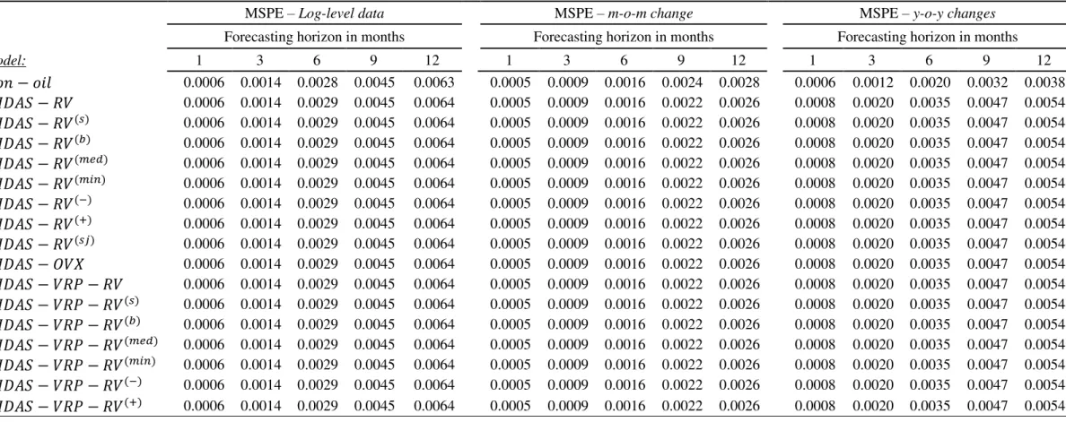
We start with the conditional forecasts of CPI, based on the modelling of the m-o-m
CPI changes, which are shown in Table 1. We can immediately understand there is no differentiation in terms of forecasting performance among the competing MIDAS models, which suggests that there is not a unique model specification that stands out. More importantly, though, we notice that the inclusion of the oil price forecasts (irrespectively of the oil price MIDAS model) as macroeconomic assumptions for core inflation prediction, does not provide any predictive gains since the non-oil model is constantly included in the set of the best models, according to the MCS test, across all forecasting horizons6.
[TABLE 1 HERE]
Such findings do not offer support to the views expressed by Natal (2012) that price stability is influenced by oil price fluctuations, especially in the short-run. By contrast, they provide support to the findings reported by Hooker (2002), Blanchard and Gali (2009) and Bachmeier and Cha (2011) who maintain that there is diminishing importance of oil prices on inflation rates. We should note, though, that none of these studies have assessed the impact of oil prices on inflation rates in a framework similar to ours.
Such diminishing importance of oil prices on inflation rates could be explained by the efficient energy use that has improved over the last decades, suggesting that oil prices should not matter recently as they used to in the past. Another potential explanation is provided by
Blanchard and Gali (2007) who opine that the flexibility of the labour market, as well as, the improved tools that are at the disposal of the monetary authorities have contributed to the decreased importance of oil prices on inflation rates.
Next, we consider the conditional forecasts of the industrial production index. The results are shown in Table 2.
[TABLE 2 HERE]
Similarly, with the results from Table 1, we show that the oil price forecasts do not seem capable of generated prediction gains relatively to the non-oil model. The MCS test inform us that the non-oil model is included in the set of the best performing models for all horizon up to 9-months ahead. Nevertheless, the results for the 12-months ahead horizon suggest that the conditional forecasts of the industrial production index that incorporate the oil prices forecasts based on OVX and the VRP of the two semi-variances (i.e. 𝑀𝐼𝐷𝐴𝑆 − 𝑂𝑉𝑋,
𝑀𝐼𝐷𝐴𝑆 − 𝑉𝑅𝑃 − 𝑅𝑉(−), 𝑀𝐼𝐷𝐴𝑆 − 𝑉𝑅𝑃 − 𝑅𝑉(+)) are the only ones that belong to the set of
the best predictive models. Despite the latter, we cannot support the view that oil price forecasts are particularly useful for industrial production predictions. Once again, our findings cannot offer support to Elder and Serletis (2010) who maintain that higher oil prices (and in particular the uncertainty surrounding them) have adverse impact on industrial production, especially after the mid-1970s.
The final macroeconomic indicator that we use is the purchasing price index, with the results being presented in Table 3.
[TABLE 3 HERE]
In the case of the PPI conditional forecasts, based on the modelling of the m-o-m PPI changes, the empirical findings from the conditional forecasts differ significantly relatively to the results already discussed for the core inflation and industrial production. More specifically, we observe that apart from the 1-month ahead horizon, the oil price forecasts generate significant forecasting gains (up to 48% relative to the non-oil model). Even more, we observe that the models that are constantly included in the set of the best performing models are primarily those with the VRP (and especially the 𝑀𝐼𝐷𝐴𝑆 − 𝑉𝑅𝑃 − 𝑅𝑉, 𝑀𝐼𝐷𝐴𝑆 − 𝑉𝑅𝑃 −
𝑅𝑉(𝑠)).
It is rather interesting, though, that despite the predictive power of oil prices on the purchasing price index, we cannot observe any such effects on the industrial production index or the inflation rate. At first, this may seem as a rather puzzling result; however, some plausible explanations are offered here. As far as the differentiating results between industrial production
and PPI are concerned, these may be justified by the fact that the former measures output units, whereas the latter shows cost prices. Oil prices are anticipated to influence production costs (hence the PPI index) and not necessarily the level of output. Furthermore, the finding that oil price forecasts can provide predictive information to the PPI index but not the CPI could be also explained by the fact that there is a shift in the weight of services in the US CPI calculation. More specifically, we observed an increasing weight of services over the last decades, reducing the importance of production goods (where many of them are oil-users) in the CPI7. This latter argument further justifies the lack of predictive gains from oil price forecasts to core inflation predictions.
5. Additional monetary policy indicators
In Section 4 we established that oil price forecasts, as macroeconomic assumptions for inflation predictions, are not economically useful. Thus, for robustness purposes we use oil price forecasts to predict two additional monetary policy related instruments, namely, the 5-year break-even inflation rate (𝐵𝐸𝐼𝑅𝑡), as well as, the monetary policy uncertainty index (𝑀𝑃𝑈𝑡). The choice of the former stems from the fact that it is one of the best indicators that captures inflation expectations (Ciccarelli and Garcia, 2009) and thus, its prediction is of major importance for policy makers. Inflation expectations are critical in evaluating (i) how effective the central bank communication is, and (ii) the predictions of real inflation. Thus, despite the fact the oil price forecasts may not be economically useful for inflation predictions, their importance may be manifested via their predictive power on inflation expectations.
As for the monetary policy uncertainty index, there is a recent literature that links oil prices with economic policy uncertainty (Antonakakis et al., 2014; Kang et al., 2017; Degiannakis and Filis, 2019), however, none of these papers assessed the economic usefulness of oil price forecasts on the predictability of the MPU index.
The monthly data for the US BEIR is obtained from the Federal Reserve of St. Luis (Federal Reserve Economic Data), whereas the data for the MPU is obtained from Baker et al.
(2016).
Similarly to the frameworks we used in Section 4, we estimate the following equation to generate conditional forecasts for both 𝐵𝐸𝐼𝑅𝑡 and 𝑀𝑃𝑈𝑡, based on oil price forecasts:
7 Please see a report from the Federal Reserve Bank of St. Louis on this issue: fredblog.stlouisfed.org/2018/11/ does-oil-drive-inflation/
𝑤𝑚,𝑡+ℎ = 𝑎 + ∑ 𝛽𝑖𝑤𝑡+ℎ−𝑖 𝐼 𝑖=1 + ∑ 𝛿𝑖𝛥(𝑂𝑖𝑙𝑚,𝑡+ℎ−𝑖|𝑡) 𝐼 𝑖=0 + 𝑒𝑡+ℎ (16)
where, 𝑤𝑚,𝑡+ℎ denotes either the 𝐵𝐸𝐼𝑅𝑡 or 𝑀𝑃𝑈𝑡 forecast at month 𝑡 + ℎ, 𝑂𝑖𝑙𝑚,𝑡+ℎ|𝑡 denotes the oil price prediction at month 𝑡 + ℎ given the information available at month 𝑡, and
𝑒𝑡~𝑁(0, 𝜎𝑒2) is the error term. For robustness purposes, we estimate eq.(16) for 𝑤𝑡 denoting
the log level of the 𝑀𝑃𝑈𝑡 index, as well as, its m-o-m and y-o-y changes8.
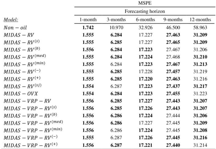
The results for the BEIR and MPU conditional forecasts are shown in Table 4. Our findings for BEIR are both important and interesting, as they show that oil price forecasts are economically useful for BEIR predictions, especially in the medium- and long-term horizons (i.e. 6-month up to 12 months ahead horizons). More specifically, the MCS test suggests that the non-oil model is only included in the set of the best performing models for the first two horizons. By contrast, the models that constantly outperform all others are the ones based on the intraday realised volatility measures, rather than the ones with the variance risk premiums or the implied volatility index (with the only exception being the
𝑀𝐼𝐷𝐴𝑆 − 𝑅𝑉(+) and 𝑀𝐼𝐷𝐴𝑆 − 𝑉𝑅𝑃 − 𝑅𝑉(−) models).
This might be another puzzling finding given that oil price forecasts do no provide gains for inflation predictions. Such finding may indicate that a monetary authority is not capable to offset oil price fluctuations in the medium-run (5 years ahead as we consider the 5-year BEIR), which could further suggest that inflation expectations are not well anchored to the long-run inflation target.
However, another plausible explanation here could be found to the alternative interpretation of the market-based measure of inflation expectations that is used in this paper, i.e. BEIR. Possibly what we observe here is that impact of oil price forecasts on the prediction of investors’ required return premiums for inflation risk and liquidity to their investments. Such link may not be far from reality given that in the last two decades we observe the increased financialisation of the oil market (see, for instance, Tang and Xiong, 2013; Degiannakis and Filis, 2017; Le Pen and Sévi, 2018), and especially of the WTI crude. Hence, we further document that oil price forecasts may not be useful for monetary authorities.
The latter argument is further supported by the results we obtain from the MPU conditional forecasts. We note that there is not a single specification that generates superior
8𝐵𝐸𝐼𝑅
conditional forecasts for the MPU index. Even more, we note that none of the MIDAS models is capable of enhancing the predictive accuracy of the non-oil models.
[TABLE 4 HERE]
6. Alternative oil price forecasting frameworks
So far, we have convincingly shown that oil price forecasts could be economically useful for policy makers, although this depends on the macroeconomic variable and the most appropriate transformation of the predicted series. To provide further robustness of our results, related to the use of the MIDAS model this time, we repeat the same conditional forecasts for the five different macroeconomic indicators, using as oil price assumptions the forecasts that have been generated by Kilian’s and co-authors VAR and Bayesian VAR (BVAR) models (see, for instance, Baumeister and Kilian, 2012, 2014, 2015 for the technical details). The results are shown in Table 5.
[TABLE 5 HERE]
In short, we observe that neither the VAR or the BVAR models can offer any improved predictive gains relatively to our MIDAS specifications. In fact, in many cases, the VAR and BVAR models are not included in the set of the best performing models, as assessed by the MCS test. These results strengthen our initial findings.
7. Conclusion
It is rather interesting that there is a vast literature supporting the view that oil price forecasts are important for a number of stakeholders, with the monetary authorities being among the key ones. Despite the improvements in oil price forecasting frameworks, the related literature has neglected to assess the economic usefulness of such forecasts. Such observation is even more striking since Alquist et al. (2013) and Kilian and Vigfusson (2017) put forward the arguments that oil price forecasts should have the potential to improve the forecasts for an array of macroeconomic variables and that modelling frameworks for oil prices should be ranked according to their conditional performance relatively to a macroeconomic variable.
Thus, adding to this important line of research, the aim of this study is to evaluate the economic usefulness of oil price forecasts by means of conditional forecasting of macroeconomic indicators. In particular, our main focus is on three core macroeconomic indicators that policy makers are forecasting, using assumptions about the future path of the oil prices. The chosen indicators are the core inflation rate, industrial production and purchasing
price index. In our framework we consider the oil price forecasts as our oil price assumptions in the conditional forecasting framework.
To do so, we initially forecast oil prices using a MIDAS model, where we model the future monthly crude oil prices based on high-frequency information obtained by different measures of oil price volatility and low-frequency oil price fundamentals. Subsequently, we use regression-based models for our conditional forecasts which are augmented with the oil price forecasts. As our naïve model we consider a regression-based model that does not contain the information from the oil price forecasts, which we name as non-oil model.
Our findings show that there is not a specific model that provides the higher predictive accuracy for the conditional forecasts of core inflation and industrial production. Even more, the mixed frequency models cannot provide predictive gains for these two macroeconomic indicators relatively to the non-oil model. By contrast, oil price forecasts generate significant forecasting gains (up to 48% relative to the non-oil model) for the PPI, while the MIDAS models that generate this superior predictive performance are primarily those that consider the variance risk premiums as their high-frequency predictors.
We further proceed with conditional forecasts for the break-even inflation (which approximates inflation expectations) and for an index of monetary policy uncertainty. These results suggest that on one hand, there is not a single MIDAS model that stands out as the best oil price forecasting model and on the other hand, none of the oil price forecasts can provide predictive information that is useful for the monetary authorities. To test further the robustness of our findings, we proceed with the oil price forecasts using other state-of-the-art forecasting frameworks, namely, VAR and Bayesian VAR models. The results show that oil price forecasts based on VAR and Bayesian VAR models cannot provide better conditional forecasts compared to the MIDAS specifications.
Overall, these findings suggest that there is diminishing importance of oil price forecasts for macroeconomic projections and for policy formulation of the monetary authorities. We offer an array of arguments as to why this might be the case. First, the improved energy efficiency along with the contemporary monetary policy tools could explain the decoupling between inflation rates and oil price fluctuations. Even more, the fact that in the US we observe an increase in the weight of services in the CPI calculation could explain the relative unimportance of oil price forecasts. On the other hand, the lack of predictive power of oil price forecasts on industrial production conditional forecasts could be explained by the fact that the former may impact production costs (i.e. the overall price of production inputs) but not the level of production output.
By contrast, the fact that our MIDAS models offer significant predictive gains for the conditional forecasts of inflation expectations could suggest that latter are not well anchored to the long-run inflation target. Nevertheless, given the lack of predictive gains that our models have on core inflation rate, we subscribe to the belief that an alternative explanation could be in place. In particular BEIR could reflect investors’ required return premiums for inflation risk and liquidity to their investments. Hence, the fact that oil price forecasts can improve the conditional forecasts for BEIR could constitute evidence of increased linkage between the bond and the oil market, which further suggests that the oil market is indeed financialised.
Overall, our findings do not argue against the usefulness of oil price forecasts. Rather, they tend to point out that such forecasts may not be useful for policy making purposes, whereas given the evidence provided by the recent literature, they may be more useful for investment purposes, possibly due to the market’s increased financialisation process.
Given the interesting findings presented in this study, it is important to expand this approach for the evaluation of oil price forecasts based on their economic usefulness to other countries or regions, which could be separated between industrial and post-industrial, as well as, net oil-importers and net-oil exporters.
References
Aguiar‐Conraria, L.U.Í.S. & Wen, Y. (2007). Understanding the large negative impact of oil shocks. Journal of Money, Credit and Banking, 39(4), 925-944.
Alquist, R. & Kilian, L. (2010). What do we learn from the price of crude oil futures?. Journal of Applied econometrics, 25(4), 539-573.
Alquist, R., Kilian, L. & Vigfusson, R.J. (2013). Forecasting the price of oil. Handbook of Economic Forecasting, 2, 427-507.
Andersen, T. G. & Bollerslev, T. (1998). Answering the skeptics: Yes, standard volatility models do provide accurate forecasts. International Economic Review, 885-905.
Andersen, T., Dobrev, D. & Schaumburg, E. (2012). Jump-Robust Volatility Estimation Using Nearest Neighbor Truncation. Journal of Econometrics, 169(1), 75-93.
Andreou, E., Ghysels, E. & Kourtellos, A. (2010). Regression models with mixed sampling frequencies. Journal of Econometrics, 158(2), 246-261.
Andreou, E., Ghysels, E. & Kourtellos, A. (2013). Should macroeconomic forecasters use daily financial data and how? Journal of Business & Economic Statistics, 31(2), 240-251.
Antonakakis, N., Chatziantoniou, I. & Filis, G. (2014). Dynamic spillovers of oil price shocks and economic policy uncertainty. Energy Economics, 44, 433-447.
Bachmeier, L. J. & Cha, I. (2011). Why don’t oil shocks cause inflation? Evidence from disaggregate inflation data. Journal of Money, Credit and Banking, 43(6), 1165-1183.
Backus, D. K. & Crucini, M. J. (2000). Oil prices and the terms of trade. Journal of International Economics, 50(1), 185-213.
Baker, S. R., Bloom, N. & Davis, S. J. (2016). Measuring economic policy uncertainty. The Quarterly Journal of Economics, 131(4), 1593-1636.
Bańbura, M., Giannone, D. & Lenza, M. (2015). Conditional forecasts and scenario analysis with vector autoregressions for large cross-sections. International Journal of Forecasting,
31(3), 739-756.
Barnato, K. (2016).Here’s the key challenge Draghi will face at this week’s ECB meeting, CNBC, 30th May, http://www.cnbc.com/2016/05/30/heres-the-key-challenge-draghi-will-face-at-this-weeks-ecb-meeting.html.
Barndorff-Nielsen, O. & Shephard, N. (2004). Power and bipower variation with stochastic volatility and jumps. Journal of Financial Econometrics, 2(1), 1-37.
Barndorff-Nielsen, O. & Shephard, N. (2006). Econometrics of Testing for Jumps in Financial Economics Using Bipower Variation. Journal of Financial Econometrics, 4, 1-30.
Baumeister, C., Guérin, P. & Kilian, L. (2015). Do high-frequency financial data help forecast oil prices? The MIDAS touch at work. International Journal of Forecasting, 31(2), 238-252.
Baumeister, C. & Kilian, L. (2012). Real-time forecasts of the real price of oil. Journal of Business & Economic Statistics, 30(2), 326-336.
Baumeister, C. & Kilian, L. (2014). What central bankers need to know about forecasting oil prices. International Economic Review, 55(3), 869-889.
Baumeister, C. & Kilian, L. (2015). Forecasting the real price of oil in a changing world: a forecast combination approach. Journal of Business & Economic Statistics, 33(3), 338-351.
Baumeister, C., Kilian, L. & Lee, T.K. (2014). Are there gains from pooling real-time oil price forecasts? Energy Economics, 46, S33-S43.
Baumeister, C., Kilian, L. & Zhou, X. (2018). Are product spreads useful for forecasting? An empirical evaluation of the Verleger hypothesis. Macroeconomic Dynamics, 22, 562-580.
Blair, B.J., Poon, S.H. and Taylor, S.J. (2001). Forecasting S&P100 Volatility: the Incremental Information Content of Implied Volatilities and High Frequency Returns.
Journal of Econometrics, 105, 5 -26.
Blanchard, O. & Gali, J. (2009). The Macroeconomic Effects of Oil Shocks: Why Are the 2000s So Different from the 1970’s?. In: International Dimensions of Monetary Policy, edited by Jordi Gali and Mark Gertler, pp. 373–428. Chicago: University of Chicago Press.
Blas, J. & Kennedy, S. (2016). For Once, Low Oil Prices May Be a Problem for World's Economy, Bloomberg, 2nd February, https://www.bloomberg.com/news/articles/2016-02-02/for-once-low-oil-prices-may-be-a-problem-for-world-s-economy.
Bollerslev, T., Tauchen, G. & Zhou, H. (2009). Expected stock returns and variance risk premia. The Review of Financial Studies, 22(11), 4463-4492.
Barndorff-Nielsen, O., Kinnebrock, S. & Shephard, N. (2010). Measuring downside risk – Realised semivariance. In: T. Bollerslev, J. Russell and M. Watson (eds) Volatility and Time Series Econometrics: Essays in Honor of Robert F. Engle. Oxford University Press.
Carr, P. & Wu, L. (2008). Variance risk premiums. The Review of Financial Studies, 22(3), 1311-1341.
Ciccarelli, M. & Garcia, J.A. (2009). What drives euro area break-even inflation rates?, European Central Bank working paper series, No. 996.
Clark, T.E. & West, K.D. (2007). Approximately normal tests for equal predictive accuracy in nested models. Journal of Econometrics, 138, 291–311.
Coibion, O. & Gorodnichencko, Y. (2015). Is the Phillips curve alive and well after all? Inflation expectation and the missing disinflation. American Economic Journal: Macroeconomics. 7 (1), 197–232.
Coimbra, C. & Esteves, P.S. (2004). Oil price assumptions in macroeconomic forecasts: should we follow futures market expectations? OPEC review, 28(2), 87-106.
Degiannakis, S. & Filis, G. (2018). Forecasting oil prices: High-frequency financial data are indeed useful. Energy Economics, 76, 388-402.
Degiannakis, S., Filis, G., & Arora, V. (2018a). Oil prices and stock markets: a review of the theory and empirical evidence. The Energy Journal, 39(5), 85-130.
Degiannakis, S. & Filis, G. (2019). Forecasting European economic policy uncertainty.
Scottish Journal of Political Economy, 66(1), 94-114.
Degiannakis, S., Filis, G. & Hassani, H. (2018b). Forecasting global stock market implied volatility indices. Journal of Empirical Finance, 46, 111-129.
ECB (2015). Economic Bulletin, Issue 4, European Central Bank. https://www.ecb.europa.eu/pub/pdf/other/art03_eb201504.en.pdf?cf0bb5d2a75e31d43e38 b3c5d5540273.
ECB (2016a). Economic Bulletin, Issue 4, European Central Bank. https://www.ecb.europa.eu/pub/pdf/other/eb201604_focus01.en.pdf?48284774d83e30563 e8f5c9a50cd0ea2.
ECB (2016b). A guide to the Eurosystem/ECB staff macroeconomic projection exercises,
European Central Bank,
https://www.ecb.europa.eu/pub/pdf/other/staffprojectionsguide201607.en.pdf.
Elder, J. & Serletis, A. (2010). Oil price uncertainty. Journal of Money, Credit and Banking,
42(6), 1137-1159.
Gelos, G. & Ustyugova, Y. (2017). Inflation responses to commodity price shocks–How and why do countries differ. Journal of International Money and Finance. 72, 28–47.
Ghysels, E., Santa-Clara, P. & Valkanov, R. (2006). Predicting volatility: getting the most out of return data sampled at different frequencies. Journal of Econometrics, 131(1-2), 59-95.
Giannone, D., Lenza, M., Momferatoud, D. & Onorante, L. (2014). Short-term inflation projections: A Bayesian vector autoregressive approach. International Journal of Forecasting. 30, 635-644.
Güntner, J.H. & Linsbauer, K. (2018). The effects of oil supply and demand shocks on US consumer Sentiment. Journal of Money, Credit and Banking, 50(7), 1617-1644.
Hamilton, J. D. (2008). Oil and the macroeconomy, The new Palgrave Dictionary of Economics. Blume (second ed.), Palgrave Macmillan.
Hansen, P.R. (2005). A test for superior predictive ability. Journal of Business & Economic Statistics, 23, 365–380.
Hansen, P.R. & Lunde, A. (2005). A Realized Variance for the Whole Day Based on Intermittent High-Frequency Data. Journal of Financial Econometrics, 3(4), 525-554.
Hooker, M. A. (2002). Are oil shocks inflationary? Asymmetric and nonlinear specifications versus changes in regime. Journal of Money, Credit, and Banking, 34(2), 540–561.
IMF (2016). World Economic Outlook – Too slow for too long, International Monetary Fund: Washington DC.
Jo, S. (2014). The effects of oil price uncertainty on global real economic activity. Journal of Money, Credit and Banking, 46(6), 1113-1135.
Kang, W., de Gracia, F.P. & Ratti, R.A. (2017). Oil price shocks, policy uncertainty, and stock returns of oil and gas corporations. Journal of International Money and Finance, 70, 344-359.
Kilian, L., Rebucci, A. & Spatafora, N. (2009). Oil shocks and external balances. Journal of International Economics, 77(2), 181-194.
Kilian, L. & Vigfusson, R.J. (2013). Do oil prices help forecast US real GDP? The role of nonlinearities and asymmetries. Journal of Business & Economic Statistics, 31(1), 78-93.
Kilian, L. & Vigfusson, R.J. (2017). The role of oil price shocks in causing US recessions.
Journal of Money, Credit and Banking, 49(8), 1747-1776.
Koopman, S.J., Jungbacker, B. and Hol, E. (2005). Forecasting daily variability of the S&P 100 stock index using historical, realised and implied volatility measurements. Journal of Empirical Finance, 12(3), 445-475.
Le Pen, Y., & Sévi, B. (2018). Futures trading and the excess co-movement of commodity prices. Review of Finance, 22(1), 381-418.
Marcellino, M., Stock, J.H. & Watson, M.W. (2003). Macroeconomic forecasting in the euro area: Country specific versus area-wide information. European Economic Review, 47(1), 1-18.
Martens, M. (2002). Measuring and forecasting S&P 500 index‐futures volatility using high‐ frequency data. Journal of Futures Markets: Futures, Options, and Other Derivative Products, 22(6), 497-518.
Natal, J. (2012). Monetary policy response to oil price shocks. Journal of Money, Credit and Banking, 44(1), 53-101.
Naser, H. (2016). Estimating and forecasting the real prices of crude oil: A data rich model using a dynamic model averaging (DMA) approach. Energy Economics, 56, 75-87.
Patton, A.J. & Sheppard, K. (2015). Good volatility, bad volatility: signed jumps and the persistence of volatility. The Review of Economics and Statistics, 97(3), 683-697.
Prokopczuk, M., Symeonidis, L. & Simen, C.W. (2017). Variance risk in commodity markets. Journal of Banking & Finance, 81, 136-149.
Ravazzolo, F. & Rothman, P. (2013). Oil and US GDP: A Real‐Time Out‐of‐Sample Examination. Journal of Money, Credit and Banking, 45(2‐3), 449-463.
Renou-Maissant, P. (2019). Is oil price still driving inflation?. The Energy Journal, 40(6), 199-219.
Tang, K., & Xiong, W. (2012). Index investment and the financialization of commodities.
Financial Analysts Journal, 68(6), 54-74.
Tee, C. W. & Ting, C. (2017). Variance risk premiums of commodity ETFs. Journal of Futures Markets, 37(5), 452-472.
Theodosiou, M. and Zikes, F. (2009). A comprehensive comparison of alternative tests for jumps in asset prices. Imperial College London.
White, H. (2000). A reality check for data snooping. Econometrica, 68, 1097–1126.
Zhang, Y., Ma, F., Shi, B. & Huang, D. (2018). Forecasting the prices of crude oil: An iterated combination approach. Energy Economics, 70, 472-483.
FIGURES
Figure 1. WTI oil prices, oil price volatility and variance risk premium
20 40 60 80 100 120 10 11 12 13 14 15 16 17 WTI price 0 20 40 60 80 100 120 10 11 12 13 14 15 16 17 WTI ScaledRV 0 20 40 60 80 100 10 11 12 13 14 15 16 17 WTI RSV+ 10 20 30 40 50 60 70 80 10 11 12 13 14 15 16 17 OVX -40 -20 0 20 40 60 10 11 12 13 14 15 16 17 WTI VRP (RSV-) -60 -40 -20 0 20 40 60 10 11 12 13 14 15 16 17 WTI VRP (MinRV)
Figure 2. WTI oil prices, oil price volatility and variance risk premium for a random month 86 88 90 92 94 96 98 1 2 3 6 7 8 9 10 13 14 15 16 17 20 21 22 23 24 27 28 29 30 M8 WTI price 10 15 20 25 30 35 1 2 3 6 7 8 9 10 13 14 15 16 17 20 21 22 23 24 27 28 29 30 M8 WTI ScaledRV 8 12 16 20 24 28 32 1 2 3 6 7 8 9 10 13 14 15 16 17 20 21 22 23 24 27 28 29 30 M8 WTI RSV+ 29 30 31 32 33 34 35 1 2 3 6 7 8 9 10 13 14 15 16 17 20 21 22 23 24 27 28 29 30 M8 OVX 0 5 10 15 20 25 1 2 3 6 7 8 9 10 13 14 15 16 17 20 21 22 23 24 27 28 29 30 M8 WTI VRP (RSV-) -5 0 5 10 15 20 1 2 3 6 7 8 9 10 13 14 15 16 17 20 21 22 23 24 27 28 29 30 M8 WTI VRP (MinRV)
TABLES
Table 1: Oil price forecast evaluation based on conditional forecasts of core CPI based on m-o-m changes. Evaluation period: 2014.12-2017.10.
MSPE Forecasting horizon
Model: 1-month 3-months 6-months 9-months 12-months
𝑁𝑜𝑛 − 𝑜𝑖𝑙 0.0005 0.0009 0.0016 0.0024 0.0028 𝑀𝐼𝐷𝐴𝑆 − 𝑅𝑉 0.0005 0.0009 0.0016 0.0022 0.0026 𝑀𝐼𝐷𝐴𝑆 − 𝑅𝑉(𝑠) 0.0005 0.0009 0.0016 0.0022 0.0026 𝑀𝐼𝐷𝐴𝑆 − 𝑅𝑉(𝑏) 0.0005 0.0009 0.0016 0.0022 0.0026 𝑀𝐼𝐷𝐴𝑆 − 𝑅𝑉(𝑚𝑒𝑑) 0.0005 0.0009 0.0016 0.0022 0.0026 𝑀𝐼𝐷𝐴𝑆 − 𝑅𝑉(𝑚𝑖𝑛) 0.0005 0.0009 0.0016 0.0022 0.0026 𝑀𝐼𝐷𝐴𝑆 − 𝑅𝑉(−) 0.0005 0.0009 0.0016 0.0022 0.0026 𝑀𝐼𝐷𝐴𝑆 − 𝑅𝑉(+) 0.0005 0.0009 0.0016 0.0022 0.0026 𝑀𝐼𝐷𝐴𝑆 − 𝑅𝑉(𝑠𝑗) 0.0005 0.0009 0.0016 0.0022 0.0026 𝑀𝐼𝐷𝐴𝑆 − 𝑂𝑉𝑋 0.0005 0.0009 0.0016 0.0022 0.0026 𝑀𝐼𝐷𝐴𝑆 − 𝑉𝑅𝑃 − 𝑅𝑉 0.0005 0.0009 0.0016 0.0022 0.0026 𝑀𝐼𝐷𝐴𝑆 − 𝑉𝑅𝑃 − 𝑅𝑉(𝑠) 0.0005 0.0009 0.0016 0.0022 0.0026 𝑀𝐼𝐷𝐴𝑆 − 𝑉𝑅𝑃 − 𝑅𝑉(𝑏) 0.0005 0.0009 0.0016 0.0022 0.0026 𝑀𝐼𝐷𝐴𝑆 − 𝑉𝑅𝑃 − 𝑅𝑉(𝑚𝑒𝑑) 0.0005 0.0009 0.0016 0.0022 0.0026 𝑀𝐼𝐷𝐴𝑆 − 𝑉𝑅𝑃 − 𝑅𝑉(𝑚𝑖𝑛) 0.0005 0.0009 0.0016 0.0022 0.0026 𝑀𝐼𝐷𝐴𝑆 − 𝑉𝑅𝑃 − 𝑅𝑉(−) 0.0005 0.0009 0.0016 0.0022 0.0026 𝑀𝐼𝐷𝐴𝑆 − 𝑉𝑅𝑃 − 𝑅𝑉(+) 0.0005 0.0009 0.0016 0.0022 0.0026
Note: Bold face indicates that the model is among the set of the best performing models according to the Model Confidence Set (MCS) test.
Table 2: Oil price forecast evaluation based on conditional forecasts of IP, based on the log-level data. Evaluation period: 2014.12-2017.10.
MSPE Forecasting horizon
Model: 1-month 3-months 6-months 9-months 12-months
𝑁𝑜𝑛 − 𝑜𝑖𝑙 0.2526 1.1190 2.7032 5.5700 9.3322 𝑀𝐼𝐷𝐴𝑆 − 𝑅𝑉 0.2472 0.9284 2.2922 4.4508 7.5352 𝑀𝐼𝐷𝐴𝑆 − 𝑅𝑉(𝑠) 0.2472 0.9284 2.2924 4.4514 7.5353 𝑀𝐼𝐷𝐴𝑆 − 𝑅𝑉(𝑏) 0.2472 0.9284 2.2922 4.4510 7.5344 𝑀𝐼𝐷𝐴𝑆 − 𝑅𝑉(𝑚𝑒𝑑) 0.2472 0.9284 2.2918 4.4507 7.5357 𝑀𝐼𝐷𝐴𝑆 − 𝑅𝑉(𝑚𝑖𝑛) 0.2472 0.9284 2.2922 4.4508 7.5348 𝑀𝐼𝐷𝐴𝑆 − 𝑅𝑉(−) 0.2472 0.9284 2.2928 4.4502 7.5380 𝑀𝐼𝐷𝐴𝑆 − 𝑅𝑉(+) 0.2473 0.9283 2.2916 4.4514 7.5332 𝑀𝐼𝐷𝐴𝑆 − 𝑅𝑉(𝑠𝑗) 0.2472 0.9286 2.2926 4.4510 7.5360 𝑀𝐼𝐷𝐴𝑆 − 𝑂𝑉𝑋 0.2471 0.9283 2.2923 4.4502 7.5342 𝑀𝐼𝐷𝐴𝑆 − 𝑉𝑅𝑃 − 𝑅𝑉 0.2472 0.9286 2.2925 4.4498 7.5337 𝑀𝐼𝐷𝐴𝑆 − 𝑉𝑅𝑃 − 𝑅𝑉(𝑠) 0.2472 0.9286 2.2927 4.4504 7.5341 𝑀𝐼𝐷𝐴𝑆 − 𝑉𝑅𝑃 − 𝑅𝑉(𝑏) 0.2472 0.9286 2.2922 4.4501 7.5327 𝑀𝐼𝐷𝐴𝑆 − 𝑉𝑅𝑃 − 𝑅𝑉(𝑚𝑒𝑑) 0.2472 0.9285 2.2921 4.4499 7.5353 𝑀𝐼𝐷𝐴𝑆 − 𝑉𝑅𝑃 − 𝑅𝑉(𝑚𝑖𝑛) 0.2472 0.9286 2.2923 4.4504 7.5347 𝑀𝐼𝐷𝐴𝑆 − 𝑉𝑅𝑃 − 𝑅𝑉(−) 0.2472 0.9286 2.2932 4.4503 7.5331 𝑀𝐼𝐷𝐴𝑆 − 𝑉𝑅𝑃 − 𝑅𝑉(+) 0.2472 0.9287 2.2918 4.4500 7.5291
Note: Bold face indicates that the model is among the set of the best performing models according to the Model Confidence Set (MCS) test.