Demand Forecasting Using Bayesian Experiment with Non-homogenous Poisson Process Model

International Journal of Operations Research Vol. 2, No. 1, 21−29 (2005)

Demand Forecasting Using Bayesian Experiment with

Non-homogenous Poisson Process Model

Hung-Ju Wang

1, 2

_{, Chen-Fu Chien}

1,*

_{, and Ching-Fang Liu}

1

1 _{Department of Industrial Engineering and Engineering Management, National Tsing Hua University, Hsinchu 300,}

Taiwan. R.O.C.

2 _{Ministry of Economics, Taipei 100, Taiwan. R.O.C}

Abstract

⎯

This study presents a novel mathematical model using Bayesian model for demand forecasting with

non-homogenous Poisson process model. This study aims to construct a framework to minimize the overproduction and underproduction costs by using the time-dependent uncertainty of accumulative demand curve. Specific models were derived as the fundamentals of this approach. Furthermore, this study also proposed a method to evaluate demand forecasting using Bayesian experiment with non-homogenous Poisson process model.

Keywords

⎯

Demand forecasting, Poisson process, Bayesian, Mathematical model, Decision analysis

*_{Corresponding author’s email: [email protected]}

1. INTRODUCTION

Successful performance of revenue management systems heavily relies on forecasting and optimization (Rajopadhye et al., 1999). Based on the historical demand data, researchers have applied time series or other statistical analysis methods for demand forecast. For example, Holt-Winters exponential smoothing model for optimal forecasting is applied for short-term forecasts for series of sales data or levels of demand for goods (Segura and Vercher, 2001). Rather than using single forecasting method, Witt and Witt (1995) proposed auto-regression, exponential smoothing, and econometrics for forecasting tourism demand. With aggregate slack control or multistage production control, the master planning procedure with the variance of production and inventory levels can avoid the unrestrained growth of inventory and the uncontrollable consumption of capacity (Bartezzaghi and Verganti, 1995, Hirakawa, 1996).

Alternatively, this study aims to construct a framework to minimize the overproduction and underproduction costs by using the time-dependent uncertainty of accumulative demand curve in which some properties of the Poisson process are introduced and the relation between the Poisson process and Bayes’ theory is identified. Due to the stochastic characteristics of the future capacity needs by input and output process (Lattimore and Baker, 1997), the Poisson process and Bayes’ theory (Cinlar, 1975) are adopted herein. This approach is different from the Bayesian analysis of the Muth model and mixed Markov with latent class model e.g., Urban et al. (1996), Goulias (1999). Because this mathematical model is derived from the past sales experiment, the technology of pre-market forecasting of new product may not be suitable by lacking of the historical data (Gavirneni et al., 1998). Furthermore, this

study also proposed a method to evaluate demand forecasting using Bayesian experiment with non-homogenous Poisson process model. These indices of evaluation are essential in revenue management.

The rest of this paper is organized as follows. Section 2 establishes the theoretical foundation and describes the proposed mathematical models. Section 3 introduces the evaluation process that considers overproduction and underproduction costs to assess the accumulative demand curve and its uncertainty. Concluding remarks are finally made in section 4, including the merits and limitations of the proposed procedure.

2. MATHEMATICAL MODEL

The following terminology and notations are generally used in this study.

( , )n t

λ : the event rate for each n event occurs in t period.

( )n

λ : the average of random event rate.

( )

h t : the accumulative demand function of time t.

( )

c λ : constant of event rate.

( ) k

n t : volume of product nk at time t.

t: time period or time interval.

( | , ( , ))

P n t λ n t : a Poisson process presents the probability of product n’s demand at given time t and event

rateλ( , )n t .

( | , ( , ))

f t n λ n t : a conditional probability function of gamma distribution for time interval t given n andλ( , )n t .

Herein, the Poisson process is adopted for demand forecasting. Especially, the linkage between demand forecasting and inventory management can be applied in a model with condensed and compounded Poisson mixed over time (Boylan and Johnston, 1996). In the general model of Poisson process, researchers usually use the

OperationsResearch

constant event rate as the parameter of λ (Hogg and Tanis, 1983). Some gaps exist between the Poisson process and Bayes’ theory in terms of the event rate updated. That means the λ could be variable instead of constant parameter.

Theorem 1: If a specific event in a system occurs as a

Poisson experiment, the derived Bayesian model on the event rate will have the likelihood function as a Poisson distribution. That is,

0 0 1 _{( , )} 0 ( ) ( ) 0 1 ( , ) ( | , ( , )) ! 1 ( ) ( ) ! t t n t n d t n t n n h d t n d t P n t n t e n n h d t e n λ τ τ λ _{τ τ} λ τ τ λ λ τ τ − − ⎛ ⎞ ⎜ ⎟ _∫ ⎝ ⎠ = ⎛ ⎞ ⎜ ⎟ _∫ ⎝ ⎠ =

∫

∫

(1)

Proof: see Wang and Chien (2000).

In Theorem 1, the Poisson process and Bayes’ theory are related in terms of the randomness of event rate. The intuition of this conversion comes from the model in Drinking Water Company of Limburg (WML) who changes the constant production flow into optimization of the quantitative control Baker et al. (1998).

From the above theorem, we can infer that the posterior distribution of event rate is gamma distribution. For the randomness of event rate, we assume there is a demand curve with time dependent function h t( ) that affects the mean of that event rate. The non-homogenous Poisson process model can be applied to deal with the randomness of an event rate can combine the Poisson process and Bayes’ theory to solve the problem of time dependency on the event rate.

Theorem 2: If a specific event in a system occurs as a

Poisson experiment with the time dependent event rate, the derived Bayesian model will have the likelihood function as a Poisson distribution. That is,

( )

( ) 0 ( ) 0 1 _{( )} ( , , ( , )) ! t n t n c h d t c h d t f n t n t e n λ _{τ τ} λ τ τ λ − ⎡ ⎤ ⎢ ⎥ _∫ ⎣ ⎦ =

∫

(9)

Proof: see appendix 1.

Hence, Theorem 2 links the non-homogenous Poisson process and the Bayes’ theory. Then, the demand curve

( )

h t is the accumulative and the event rate λ( , )n t is equal to ( ) 1 t ( )

o

n h d t

λ ×

_∫

τ τ with the randomness of

( )n

λ which c

( )

λ =λ

( )

n in equation (9). From the properties of Poisson process, we know that the probability distribution of the random variable ni,

representing the number of products demand in a given time interval denoted by t.

Theorem 3: If concurrent specific events n1(t), n2(t),…, nm(t) in a system or component occur as its Poisson experiment respectively on the same event rate λ, the derived Bayesian model with maximum likelihood estimator (Cinlar, 1975) will satisfy

[ ]

( )

1 0 m k k t n E _m h d t λ τ τ = =

∑

∫

(11)

Proof: see appendix 2.

Theorem 3 specifies the relationship between the randomness event rate λ

( )

n and the accumulative demand h t( ) is of relevant concern.

Theorem 4: If concurrent specific events n1(t), n2(t),…, nm(t) in a system occur as its Poisson experiment respectively on the same event rate λ( , )n t , the derived Bayesian model with maximum likelihood estimator will satisfy 0 1 [ | , ] ( ) t n E n t h d t λ τ τ + = ∫ (13) and ₂ 0 1 ( | , ) ( ) t n Var n t h d t λ τ τ + = ⎛_∫ ⎞ ⎜ ⎟ ⎜ ⎟ ⎝ ⎠ (15)

Proof: see appendix 3.

Because the accumulative demand curve is a non-decreasing function as time goes by, the larger demand requirement implies a smaller uncertainty of event rate.

Theorem 5: Mentioned about average time case of

0

1t_{h( )d}

t

∫

τ τ  there is a saddle point in warning productivity

strategy with increasing ( )h t 

0 1 If ''( ) 0, ( ) ( ) ( ) 2 t t f t h d h t h t t τ τ ′ =

_∫

= − (17)

Proof: see appendix 4.

3. EVALUATION PROCESS

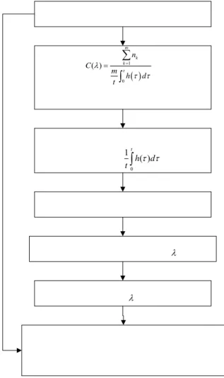
The above theorems and properties in the non-homogenous Poisson process can be applied to develop an evaluation process of demand forecasting as

shown in Figure 1. In this evaluation process, to collect demand curve based on historical data of similar products is the main processing of data analysis in the proposed framework (Lertpalangsunti and Chan, 1998).

As illustrated in Figure 1, the evaluation process consists of six steps.

Firstly, the historical demand data of a specific product or similar products with n1(t), n2(t), …, nm(t) at some

certain time are collected. Following the nature of a lumpy demand (Bartezzaghi et al., 1999), if this product is a new one, some similar products can be used to replace the average demand data n1(t), n2(t), …, nm(t). If the demand

data can not be collected, the accumulative sales data can also be used to substitute the average demand data, though the underproduction cost (Fisher and Raman, 1996) may be underestimated.

Secondly, the unbiased minimum variance estimator is used as the average demand data. There are some specific time points for collecting the average demand data. The unbiased minimum variance estimator uses the mean value of these data as the prediction of the accumulative curve at the selected time points. That is,

0 1 ( ) t h d t

∫

τ τ = 1 ( ) m k k=n t m

∑

is a point estimator of the average demand at time t.

Thirdly, the cubic spline technique in numerical analysis (Burden et al., 1985) is employed to smooth the average demand curve. Since only the data at some specific time points are derived in the second step, the continuous demand rate h t( ) can be derived, which is easier to derive the average demand curve by integration.

Fourthly, Theorem 4 is employed to obtain the mean and variance value of event rate λ for measuring the demand uncertainty. In particular,

2 0 1 ( | , ) 1t _{( )} n Var n t h d t λ τ τ + = ⎛ ⎞ ⎜ ⎟ ⎝

∫

⎠

implies a large uncertainty at the beginning of sales, if there is an idle time passed. The product strategy significantly affects the profit outcome at the beginning of sales and thus makes the product sales more uncertain of the beginning than some sales periods later after some sales period.

Fifthly, Theorem 2 is employed to evaluate the randomness of event rate λ after some sales periods. According to equation (17), the variance of the randomness in event rate λ is convergent with an increase of the accumulative demand.

Finally, reduced cost of demand uncertainty technology (Fisher and Raman, 1996) can be applied to minimize the overproduction and underproduction costs. When sales rate of h t( )is increasing and before reaching the saddle point of

0

1 t _{( )}

h d

t

∫

τ τ , we can expand our productivity by

the average demand curve and its randomness to derive the probabilities of overproduction and underproduction.

The expected value of overproduction cost can be derived from the product of discount cost in each product and its overproduced probability. Similarity, the expected value of underproduction cost can be derived from the product of shortage cost in each product and its underproductive probability. Moreover, the production plan and schedule can be evaluated by the total overproduction cost and underproduction cost during the sales periods.

There is a significant difference between this model and origin-destination (OD) demand prediction (Camus et al., 1997). Rather than using the time slice in OD demand matrices, this model provides an integral estimation at any time. Indeed, the product of λ×h t( ) is similar to the simplified formula in exponential smoothing models (Winter, 1960, Salem and Jacques, 1999). The feedback loop of evaluation process is the results refinement and validation in that framework.

( ) 1 0 ( ) m k k t n C m h d t λ τ τ = = ∑ ∫ 0 1 ( ) t h d t

∫

τ τ λ λ

Figure 1. Evaluation process of demand forecasting.

4. CONCLUDING REMARKS

This study derives mathematical models in demand forecasting and proposes a corresponding process for evaluating demand forecast. The proposed model can provide useful information such as variation of product demand at different times. With the uncertainty of accumulative demand curve being estimated, this method can be used to minimize the overproduction and

underproduction costs. Therefore, the proposed model can be used to evaluate the production plan and schedule based on the total production costs including overproduction and underproduction costs. The results for demand forecasting derived in this approach can be integrated with revenue management to maximize the revenue in light of the fixed discount cost, shortage cost, and stochastic average demand curve during a sales period.

Further study is needed to use empirical data for validating the practical viability of the proposed model.

ACKNOWLEDGEMENTS

This research is sponsored by National Science Council, Taiwan, R.O.C. (NSC 93-2213-E-007-008).

APPENDIX 1

Consider that there is a functional random variable λ( , )n t in a Poisson process such that

0

1 ( , )= ( )n t n th( )d

t

λ λ ×

∫

τ τ

with λ(n) is a random event rate and h(n) is a function of time t. Here, we use the average of random event rate to represent the parameter λ(n). Then, for each n event occurs in t period, we can get

0 0 ( ) 1 _{( , ) ( )} 0 0 1 _{( , ) ( )} 1 _{( )} ( | , ( , )) ! ! t t n n t t n n n d h d t t n d n h d t t P n t n t e e n n λ λ τ τ τ τ λ τ τ λ τ τ λ − − ⎛ ⎞ ⎛ ⎞ ⎜ ⎟ _∫ ⎜ ⎟ _∫ ⎝ ⎠ ⎝ ⎠ =

∫

=

∫

(1) In addition, let f t n( | , ( , ))λ n t be a conditional probability function of gamma distribution for time interval t given n and λ(n, t), where time t is a continuous variable Thus,

0 0 ( ) 1 _{( , ) ( )} 0 0 1 _{( , ) ( )} 1 _{( )} ( | , ( , )) = ! ! t t n n t t n n n d h d t t n d n h d t t f t n n t e e n n λ λ τ τ τ τ λ τ τ λ τ τ λ − − ⎛ ⎞ ⎛ ⎞ ⎜ ⎟ _∫ ⎜ ⎟ _∫ ⎝ ⎠ ⎝ ⎠ =

∫

∫

(2) On one hand, 0 ( , , ( , )) ( | , ( , )) ( , , ( , )) k f n t n t P n t n t f k t n t λ λ λ ∞ = =

∑

∵ ( , , ( , )) ( | , ( , )) ( , , ( , )) f n t λ n t P n t λ n t f k t λ n t ∴ =

∑

0 ( ) ( ) 0 0 ( , , ( , )) 1 ( ) ( ) ( , , ( , )) ! t n t n n h d t k f n t n t n h d t e f k t k t n λ _{τ τ} λ λ τ τ λ − ∞ = ⎛ ⎞ ⎜ ⎟ _∫ ⎝ ⎠ =

∫

∑

(3)

On the other hand,

0 ( , , ( , )) ( | , ( , )) ( , , ( , )) f n t n t f t n n t f n t n t dt λ λ λ ∞ =

∫

∵ 0 ( , , ( , )) ( | , ( , )) ( , , ( , )) f n t λ n t f t n λ n t ∞ f n t λ n t dt ∴ =

_∫

by (2), 0 ( ) ( ) 0 0 1 ( ) ( ) ( , , ( , )) ( , , ( )) ! t n t n n h d t n h d t f n t n t e f n t t dt n λ _{τ τ} λ τ τ λ − ∞ λ ⎛ ⎞ ⎜ ⎟ _∫ ⎝ ⎠ =

∫

_∫

(4)

From equation (4), we derive: 0 0 ( ) 1 _{( )} 0 0 1 ( ) _{( )} 0 0 ( ) ( ) ( , , ( , )) _{( , , ( , ))} ! ( ) ( ) ( ) ( , , ( , )) ! t t n t n n n _{h d} t n t n n n h d t n n h d t f n t n t _{e f n t n t dt} t n n n h t h d t e f n t n t dt n λ _{τ τ} λ _{τ τ} λ τ τ λ _λ λ τ τ λ λ + − ∞ − ∞ − ⎛ ⎞ ⎜ ⎟ _∫ ∂ _{⎝ ⎠} = − ∂ ⎛ ⎞ ⎜ ⎟ _∫ ⎝ ⎠ + −

∫

∫

∫

∫

0 0 n 1 ( ) 1 ( ) 0 0 n 1 ( ) 2 ( ) 0 0 0 1 ( ) ( ) ( ) ( , , ( , )) ! 1 ( ) ( ) ( ) ( , , ( , )) ! ( ) ( ) t t n t n n h d t n t t n n h d t n h t h d t e f n t n t dt n n h d h d t e f n t n t dt n nh t n t h λ _{τ τ} λ _{τ τ} τ τ λ λ τ τ τ τ λ τ + + − ∞ + + − ∞ ⎛ ⎞ ⎜ ⎟ _∫ ⎝ ⎠ ⎛ ⎞ ⎜ ⎟ _∫ ⎝ ⎠ + = − +

∫

∫

∫

∫

∫

2 0 0 ( ) ( ) ( ) ( ) ( , , ( , )) t t n n h t h d f n t n t t t d λ λ _{τ τ λ} τ ⎡ ⎤ ⎢ ⎥ ⎢ _{− +} ⎥ ⎢ ⎥ ⎢ ⎥ ⎢ ⎥ ⎣ ⎦

∫

∫

(5) Then,

[

]

0

[ ]

0 ( ) ln ( ) ( ) ln ( , , ( , )) ln t t n n h d h d t f n t n t t t t t t λ τ τ τ τ λ ⎡ ⎤ ⎡ ⎤ ∂ _{⎢ ⎥} ∂_{⎢ ⎥} ∂ _{⎣ ⎦} ∂ _{⎣ ⎦} = − − ∂ ∂ ∂ ∂

∫

∫

(6) Thus, 0 ( ) ( ) 0 1 ( , , ( , )) ( ) ( ) t n n t h d t n f n t n t n h d e t λ _{τ τ} λ =λ ⎛_⎜ τ τ⎞_⎟ − ∫ ⎝

∫

⎠ (7)

Compare the result of equation (7) and equation (3), we obtain:

0 0 ( ) _{( )} 0 0 ( ) ( ) 0 1 ( ) ( ) ( , , ( , )) ( , , ( , )) ! 1 ( ) ( ) ! t t n t n n _{h d} t k n t n n h d t n h d t f n t n t e f k t k t n n h d t e n λ _{τ τ} λ _{τ τ} λ τ τ λ λ λ τ τ − ∞ = − ⎛ ⎞ ⎜ ⎟ _∫ ⎝ ⎠ = ⎛ ⎞ ⎜ ⎟ _∫ ⎝ ⎠ =

∫

∑

∫

∵ 0 ( , , ( , )) 1 k f k t λ k t ∞ = ∴

∑

= (8) For the case c

( )

λ =λ

( )

n n, 1≥ , the constraint of equation (8) is satisfied.

( )

( ) 0 ( ) 0 1 ( ) ( , , ( , )) ! t n t n c h d t c h d t f n t n t e n λ τ τ λ τ τ λ − ⎡ ⎤ ⎢ ⎥ _∫ ⎣ ⎦ =

∫

(9) Hence,

( )

( )

( )

( ) 0 0 ( ) 0 ( ) 0 0 ( ) ( ( , )| , ) ( ) t t c n _t n h d t n c n t n _t h d n c h d e t f n t n t c h d e d t λ _{τ τ} λ τ τ λ _{τ τ} λ λ _{τ τ λ} − ∞ − ∫ ⎡_∫ ⎤ ⎢ ⎥ ⎣ ⎦ = ∫ ⎡ ⎤ ∫ ⎢ ⎥ ⎣ ⎦

∫

(10) APPENDIX 2

Suppose there are concurrent m Poisson process, the events occur at n1(t), n2(t),…, nm(t) during time period t with the

same event rate λ( , )n t . From Theorem 2, we can get

( )

( )

( )

( ) 0 0 ( ) 0 ( ) 0 0 ( ) ( ( , )| , ) ( ) t t c n t n _t h d n c n _t n h d t n c h d e t f n t n t c h d e d t λ _{τ τ} λ _{τ τ} λ _{τ τ} λ λ τ τ λ − ∞ − ∫ ⎡ ⎤ ∫ ⎢ ⎥ ⎣ ⎦ = ∫ ⎡ ⎤ ∫ ⎢ ⎥ ⎣ ⎦

∫

( )

( )

( )

( )

( )

( )

( )

( ) 1 0 0 0 0 ( ) _{( )} ( ) _{( )} 0 0 ( ) _{( )} ( ) _{( )} 1 1 0 1 0 0 0 ( ) ( ) ( ( , )| ( ), ) ( ) ( ) m t t k k k t t k k c n t _{h d} n t _{mc h d} t _t t m m k k _c n t _{h d} n t _{c h d} k k t _t m t k c c h d e h d e t t f n t n t t c c h d e d h d e d t t λ _{τ τ λ τ τ} λ _{τ τ λ τ τ} λ _{τ τ} λ _{τ τ} λ λ _{τ τ λ} λ _{τ τ λ} = − − ∞ − ∞ − = = = ∑ ∫ ∫ ⎛ ⎞ ⎛ ⎞ ∫ ∫ ⎜ ⎟ ⎜ ⎟ ⎝ ⎠ ⎝ ⎠ = = ∫ ∫ ⎛ ⎞ ⎛ ⎞ ∫ ∫ ⎜ ⎟ ⎜ ⎟ ⎝ ⎠ ⎝ ⎠

∏

∏

∏

∫

∫

∵

( )

( )

( )

( )

( )

( )

1 0 0 ( ) _{( )} 0 ( ) _{( )} 0 1 0 1 ' 0 0 1 ( ) ( ) ( ( , )| ( ), ) ( ) ( ) ( ) m _t k k t k c n t _{m h d} t _t c n t _{h d} m m t _t k k k k m t t k k c h d e t c h d e d f n t n t t t c c n t h d h d t t λ _{τ τ} λ _{τ τ} λ _{τ τ} λ _{τ τ λ} λ λ λ λ λ τ τ τ τ = − ∞ − = = = ∑ _∫ ⎛ ⎞ ∫ ⎜ ⎟ ⎝ ⎠ ∂ ∫ ⎛ ⎞ ∂ ⎜ ∫ ⎟ ⎝ ⎠ ∴ = ∂ ∂ ⎛ ∫ ∫ =

∏∫

∏

∑

( )

( )

( )

( )

( )

( )

( )

( ) 1 0 0 1 0 ( ) 1 _{( )} ( ) _{( )} 0 1 0 ( ) ' ( ) 0 0 ( ) ( ) ( ) ( ) m _t k k t k m t k k k c n t _{m h d} t c n t _{h d} m t _t k c n t t t m _t h d c n t e c h d e d t c c m h d h d e t t c e t λ _{τ τ} λ _{τ τ} λ _{τ τ} λ λ τ τ λ λ _{τ τ} λ _{τ τ} λ = = − ₋ ∞ − = − − ∑ _∫ ⎞ ⎜ ⎟ ⎝ ⎠ ∫ ⎛ ⎞ ∫ ⎜ ⎟ ⎝ ⎠ ∑ _∫ ⎛ ⎞ ∫ ⎜ ⎟ ⎝ ⎠ − ⎛ ⎞ ⎜ ⎟ ⎝ ⎠

∏∫

∫

0 ( ) 1 0 t h d m t k d τ τ λ ∞ = ∫

∏∫

k 1 ( ( , )| ( ), ) 0 m k k f λ n t n t t λ = ∂ = ∂

∏

Then,

( ) ( )

( )

( )

( )

' ' 0 1 0 m _t k k c c c n t m h d t t t λ λ λ τ τ = − =

∑

∫

Hence,

( )

1 0 ( ) m k k t n C _m h d t λ τ τ = =

∑

∫

(11) Therefore,

( )

( )

1 0 0 [ ( )] [ ( ) ] [ ] ( ) t t m k k m m E n t E c h d E c h d t t λ λ λ τ τ λ λ τ τ = = =

∑

∫

∫

(12) APPENDIX 3

Suppose there are concurrent m Poisson processes, n1(t), n2(t),…, nm(t) are events occurrence during time period t with

the same event rate

( )

0 ( )t c th( )d λ = λ

∫

τ τ . From equation (9),

( )

( )

( )

( ) 0 0 ( ) 0 ( ) 0 0 ( ) ( ( , )| , ) ( ) t t n c h d n t _t n n c h d n t _t n c h d e t f n t n t c h d e d t λ τ τ λ _{τ τ} λ _{τ τ} λ λ _{τ τ λ} − − ∞ ∫ ⎡_∫ ⎤ ⎣ ⎦ = ∫ ⎡_∫ ⎤ ⎣ ⎦

∫

( )

( )

( )

( )

( )

( )

0 0 1 ( ) 0 0 0 _{( )} 0 0 0 ( ) [ ( , )| , ] ( ( , )| , ) ( ) (n 1)! t t n c h d n t _t n n c h d n t _t n t c h d e t E n t n t c f n t n t d d c h d e d t h d t λ _{τ τ} λ τ τ λ τ τ λ λ λ λ λ λ _{τ τ λ} τ τ + − ∞ ∞ − ∞ ∫ ⎡_∫ ⎤ ⎣ ⎦ = = ∫ ⎡_∫ ⎤ ⎣ ⎦ + ⎛ ⎜ ⎜⎜ ⎝ =

∫

∫

∫

∫

( )

0 1 = ! t n n _{h d} t τ τ ⎞ ⎟ ⎟⎟ ₊ ⎠

∫

(13)

( )

( )

₍

₎

( )

( )

₍

₎

( ) 0 0 n 2 ( ) 0 2 2 0 0 _{( )} 0 0 ( ) [ ( , ) | , ] ( ( , )| , ) ( ) t t c n h d t _t n n c n h d t _t n c h d e t E n t n t c f n t n t d d c h d e d t λ _{τ τ} λ _{τ τ} λ _{τ τ} λ λ λ λ λ λ τ τ λ + − ∞ ∞ − ∞ ∫ ∫ = = ∫ ∫

∫

∫

∫

2 0 2 0 (n 2)! ( ) ( 2)( 1) ! _{( )} t t h d t _{n n} n _{h d} t τ τ τ τ + ⎛_∫ ⎞ ⎜ ⎟ ⎜ ⎟ _{+ +} ⎝ ⎠ = = ⎛_∫ ⎞ ⎜ ⎟ ⎜ ⎟ ⎝ ⎠ (14)

Thus, 2 2 2 2 2 0 0 0 ( 1)( 2) 1 1 ( ( , )| , ) [ ( , )| , ] [ ( , )| , ] ( ) ( ) t ( ) t t n n n n Var n t n t E n t n t E n t n t h d h d h d t t t λ λ λ τ τ τ τ τ τ ⎛ ⎞ ⎜ ⎟ + + _⎜ + _⎟ + = − = − = ⎜∫ ⎟ ⎛_∫ ⎞ ⎛_∫ ⎞ ⎜ ⎟ ⎜ ⎟ ⎜ ⎟ ⎜ ⎟ ⎝ ⎠ ⎜ ⎟ ⎝ ⎠ ⎝ ⎠ (15) APPENDIX 4 Let _{( )} 0 ( ) t h d f t t τ τ =

∫

' 0 2 ( ) _{( )} ( ) t h d _{h t} f t t t τ τ = −

∫

+ ' 0 3 2 2 ( ) _{2 ( ) ( )} "( ) t h d _{h t h t} f t t t t τ τ =

∫

− + If 0 1 '( ) 0, ( )t ( ) f t h d h t t τ τ =

∫

= (16) If ' 0 1 ''( ) 0, ( ) ( ) ( ) 2 t t f t h d h t h t t τ τ =

_∫

= − (17) That means if we build a monitor with

0

1

( ) ( )

t

h d h t

t

∫

τ τ = and the increasing rate of h(t) (i.e. h t'( ) 0> ), there is a

warning of saddle point to warn the decreasing rate of h(t) (i.e. h t'( ) 0< ) in the near future.

REFERENCES

1. Babcock, M.W., Lu, X., and Norton, J. (1999). Time series forecasting of quarterly railroad grain carloading. Transportation Research, Part E: 43-57.

2. Baker, M., Verbeme, A.J.P., and van Schagen, K.M. (1998). The benefits of demand forecasting and modeling. Water Quality International, 5-6: 20-22.

3. Bartezzaghi, E., and Verganti, R. (1995). Managing demand uncertainty through order overplanning. International Journal of Production Economics, 40: 107-120.

4. Bartezzaghi, E., Verganti, R., and Zotteri, G. (1999). A simulation framework for forecasting uncertain lumpy demand. International Journal of Production Economics, 59: 499-510.

5. Boylan, J.E., and Johnston, F.R. (1996). Variance laws for inventory management. International Journal of Production Economics, 45: 343-352.

6. Burden, R.L., and Faires, J.D. (1985). Numerical Analysis. PWS Publishers, 3rd _Edition.

7. Camus, R., Cantarella, G.E., and Inaudi, D. (1997). Real-time estimation and prediction of origin-destination matrices per time slice. International Journal of Forecasting, 13: 13-19. 8. Chan, C.K., Kingsman, B.G., and Wong, H. (1999). The

value of combining forecasts in inventory management-A case study in banking. European Journal of Operational Research, 117: 199-210.

9. Chien, C.F., Chen, S. and Lin, Y. (2002). Using bayesian network for fault location on distribution feeder of electrical power delivery systems. IEEE Transactions on Power Delivery, 17(13): 785-793.

10. Cinlar E. (1975). Introduction to Stochastic Processes. Prentice-Hall Inc.

11. Decanio, S.J., and Laitner, J.A. (1997). Modeling technological change in energy demand forecasting: A general approach. Technological Forecasting and Social Change, 55: 249-263.

12. Faulkner, B., and Valerio, P. (1995). An integrative approach to tourism demand forecasting. Tourism Management, 16(1): 29-37.

13. Fisher, M., and Raman, A. (1996). Reducing the cost of demand uncertainty through accurate response to early sales. Operation Research, 44(1): 87-99.

14. Gavirneni, S., Bollapragada, S., and Morton, T.E. (1998). Periodic review stochastic inventory problem with forecasting updates: Worst-case bounds for the myopic solution. European Journal of Operational Research, 111: 381-392. 15. Goulias, K.G. (1999). Longitudinal analysis of activity and

travel pattern dynamics using generalized mixed Markov latent class model. Transportation Research, Part B, 33: 535-557. 16. Hirakawa, Y. (1996). Performance of a multistage hybrid

push/pull production control systems. International Journal of Production Economics, 44: 129-135.

17. Hogg, R.V., and Tanis, E.A. (1983). Probability and Statistical Inference. Macmillian Publishing Co., Inc., 2nd _Edition.

18.Jimeno, J.F. (1992). The relative importance of aggregate and sector-specific shocks at explaining aggregate and sectoral fluctuations. Economics Letters, 39: 381-385.

19.Lattimore, P.K., and Baker, J.R. (1997). Demand estimation with failure and capacity constraints: An application to prisons. European Journal of Operational Research, 102: 418-431. 20.Lertpalangsunti, N., and Chan, C.W. (1998). An architectural

framework for the construction of hybrid intelligent forecasting systems: Application for electricity demand prediction. Engineering Application of Artificial Intelligence, 11: 549-565.

21.Moon, M.A., Mentzer, J.T., and Thomas, D.E. Jr. (2000). Customer demand planning at lucent technologies. Industrial Marketing Management, 29: 19-26.

22.Rajopadhye, M., Ghalia, M.B., and Wang, P.P. (1999). Forecasting uncertain hotel room demand. Proceeding of the American Control Conference, June.

23.Salem, M.B., and Jacques, J.F. (1999). Contribution of aggregate and sectoral shocks to the dynamics of inventories: An empirical study with french and American data. International Journal of Production Economics, 59: 33-42.

24.Segura, J.V. and Vercher, E. (2001). A spreadsheet modeling approach to the Holt-Winters optimal forecasting. European Journal of Operational Research, 131: 375-388.

25.Slywotzky, A.J., Christensen, C.M., Tedlow, R.S., and Carr, N. G. (2000). The future of commerce. Harvard Business Review, January-February.

26.Urban, G.L., Weinberg, B.D., and Hauser, J.R. (1996). Premarket forecasting of really new products. Journal of Marketing, 47-60.

27.Wang, H. and Chien, C.F. (2000). A proposed bayesian inference framework and the property of the likelihood function. Journal of Management and Systems, 7(3): 305-326. 28.Winter, P.R. (1960). Forecasting sales by exponentially

weighted moving averages. Management Science, 6: 324-342. 29.Witt, S.F., and Witt, C.A. (1995). Forecasting tourism demand:

A review of empirical research. International Journal of Forecasting, 11: 447-475.