Equilibrium Bitcoin Pricing
Bruno Biais
∗Christophe Bisi`
ere
†Matthieu Bouvard
‡Catherine Casamatta
§Albert J. Menkveld
¶kDecember 3, 2018
Abstract
We offer an overlapping generations equilibrium model of cryptocur-rency pricing and confront it to new data on bitcoin transactional benefits and costs. The model emphasizes that the fundamental value of the cryp-tocurrency is the stream of net transactional benefits it will provide, which depend on its future prices. The link between future and present prices implies that returns can exhibit large volatility unrelated to fundamen-tals. We construct an index measuring the ease with which bitcoins can be used to purchase goods and services, and we also measure costs incurred by bitcoin owners. Consistent with the model, estimated transactional net benefits explain a statistically significant fraction of bitcoin returns.
1
Introduction
What is the fundamental value of cryptocurrencies, such as bitcoin? Could the rise in the price of bitcoin reflect an increase in its fundamental value, or does it only reflect speculation, unrelated to fundamentals? And does the volatility of cryptocurrencies suggest investors are irrational? Several recent empirical papers have offered econometric tests of bubbles in the cryptocurrency market (see for instance Corbet et al., 2017, or Fantazzini et al., 2016, for a review). While these analyses use methods developed for stock markets, cryptocurrencies
∗HEC Paris
†Toulouse School of Economics, Universit´e Toulouse Capitole (TSM-Research) ‡Mc Gill University
§Toulouse School of Economics, Universit´e Toulouse Capitole (TSM-Research) ¶Vrije Universiteit Amsterdam
kMany thanks for helpful comments to Patrick F`eve, Ren´e Garcia, Nour Meddahi, Eric Mengus, Julien Prat, and conference and seminar participants in the Eighth BIS Research Network meeting, the Becker Friedman Institute Conference on Blockchains and Cryptocur-rencies, Banque de France, Banque Centrale du Luxembourg, HEC Paris, University of Tech-nology Sydney and University of New South Wales. Financial support from the Jean-Jacques Laffont Digital Chair, the Norwegian Finance Initiative (NFI), and the Netherlands Organi-zation for Scientific Research (NWO Vici grant) is gratefully acknowledged.
differ from stocks. This raises the need for a new theoretical and econometric framework, to analyse empirically the dynamics of cryptocurrency. The goal of the present paper is to offer such a framework and confront it to the data.
We consider overlapping generations of agents with stochastic endowments who can trade central-bank money and a cryptocurrency. While both currencies can be used to purchase consumption goods in the future, the cryptocurrency can provide transactional benefits that the money issued by the central bank does not. For example, citizens of Venezuela or Zimbabwe can use bitcoins to conduct transactions although their national currencies and banking sys-tems are in disarray, while Chinese investors can use bitcoins to transfer funds outside China.1 We also account for the costs of conducting transactions in cryptocurrencies: limited convertibility into other currencies, transactions costs on exchanges, lower rate of acceptance by merchants, or fees agents must pay to have their transactions mined.2 Investors rationally choose their demand for the cryptocurrency based on their expectation of future prices and net transactional benefits.
What distinguishes cryptocurrencies from other assets (e.g., stocks, bonds) is the relationship between transactional benefits and prices. On the one hand, transactional benefits are akin to dividends for a stock, hence affect the price agents are willing to pay to hold the cryptocurrency. But unlike dividends, the magnitude of transactional benefits in turn depends on the price of the currency: the transactional advantages of holding one bitcoin are much larger if a bitcoin is worth $15,000 than if it is worth $100. This point, which applies to all currencies, not only cryptocurrencies, was already noted in Tirole (1985, p. 1515-1516):
“... the monetary market fundamental is not defined solely by the sequence of real interest rates. Its dividend depends on its price. [...] the market fundamental of money in general depends on the whole path of prices (to this extent money is a very special asset).” Thus, the notion of “fundamental” means something very different for stocks (backed by dividends) and money (backed by transactional services). In par-ticular, the feedback loop from prices to transactional benefits naturally leads to equilibrium multiplicity: agents who expect future prices to be high (resp. low) rationally anticipate high (resp. low) future transactional benefits, which in turn justifies a high (resp. low) price today.
We depart from Tirole (1985) in ways we deem important for the dynam-ics of cryptocurrencies. First, our model features two currencies, traditional central-bank money and a cryptocurrency. We thus derive a pricing equation expressing the expected return on the cryptocurrency (say, bitcoin) in central-bank money (say, dollars), which we can confront to observed dollar returns of 1Although China banned Bitcoin exchanges in October 2017, it is still possible for Chinese
investors to trade bitcoins via bilateral, peer-to-peer interactions.
2Transactions fees for Bitcoin were particularly large during the last quarter of 2017. See
bitcoin. Second, in addition to transactional benefits we also consider transac-tion costs, reflecting frauds and hacks and the difficulty to conduct transactransac-tions in cryptocurrencies. Allowing for a rich structure of transactional benefits and costs is key to our empirical approach in which we construct measures of these fundamentals. Finally, while Tirole (1985) considers a deterministic environ-ment, we allow for endowments, net transactional benefits and returns to be stochastic. Our econometric analysis sheds light on the relationship between these random variables.
The model delivers the following insights:
• The price of one unit of cryptocurrency at timetis equal to the expectation of its future price at timet+ 1, discounted using a standard asset pric-ing kernel modified to take into account transactional benefits and costs. These benefits and costs reflect the evolution of variables from the real economy affecting the usefulness of cryptocurrencies, e.g., development of e-commerce or illegal transactions.
• The structure of equilibrium gives rise to a large multiplicity of equilibria: we show in particular that when agents are risk neutral, if a price sequence forms an equilibrium, then that sequence multiplied by a noise term, with expectation equal to one, is also an equilibrium. Such extrinsic noise on the equilibrium path implies, in line with stylised facts, large volatility for cryptocurrency prices, even at times at which the fundamentals are not very volatile.3 This underscores that the Shiller (1981) critique does not apply to cryptocurrencies.
• When transaction costs are large, investors require large expected returns to hold bitcoins. In contrast, large transactional benefits reduce equilib-rium required expected returns. Thus large observed returns on bitcoin are consistent with the prediction of our model for currently large trans-actions costs and low transaction benefits. In this equilibrium, current bitcoin prices reflect the future stream of transactional benefits they will generate in the future. At that point in time, when the transactional ser-vices of bitcoin will have become large, bitcoin prices will have further increased, but equilibrium expected returns will be low.
Next, we confront these predictions of the model to the data. Using the Generalised Method of Moments (GMM), we estimate the parameters of the model and test the restrictions imposed by theory on the relation between the cryptocurrency returns, transaction costs and benefits. To do so, we construct a time series of bitcoin prices from July 2010 to July 2018 by compiling data from 17 major exchanges. We also construct three time series that proxy for the transactional costs and benefits of using bitcoin. The first one captures the evolution of the transaction fees that bitcoin users attach to their transaction to induce miners to process them faster. For the other two, we collect information 3Zimmerman (2018) proposes a model in which the volatility of cryptocurrency prices arises
on events that likely affect the costs and benefits of transacting in bitcoin, and categorize them into two subsamples. The first subsample captures transaction costs: it contains events indicative of the ease with which bitcoins can be ex-changed against other currencies, such as a new currency becoming tradable against bitcoin or the shutdown of a large platform like Mt. Gox. The second subsample captures transactional benefits: it contains events affecting the ease with which bitcoin can be used to purchase goods and services, such as mer-chants starting or stopping to accept bitcoin as a means of payment. From these subsamples we construct two indexes that proxy for the transactional benefits and transaction costs associated with bitcoin at every point in time. Finally, we collect data about thefts and hacks on bitcoin to obtain a measure of the average monetary loss incurred when holding bitcoins.
Consistent with the model, GMM estimates show a negative and significant relation between expected return and transactional benefits and a positive and significant relation between expected returns and transactional costs. We also analyse how these different components affect the required return (implied by our model) over time. We estimate that the costs induced by the difficulty to trade bitcoins were large in 2011 and contributed at that time to fifteen percent-age points of weekly required return. This decreased to five percentpercent-age points as investors could more easily trade bitcoins. On the other hand, transaction fees have a negligible impact on the required returns, except at the end of 2017, when they were particularly large. Furthermore, transactional benefits were ini-tially low, reducing the required return by less than one percentage point. As more firms started accepting bitcoins to buy goods and services, transactional benefits became larger, inducing a reduction in the required return of around six percentage points since 2015. The estimation also shows that while fundamen-tals are significant factors, they only explain a relatively small share of return variations on bitcoin. In the context of our model, this suggests that observed bitcoin volatility in large part reflects extrinsic noise.
Related literature Our analysis is related to the classic literature in mon-etary economics in which money enables agents to carry mutually beneficial trades they could not realise without money (Samuelson, 1958, Tirole, 1985 and Wallace, 1980). Recent papers in that literature study competition between cryptocurrencies and central-bank currencies. In an OLG setting, Saleh (2018) compares equilibrium prices and welfare in two protocols: proof-of-burn and proof-of-work. Garratt and Wallace (2018) revisit the indeterminacy of exchange rates between two currencies shown in Kareken and Wallace (1981) by introduc-ing storage costs for the central bank currency and a risk of currency crash for the cryptocurrency. In Pagnotta (2018), this crash risk is determined by miners’ investments into computing power. Relatedly, Prat and Walter (2018) analyze miners’ incentives to enter and build capacity. In a model where agents have an infinite horizon, Schilling and Uhlig (2018) derive a version of the exchange rate indeterminacy result but also the existence of a speculative equilibrium where agents hold the cryptocurrency in anticipation of its appreciation. In a search
setting, Fern´andez-Villaverde and Sanches (2018) and Hendry and Zhu (2018) extend the model by Lagos and Wright (2005) to multiple currencies and study the stability and welfare implications of the private supply of money alongside a government-backed currency. Chiu and Koeppl (2017) use a similar search model to study the optimal design of a cryptocurrency protocol. Vis-`a-vis this literature, our contribution is to propose an OLG model which can capture the transactional costs and benefits of cryptocurrencies, and generates a simple pricing equation that can be taken to the data.
A second stream of literature proposes pricing models where the distinctive feature of cryptocurrencies is to give access to a trading network (see Buraschi and Pagnotta, 2018 and Cong, Li and Wang, 2018). Sockin and Xiong (2018) highlight that the complementarities in users decisions to adopt a cryptocur-rency generates multiple equilibria. Athey et al. (2016) analyze the dynamics of cryptocurrency adoption when it serves both as a mean of payment and a speculative instrument. Our model differs from that literature in that we don’t cast exchanges of goods for cryptocurrencies in terms of networks.
On the empirical side, Makarov and Schoar (2018) and Borri and Shakhnov (2018) document mispricings and arbitrage opportunities across exchanges for bitcoin. Rather than differences in prices at different nodes in the network, our work focuses on the fundamental value of bitcoin. This relates our paper to Liu and Tsyvinski (2018) and Bianchi (2017) who document that bitcoin or other cryptocurrencies do not show any exposure to common aggregate risk factors (market portfolio, macro factors). Our indexes measuring the ease and cost of using bitcoins is in the same line as the index constructed by Auer and Claessens (2018) to measure the extent to which regulation is favourable to cryptocurrencies. Both Auer and Claessens (2018) and the present paper study how the evolution of such indexes relates to the evolution of cryptocurrency prices. Differences between Auer and Claessens (2018) and our paper include Auer and Claessens (2018)’s focus on regulatory events and our reliance on a theoretical model.
In the next section we present our theoretical analysis. Section 3 presents the econometric method we develop to confront the theory to the data. Section 4 describes our original sample and data collection procedure. The actual em-pirical analysis is included in Section 5. Section 6 concludes. Some proofs and discussions are relegated to the appendix.
2
Theoretical model
2.1
Assumptions
There is one consumption good and three assets: a cryptocurrency, in supply
Xt at timet, a central bank currency in fixed supply m, and a risk-free asset, which is in zero net supply: an amount lent by one agent is borrowed by another one.
as given. We consider miners and hackers to introduce two important features of the cryptocurrency, the creation of new coins and the risk of hacks, but their actions are very simple, they simply sell their holdings and consume. In contrast, we analyse the consumption and savings decisions of investors, which, combined with market clearing, pin down equilibrium pricing.
At each time t a new generation of miners is born. Miners born at time
t mine until t+ 1, at which point they get rewarded by newly created coins,
Xt+1−Xt, and transaction fees. At time t+ 1 they sell their coins against consumption goods, which they consume (along with the fees they received) before exiting the market.
Similarly, at each timet, a new generation of hackers is born. Hackers born at time t try to steal some of the current supply of cryptocurrency, Xt. The fraction they manage to steal is a random variable living in [0,1], which we denote byht+1. The indext+ 1 reflects the fact that the fraction stolen is not known by investors at t, and is only discovered at t+ 1. At time t+ 1, they sell their stolen coins against consumption goods, which they consume before exiting the market.
Finally, a mass one continuum of investors are born at each date. They can invest and consume at two dates, have separable utilityu() over each consump-tion, withu0 >0 andu00≤0, and discount factorβ. At each date, their utility is defined over consumption, which reflects transactional costs and benefits of us-ing cryptocurrencies. To initialize the model, at date 1 there is also a generation of old investors, miners and hackers, who hold the supply of cryptocurrencies
X1 and central bank currencym.
When young at timet, each investor is endowed witheytunits of consumption good, can buy qt units of cryptocurrency, or coins, at unit price pt, ˆqt units of central bank currency at unit price ˆpt, and can save st. For notational simplicity, the consumption good is the numeraire (as in Garratt and Wallace, 2018). That is,pt (resp. ˆpt) is the number of units of consumption good that can be purchased with one unit of cryptocurrency (resp. central bank currency) at datet.
When buying cryptocurrency, each investor incurs a cost ϕt(qt)pt that re-duces his consumption, withϕ0>0. The investor’s budget constraint is:
cyt =e y
t−st−qtpt−qˆtpˆt−ϕt(qt)pt. (1) The cost termϕt(qt)ptreflects the cost of having a wallet, going through crypto-exchanges, transactions fees, etc. It is indexed byt to capture the notion that this cost can change with time. We assume that this cost is paid when buying the cryptocurrency, and thus depends on the cryptocurrency price at timet.4
When old at time t+ 1, each investor gets endowment eo
t+1 and consumes endowment plus savings, plus proceeds from sale of currencies. For the central bank currency these proceeds are ˆqtpˆt+1. For the cryptocurrency, proceeds are
4The analysis remains largely unchanged if we include a cost when selling the
(1−ht+1)qtpt+1, where, as mentioned above,ht+1 is the fraction of cryptocur-rency holdings that is stolen by hackers, betweentandt+ 1. Thus, old investors consume
cot+1=eot+1+st(1 +rt) + (1−ht+1)(1 +θt+1)qtpt+1+ ˆqtpˆt+1, (2) whereqt is the amount of cryptocurrency sold at t+ 1 and θt+1qtpt+1 reflects transactional services/benefits generated by cryptocurrencies. Those benefits can stem from the ability to send money to another country, without using the banking system, and without being controlled by the government. Also, cryptocurrencies can enable agents to purchase enhanced goods. Since the agent uses that cryptocurrency to buy consumption at time t+ 1 the transactional benefits reflects the time t+ 1 price. Our assumption about θ is in line with models in which money enters in the utility function of consumers (see Tirole, 1985).
Equation (2) covers two cases: If θt+1 ≥ −1, then old agents sell all their holdings of cryptocurrencyqt. Ifθt+1<−1, then old agents would be better off not selling their holdings ifpt+1 was strictly positive. In that case, equilibrium will implypt+1= 0 as discussed below.
2.2
Equilibrium and optimality conditions
A rational expectation equilibrium is defined by prices{pt,pˆt, rt}t>0 and port-folio decisions{qt,qˆt, st}t>0 such that
(i) at each time t, {qt,qˆt, st} maximizes young consumers’ expected utility over periodstandt+ 1 given prices and subject to the budget constraints (1) and (2) and to consumptionscyt andco
t+1 being positive,
(ii) at each timet, the markets for the cryptocurrency, central bank money and the risk-free asset clear: qt=Xt, ˆqt=mandst= 0.
From (i), a young investor at datetsolves max
qt,st,qˆt
u(cyt) +βEtu(cot+1) +λc y t,
where λis the multiplier that the consumption is positive. Assume first that this constraint does not bind. The first order optimality condition5with respect toqt, together with market clearing, yields
pt=βEt u0(co t+1) u0(cy t) (1−ht+1) (1 +θt+1) (1 +ϕ0t(Xt)) pt+1 . (3)
The first order condition with respect tostis β= 1 1 +rt u0(cyt) Et u0(co t+1) . (4)
5Since consumers only live two periods, they sell all their assets and consume when old.
Therefore optimality does not require a transversality condition in addition to the first-order condition.
On the equilibrium path, at time t old investors cannot borrow or lend, since they won’t be present in the market at timet+ 1. Hence, in equilibriumst= 0. So the interest rate must adjust so that (4) holds when evaluated atst= 0.
Denote
1 +Tt+1=
1 +θt+1 1 +ϕ0t(Xt)
. (5)
Tt+1 can be interpreted as the net transactional benefit per unit of the cryp-tocurrency, reflecting its transactional benefits (θt+1) net of its transactions costs (ϕ0t). Using (4) to replaceβ into (3), we obtain our first proposition. Proposition 1 The equilibrium price of the cryptocurrency at timet is
pt= 1 1 +rt Et u0(co t+1) Etu0(cot+1) (1−ht+1) (pt+1+Tt+1pt+1) ! . (6)
In the appendix, we complete the proof of Proposition 1 by showing that (6) also holds when the constraint that consumption is positive binds. When consumption is zero, ifptwas strictly lower than the RHS of (6), the agent would like to borrow in order to buy more cryptocurrencies. That would contradict equilibrium in the zero-supply risk-free asset market. In other words,rtadjusts so that (6) holds.
Equilibrium multiplicity: The multiplicative structure of the pricing equation (6), in whichpt+1multiplies all the other terms on the right-hand-side, implies there are multiple equilibria. For instance, as is standard in models of money, there exists an equilibrium in which the cryptocurrency price is equal to zero at all dates (see for instance Kareken and Wallace, 1981 or Garratt and Wallace, 2018). The intuition is the following: if a young investor at date t
anticipates thatpt+1 = 0, then for any strictly positive price pt > 0, he does not want to buy any strictly positive quantityqt. Indeed, choosing qt>0 does not increase his consumption att+ 1, and strictly reduces his consumption at
t. Market clearing can only occur ifpt= 0.
Note that pt can be strictly positive in equilibrium even if the cryptocur-rency price may fall to zero in future periods, as long as the probability of this happening is strictly lower than one in any given period. Furthermore, if the price reaches 0 at some dateT then (6) impliespT+1= 0 with probability one, and by induction, every future cryptocurrency price is 0.
Bounded prices: There is a natural bound on equilibrium prices in our model. In equilibrium at each datet the entire supply of bitcoin is purchased by the young generation. Budget constraint therefore implies that
eyt ≥(Xt+ϕt(Xt))pt. (7) Indeed, if ptwas higher than e
y t
Xt+ϕt(Xt), old investors and miners could not sell all their bitcoin holdings and would be willing to reduce the price.
Fundamental value, price and transactional benefit Equation (6) states that the price of the cryptocurrency at time t is equal to the present value of the expectation of the product of three terms: i) The first term is the pricing kernel, capturing the correlation between the marginal utility of consumption and the cryptocurrency price. ii) The second term reflects the risk of hacks. iii) The third term is the sum of the price of the cryptocurrency at timet+ 1 and its net transactional benefit. This pricing equation is similar to that which would obtain for other assets, e.g., stocks, except that, for stocks, the second term would not be there, and the third term would be different.
In (6) the net transactional benefit (in the third term) is equal to a scalar multiplied by the price of the cryptocurrency. Other things equal, the larger the cryptocurrency price, the larger its net transactional benefit. This differs from what would arise for stocks in a perfect market, since the stock price attreflects the expectation of the price att+ 1 plus profits or dividends at t+ 1, which do not depend on thet+ 1 stock price. Thus, while for stocks dividends cause fundamental value and therefore prices, in contrast, for the currency, prices cause transactional benefits and therefore fundamental value.
This interpretation can be developed along similar lines as in Tirole (1985). Tirole (1985) writes down the fundamental value of the currency as the present value of its stream of dividends. To establish a similar result in our setting, first note that (6) writes as
pt=Et " 1−ht+1 1 +rt u0(co t+1) Et u0(co t+1) (pt+1+Tt+1pt+1) # . (8)
Similarly, the price at timet+ 1 verifies
pt+1=Et+1 " 1−ht+2 1 +rt+1 u0(co t+2) Et+1 u0(co t+2) (pt+2+Tt+2pt+2) # . (9)
Substituting (9) into (8) yields
pt=Et 1−ht+1 1+rt u0(co t+1) Et[u0(co t+1)] Tt+1pt+1+1−1+htr+1 t u0(co t+1) Et[u0(co t+1)] 1−ht+2 1+rt+1 u0(co t+2) Et[u0(co t+2)] Tt+2pt+2 +1−ht+1 1+rt u0(cot+1) Et[u0(co t+1)] 1−ht+2 1+rt+1 u0(cot+2) Et[u0(co t+2)] pt+2 , or equivalently pt=Et " 1−ht+1 1 +rt u0(co t+1) Etu0(cot+1) ! (1 +Tt+1) 1−ht+2 1 +rt+1 u0(co t+2) Etu0(cot+2) ! (1 +Tt+2)pt+2 # .
Iterating we obtain our next proposition.
Proposition 2 The equilibrium price of the cryptocurrency at timetis equal to the expected present value of the stream of net transactional benefits untilt+K
plus the price at timet+K, taking into account the risk of hacking pt=Et K X k=1 k Y j=1 1−ht+j 1 +rt+j−1 u0(co t+j) Etu0(cot+j) Tt+kpt+k + K Y j=1 1−ht+j 1 +rt+j−1 u0(co t+j) Etu0(cot+j) pt+K , (10) or equivalently pt=Et " K Y k=1 (1−ht+k) u0(co t+k) Et u0(co t+k) (1 +Tt+k) 1 +rt+k−1 ! pt+K # . (11)
The first term on the right-hand-side of (10) is a stream of net transactional benefits corresponding to the fundamental value of the currency. When the price of the currency remains bounded, the second term on the right-hand-side of (10) goes to 0. In that case, the current price is just the expectation of the infinite stream of net transactional benefits.
In particular, (10) illustrates how the cryptocurrency price today, pt, de-pends on the expectation of net transactional benefits that can be arbitrarily far in the future. For instance, a high price today is not inconsistent with a low expected net transactional benefit next period, if one expects the transactional benefit to rise in the future, or the price will be high in the future.
Equation (11) also provides a lower bound for net transactional benefits compatible with strictly positive prices. To see this, suppose that the net trans-actional benefit Tt+k falls below −1 with probability 1 in some period t+k arbitrarily far in the future. From the definition ofT in (5), this is equivalent to the transactional benefitθt+k being also strictly lower than −1. Thenpt+k must be 0 since there is no supply of cryptocurrency from old agents at any strictly positive price, and the only priceptthat can satisfy (11) is 0. Alterna-tively, suppose that the probability the transactional benefit falls below−1 is strictly lower than 1 in every period. In that case,ptmay still be positive, but ifTt+k <−1 realizes at some periodt+k, we must have pt+k = 0 for markets to clear. It follows that the cryptocurrency price is also 0 in every period after
t+k.
3
Econometric model and implications
The equilibrium price formulae presented above involve pricing kernels, which are difficult to estimate. To abstract from this difficulty, in our econometric framework we make the following assumption:
Assumption A1 Investors are risk neutral.
In practice, A1 should be innocuous because, during our sample period, the capitalisation of bitcoin has only been a small fraction of aggregate wealth, so the risk of changes in marginal consumption induced by bitcoin returns cannot have been very large in the aggregate. Indeed, Liu and Tsyvinski (2018) find
empirically that the correlation of bitcoin returns with durable or non durable consumption growth, industrial production growth and personal income growth is economically and statistically insignificant.
Under A1, the equilibrium pricing relation (6) simplifies to
pt= 1 1 +rt Et((1−ht+1) (1 +Tt+1)pt+1). (12) That is pt=Et " K Y k=1 (1−ht+k) (1 +Tt+k) 1 +rt+k−1 ! pt+K # . (13)
3.1
Exogenous volatility
Proposition 3 Consider a sequence of prices {pt}t=1,..,∞ satisfying (13). If
agents’ consumption is strictly positive on the equilibrium path, there exists a constant λ >0 and a sequence of independent, unit expectation, random vari-ablesu˜τ, such that the new price sequence
{p¯t}t=1,..,∞= ( λ t Y τ=1 uτ ! pt ) t=1,..,∞ , (14)
also satisfies (13), and therefore is also an equilibrium.
The proposition states that the equilibrium pricing equation (13) is consis-tent with arbitrary randomness in prices unrelated to any fundamental variable (θt, ht, ϕt). This reflects the multiplicative structure of the equilibrium pricing of the currency. This implies that, in contrast with the argument invoked by Shiller (1981) for stock prices, larger volatility of bitcoin prices than of variables affecting bitcoin fundamentals is not sufficient to reject rational expectations equilibrium. The variance of ˜uτ cannot be infinite, however, because prices must remain within bounds, as noted in the previous section (see Equation 7).
3.2
Moment conditions
Proceeding as for (12), one obtains the price of central bank currency,6 ˆ
pt= 1 1 +rt
Et(ˆpt+1). (15) In practice, since the first public quotation of bitcoin prices, in 2010, inflation in the US has been low and not very volatile. In line with this observation, and in order to simplify the econometric analysis, we hereafter maintain the following assumption:
6As for bitcoin, there exists an equilibrium such that the price of the central bank currency
is zero at all dates. Obstfeld and Rogoff (1983) show that such equilibria can be ruled out if the central bank commits to an arbitrarily small redemption value for money (for an alternative reason based on government’s fiscal power, see Gaballo and Mengus, 2018). In line with this idea, we focus on equilibria in which the equilibrium price of central bank currency is strictly positive.
Assumption A2 Inflation in the central bank currency between time t and timet+ 1 is known at time t.
Under A2, in (15) ˆpt+1is in the information set used to take the expectation. Hence (15) simplifies to ˆ pt= ˆ pt+1 1 +rt , (16)
which reflects that, in our simple model, the short-term inflation rate is one to one with the short-term interest rate.7
Dividing (12) by (16), the price of the cryptocurrency in terms of central bank currency, pt
ˆ
pt, (e.g., the price of bitcoin in dollars) writes as:
pt ˆ pt = 1 1+rtEt[(1−ht+1) (1 +Tt+1)pt+1] ˆ pt+1 1+rt , which simplifies to pt ˆ pt =Et (1−ht+1) (1 +Tt+1) pt+1 ˆ pt+1 . (17)
The rate of return on the cryptocurrency price expressed in central currency is
ρt+1= pt+1 ˆ pt+1 pt ˆ pt −1.
Substituting in (17) we obtain our next proposition.
Proposition 4 Under A1 and A2, the rate of return on the cryptocurrency price expressed in central bank currency (ρt+1) is such that
Et (1−ht+1) 1 +θt+1 1 +ϕ0t(Xt) (1 +ρt+1) −1 = 0. (18)
Equation (18) reflects that, in equilibrium, investors must be indifferent between using one unit of consumption good to invest in bitcoin (generating transactional benefits as well as costs and hacking risk), or using it to invest in dollars. Equation (18) yields the moment conditions we use in our econometric analysis.
To see the intuition more clearly, note that a first-order Taylor expansion of (18), forρt+1,ht+1, ϕ
0
t andθt+1 close to 0, yields
Et[ρt+1]≈ϕ0t(Xt) +Et(ht+1)−Et(θt+1). (19) That is, the expected return on the cryptocurrency must be (approximately) equal to the marginal transaction cost (ϕ0t(Xt)), plus the expected cost of hacks (Et(ht+1)), minus the expected transactional benefits (Et(θt+1)).
7The inflation rate isi
4
Data
Our sample period starts on July 17, 2010, with the opening of the Mt. Gox bitcoin marketplace, and ends on July 9, 2018. Computing a bitcoin price series over a period of almost 8 years is subject to several caveats: new marketplaces, sometimes short-lived, have been created and shut down at a rather high pace, price volatility is high, and there is large price dispersion between exchanges even when trading volumes are high (see Makarov and Schoar, 2018). To construct a time series of bitcoin prices, we rely on the Kaiko dataset. We use all transaction prices from 17 major exchanges: Bitfinex, bitFlyer, Bitstamp, Bittrex, BTC-e, BTCChina, CEX.IO, Coinbase-GDAX, Gatecoin, Gemini, hitBTC, Huobi, itBit, Kraken, Mt.Gox, OKCoin and Quoine. We focus on exchanges of bitcoins for U.S. dollars. Pooling all these transaction prices, we split each UTC day in 5-minute intervals. In each interval, we compute the volume weighted median price. To construct a daily price, we then compute an arithmetic (unweighted) average of these median prices. Using medians reduces the effect of outliers. Using weighted means prevents small trades from having too much influence. Finally, non-weighted means give equal weight to the information flowing at different times during a day. This time series is illustrated in Figure 1.
Figure 1: Bitcoin price, in USD
We retrieve bitcoin transaction fees from blockchain data using Blocksci, an open-source software platform for blockchain analysis (Kalodner et al., 2017).Then, to compute percentage transaction fees we divide fees by transaction volume. Transaction volume, however, is difficult to measure (see for instance Meiklejohn et al., 2013, or Kalodner et al., 2017). This is because part of the transfers occur among addresses belonging to the same participant. Yet, in a pseudonymous network like Bitcoin, the identity of the participant corresponding to an address cannot be observed. To estimate bitcoin transaction volume we retrieve the on-chain transaction volume, excluding coinbase transactions (that is, transactions
Figure 2: Estimated transaction volume, in millions of BTC
that reward miners by the creation of new bitcoins) and transfers from an ad-dress to itself.8 From that value, we further exclude amounts that are likely to result from “self churn” behaviour, that is, transfers among adresses belonging to the same participant.9 The time series of transaction volume is illustrated in Figure 2.
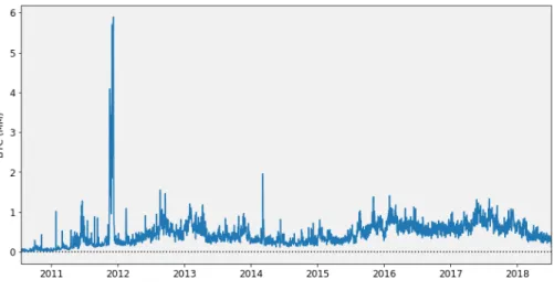
The time series of transaction fees (in percent of transaction volume) is depicted in Figure 3. The figure illustrates that, during most of the sample period, transaction fees charged by miners are low. Daily fees amount to .0109% of transaction volume, on average. Q1, median, and Q3 are .0038%, .0056% and .0104%, respectively. There are a few spikes, however. The largest one occurs towards the end of 2017, a time at which transaction fees exceeded 0.23%, due to the congestion triggered by the surge in trading volume (see Easley, O’Hara and Basu, 2018 or Huberman, Leshno and Moalleni, 2017 for models of blockchain transaction fees).
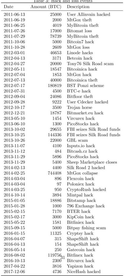
Browsing the web (in particular bitcointalk.org), we collected information about all hacks and other losses on bitcoin. We identified and collected data about 48 such events over our sampling period.10 We collected the amounts
8The Bitcoin protocol states that an output of a transaction (that is, an amount payed
to a particular bitcoin address), when spent, must be spent in full. Thus, if a bitcoin owner wants to transfer, e.g, 1 BTC to a payee, but owns 20 BTC as a single output of an earlier transaction, she has to create a transaction with one input (the 20 BTC) and two outputs: 1 BTC to an address belonging to the payee, and 19 BTC (abstracting from the fee payed to the miner of the block in which that transaction will be included) to herself. These 19 BTC are change money, and should not be counted as transaction volume.
9For that purpose, we eliminate outputs spent within less than 4 blocks, an heuristic
proposed by Kalodner et al. (2017).
10We have been unable to find information about the amount lost for the following three
events: the hack of the e-wallet service company Instawallet in April 2013; the hack of the South Korean exchange Bithumb reported in June 2017; the hack of the South Korean
ex-Figure 3: Transaction fees, in percent of estimated transaction volume
of the losses and the times at which they were reported. To obtain percentage losses (to fit our definition ofh), we divide lost amounts byXt. This time series is illustrated in Figure 4. The corresponding events are listed in Table 3. The largest loss is due to the collapse of Mt. Gox in February 2014, when 744,408 bitcoins were lost. On average, during the whole sample period, the fraction of bitcoins lost per week is approximately 0.04%.
We also collected information about events that are likely to affect the costs and benefits of using bitcoins. We distinguished between two types of events, relative to:
• The ease with which bitcoins can be bought or sold (MKT).
• The ease to use bitcoins to buy goods or services (COM).
For MKT, we identified 29 events over our sample period (see Table 4). Positive events include each time it became possible to exchange bitcoins against a new fiat currency (e.g., Euro or Yen) on a trading platform.11 Negative events include the shutdown of large platforms (such as Mt. Gox) or the ban of cryptocurrency trading platforms by China in September 2017.
For COM, we identified 30 events, which are listed in Table 5. Positive events include each time a new good or service can be purchased with bitcoins.
change Youbit in December 2017.
11We consider 11 fiat currencies for which bitcoin trading is significant: AUD, BRL, CAD,
CNY, EUR, GBP, JPY, KRW, PLN, RUR, TRY. USD in not in this list because trading against U.S. dollar began before the first day in our sample period. For each of these 11 fiat currencies, we select as the event date the first day for which trading data is available in at least one of the following two large-coverage, tick-by-tick datasets: Kaiko and bitcoincharts.com (seehttps://bitcoincharts.com/markets/list/). One exception is the Turkish Lira (TRY) for which no data is available. We find on the Web convincing information that trading on BTCTurk started on July 1, 2013, the day the exchange was first opened for trading.
Figure 4: Thefts and other losses of bitcoins, in percent of bitcoin supply
For example, on June 11, 2014, Expedia started accepting bitcoins for hotel reservations, while Microsoft accepted bitcoins from U.S. customers on Decem-ber 11, 2014. An example of negative news is when DELL no longer accepted bitcoins, on October 19, 2017. We consider both events concerning legal goods or services (e.g., hotel reservations, or desktop computers) and event concerning illegal goods and services (e.g., illegal drugs or firearms).
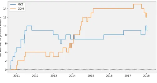
We classified each of these events as positive or negative news. We coded positive news as +1 and negative news as−1. We cumulated these positive or negative values to obtain indexes forMKT and COM. At each point in time, theMKT index quantifies how easy it is to buy or sell bitcoins, while theCOM index quantifies how easy it is to transform bitcoins into consumption goods and services. The time series of these indexes is illustrated in Figure 5.
TheMKTindex increases sharply during the first two years, as new exchange platforms allowing trades between bitcoins and new currencies open. TheCOM index remains low in the first years of the sample period, reflecting that it was hard to use bitcoins to purchase goods and services. It starts increasing towards the end of 2013 and reaches a relatively high level by 2015. The decrease towards the end of 2017 is due to a couple of large companies which stopped accepting payments in bitcoins.
5
Estimation and results
This section describes how we use the General Method of Moments (GMM) to estimate the equilibrium bitcoin pricing equation. It then presents estimation results followed by a robustness analysis based on ordinary least squares (OLS) estimation.
Figure 5: MKT and COM indexes
5.1
GMM estimation
We use GMM to estimate the non-linear equilibrium pricing equation in (18).12 We directly observe the fraction of bitcoins hackedhtand the bitcoin pricept. The transactional benefit of bitcoins (θt) is proxied by the COM index. For simplicity we assumeϕtis linear in Xt. Moreover, we assume the unit cost of trading bitcoin (ϕ0
t) can be proxied by two variables:
• The transaction fees in percent of (on-chain) volume, denotedBTC fee prcnt.
• An indexMKT invrs which is defined as 1/(1 +MKT), to make higher values correspond to higher costs and to make it asymptote to zero when takingMKT to infinity.
Therefore the model that is taken to the data requires the following “resid-ual” to be zero conditional on the timetinformation set:
et+1=Dt+1(1−ht+1) (1 +ρt+1)−1. (20) where the deflatorDt+1 is defined as
Dt+1=
1 +α0+α1∗COMt+1
1 +β0+β1∗BT C f ee prcntt+β2∗M KT invrst
. (21) We use standard GMM to estimate the parameters{α0, α1, β0, β1, β2}(for a detailed description see Appendix 6). The instrumental variables that are used in the estimation are all adapted to the information set at time t (i.e., their value is non-stochastic at that time). To reduce the risk of a weak instruments 12We refer to Cochrane (2005) for a thorough discussion of using GMM to identify in asset
problem, all variables correlate at least 5% with next period’s bitcoin return (i.e., the absolute value of the correlation is at least 0.05). This led to the following set of instrumental variables:
• An intercept term and year dummies for all years except for 2012 and 2017.
• All model variables evaluated at timet, including smoothed versions where at timetwe take an exponentially weighted value of historical observations with a half life equal to one month.
• Two additional variables that appear to correlate highly with future bit-coin return: the relative change in total bitbit-coin fees and the exponentially weighted value of the number of bitcoins hacked with a half-life of one year. The high correlation of these variables with next period’s bitcoin return is not surprising because extreme values for these variables are in-dicative of eventful times for the bitcoin investor. A full understanding of the exact channel that generates these correlations is beyond the scope of this paper. What is relevant is that there is correlation which, in equilib-rium, needs to be undone by picking the right bitcoin-return deflator Dt (i.e., by picking the true parameter values that generated the data).
Sample. To avoid day-of-the-week effects and keep a reasonable amount of data, the daily price series is downsampled to a weekly frequency. The fi-nal sample used in the estimation contains 388 observations and runs from the week of September 26, 2010, until the week of February 25, 2018.13 The average weekly bitcoin return expressed in USD in this period was 4.52%. The disper-sion in these returns was relatively high with a standard deviation of 17.9%, a minimum of -42.3%, and a maximum of 110%.
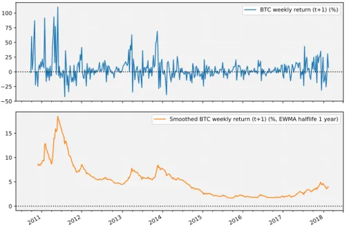
The top panel of Figure 6 plots the raw weekly bitcoin returns which we use in the estimation. The bottom panel plots smoothed returns which, by removing high frequency noise, helps visualise the low frequency trade. The figure suggests that required returns were positive throughout the sample. The larger trend seems to be a steady decline in the course of the sample, with a slight increase towards the end. We will revisit this pattern after model estimation. A decomposition of the (fitted) model-implied required return sheds light on what was driving this pattern (see Figure 7 and its discussion).
5.2
Results
As can be seen in Equation (20), it is difficult to identify separately the two constantsα0 and β0. To grasp the intuition consider the simple case in which
13Note that this weekly sample starts somewhat later and ends somewhat earlier than the
daily sample described in Section 4. The reason is that for the estimation we need a full sample and some data series used in the estimation either start late or finish early.
Figure 6: Bitcoin price data
This figure plots weekly Bitcoin returns expressed in USD. The top graph plots raw returns. The bottom graph smooths these returns with by plotting an exponentially weighted moving average of these returns with a half life of one year.
50 25 0 25 50 75 100 BTC weekly return (t+1) (%) 2011 2012 2013 2014 2015 2016 2017 2018 0 5 10 15
the benefits and costs of holding bitcoins are constant through time, i.e.,α1 =
β1=β2= 0. In that case, (20) simplifies to (when using (21))
et+1= (1−ht+1) 1 +α0 1 +β0
(1 +ρt+1)−1. Obviously, for each possible value of1+α0
1+β0, there is an infinite number of possible values of (α0, β0). So it is impossible to identifyα0andβ0. Whenα1,β1andβ2 are not set to 0, it is not strictly the case that α0 and β0 are not identified.14 But, trying to estimate both of them generates numerical instability and large standard errors. To avoid these problems we setα0to 0 and, when interpreting the estimate forβ0, we will bear in mind that it reflects the intercepts of both the costs and the benefits of holding bitcoins. Precisely, ifβ0 is estimated to be
ˆ
β0(hats refer to estimated values), then this implies that the intercept terms are estimated to be at the line (α0, β0) ={(x,βˆ0+x)|x∈R}. In other words, if one
believes the cost isxhigher than what ˆβ0+ ˆβ1BTC fee prcnt+ ˆβ2MKT invrs implies, the benefit should also bexhigher than what is implied by ˆα0+ ˆα1COM. It turns out that the issue becomes mute in our application under a relatively mild interpretation of the estimates.
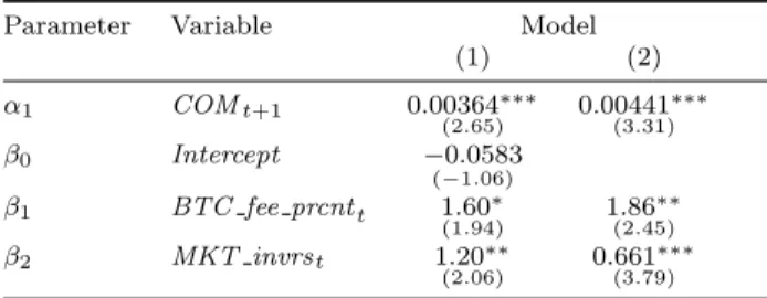
Table 1 presents the parameter estimates. Model (1) presents the param-eter estimates of the full model without any paramparam-eter constraint (other than
α0= 0). All parameters carry the predicted sign, but the intercept (β0) is not statistically significant and the coefficient for transactions fees is only marginally significant. The bitcoin required return, however, significantly decreases when there are more commercial opportunities ( ˆα1>0). And it significantly increases when the relative bitcoin fee is higher ( ˆβ1>0) or when bitcoin is easier to trade ( ˆβ2>0). To gauge the economic size of these effects we believe it is interesting to compute the model-implied bitcoin required return throughout our sample, and decompose into the components that drive it.
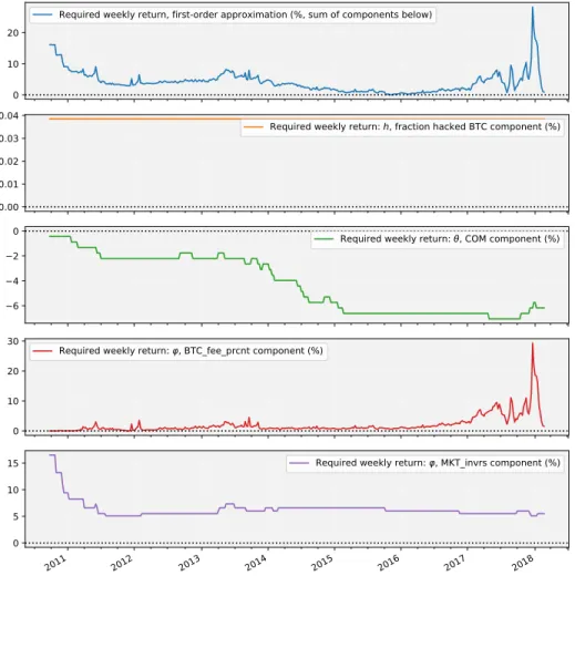
Before doing a required return decomposition we re-estimate the model with-out the insignificant intercept termβ0 to avoid reporting statistically insignifi-cant components. This yields the parameter estimation in model (2) of Table 1. All parameter retain their sign and become slightly more statistically significant. Figure 7 illustrates the economic size of each of the factors in the estimated bitcoin pricing equation of model (2) (see Table 1). The decomposition is based on the first-order expansion of the pricing equation presented in (19). We set Et[ht+1] to the sample average of ht and Et[θt+1] to θt+1. The latter assumes perfect foresight onθt+1 but setting Et[θt+1] =θt does not alter the decomposition asCOMt is a highly persistent series.
The figure leads to the following observations. First, the model-implied (weekly) required return on bitcoin hovers between 0% and 25%, with most values in the range of 5% to 10%. Second, the contribution of hack risk is small, as it amounts to 0.04%. Third, the transactional benefit starts out at 14Strictly speaking, the intercepts become mathematically identified, but only through
second-order terms. The first-order approximation of the model as derived in (19) shows that they are not identified in a first-order approximation.
Figure 7: Bitcoin required return
This figure plots the required Bitcoin return for the oncoming week along with its components based on a first-order approximation of the equilibrium pricing model. The top plot graphs the total required return and the four graphs below it decompose it into four components. The decomposition is based on model (2) in Table 1.
0 10 20
Required weekly return, first-order approximation (%, sum of components below)
0.00 0.01 0.02 0.03 0.04
Required weekly return: h, fraction hacked BTC component (%)
6 4 2
0 Required weekly return: , COM component (%)
0 10 20
30 Required weekly return: , BTC_fee_prcnt component (%)
2011 2012 2013 2014 2015 2016 2017 2018
0 5 10
Table 1: GMM estimates of model parameters
This table presents the GMM estimates of the model parameters.t-values are in parentheses and statistical significance is indicated by one, two, or three stars that correspond to a 10%, 5%, or 1% level, respectively.
Parameter Variable Model
(1) (2) α1 COMt+1 0.00364∗∗∗ (2.65) 0.00441 ∗∗∗ (3.31) β0 Intercept −0.0583 (−1.06) β1 BTC fee prcntt 1.60∗ (1.94) 1.86 ∗∗ (2.45) β2 MKT invrst 1.20∗∗ (2.06) 0.661 ∗∗∗ (3.79)
less than 1% but steadily rises to around 6%. This demonstrates that, with the commercial opportunities growing through time, the required return on bitcoin became substantially lower (i.e., 6% per week). Fourth, the relative fees for acquiring bitcoins did not command substantially higher returns on the bitcoin in equilibrium throughout the sample, with the exception of the final two years where it grew to 5% to 30% per week. Finally, the difficulty to convert bitcoins to cash added 15% to the required return on bitcoins initially, but within a year dropped to five percent weekly and stayed at this level throughout. Overall, the decomposition illustrates that the required return on bitcoin is economically significant and exhibits a non-trivial decomposition through time.
Finally, how much of the time variation in bitcoin returns can one attribute to a changing model-implied required return? Let us compute an R2. The standard deviation of the model-implied bitcoin required returns is 3.43%. For realized returns it is 17.9%. Time variation in required returns therefore only explains a small amount of time variation in realized returns. TheR2is 0.03432/0.1792= 3.67%. In other words, a large part of bitcoin returns seems driven by the multiplicative noise with mean one (see discussion on p. 11).
Robustness. Table 2 presents OLS estimates of the model parameters based on a linearized version of the model. Panel (a) presents these estimates and Panel (b) redoes estimation withall explanatory variables lagged so that the model becomes entirely predictive (and is therefore less exposed to endogeneity concerns). Note that the results echo the GMM results in terms of the signs of parameter coefficients and statistical significance, with the exception of the relative bitcoin fee. The fee is insignificant (but does have the correct sign in the multivariate models). The results therefore by and large testify to the robustness of the GMM results.
Table 2: OLS estimates of the linearized Bitcoin pricing model
This table presents the parameter estimates of the linearized model. The dependent variable is net Bitcoin return (i.e., net of fraction of hacked coins). t-values in parentheses. Panel (a) presents the results of OLS estimation of the linearized version of the equilibrium pricing equation that is estimated by GMM in Table 1. Panel (b) replicates Panel (a) with the exception that all explanatory variables are lagged. t-values are in parentheses and statistical significance is indicated by one, two, or three stars that correspond to a 10%, 5%, or 1% level, respectively.
Variable Model
(1) (2) (3) (4) (5) (6)
Panel (a): OLS estimate linearized model Intercept 0.045∗∗∗ (4.93) 0.10 ∗∗∗ (5.21) 0.049 ∗∗∗ (4.42) −0(−1..05756) 0.012 (0.26) COM −0.0057∗∗∗ (−3.27) −0.0052∗∗∗ (−2.68) −0.0049∗∗∗ (−3.05) BTC fee prcnt(-1) −0.33 (−0.59) 0.57 (0.95) (00..5898) MKT invrs(-1) 1.1∗∗∗ (2.88) 0.81 ∗∗ (2.09) 0.90 ∗∗∗ (5.65)
Panel (b): OLS estimate linearized model, all variables lagged Intercept 0.045∗∗∗ (4.93) 0.10 ∗∗∗ (5.20) 0.049 ∗∗∗ (4.42) −0.057 (−1.56) 0.011 (0.24) COM(-1) −0.0057∗∗∗ (−3.25) −0.0052∗∗∗ (−2.66) −0.0049∗∗∗ (−3.03) BTC fee prcnt(-1) −0.33 (−0.59) 0.57 (0.95) (00..5898) MKT invrs(-1) 1.1∗∗∗ (2.88) 0.81 ∗∗ (2.09) 0.90 ∗∗∗ (5.64)
6
Conclusion
We build an overlapping generations rational expectation equilibrium model relating the value of a cryptocurrency to the transactional costs and benefits it provides. The model shows that these fundamentals should be priced, and that their impact is magnified by expectations about future prices. The model implies that large volatility in bitcoin prices can be driven by extrinsically noisy changes in beliefs, and yet remains consistent with rational expectations about fundamentals.
We then confront the equilibrium pricing equation to a hand-collected dataset of fundamental events that affect the ease for agents to transact in bitcoins. We show that these fundamentals are significant determinants of bitcoin returns, and we provide quantitative measures of their relative importance over time. We also find that a large part of the variation in prices is unrelated to funda-mentals, and reflects extrinsic noise.
Appendix
Proof of Proposition 1
In the main text, we solved for prices and quantities under the assumption that consumption was strictly positive (i.e. the constraint cyt ≥ 0 did not bind). We show here that equation (6) also holds when considering explicitly the non-negativity constraint on young investors’ consumption.
Formally, letλbe the Lagrange multiplier associated with the constraint that young investors’ consumption be non-negative, cyt ≥0. With that constraint, the young investors’ optimization problem becomes
max qt,st,qˆt
u(cyt) +βEtu(cot+1) +λc y t
First-order conditions with respect toqt,stand ˆqtwrite, respectively −u0(cyt)pt+βEt u0(cot+1)(1−ht+1) (1 +θt+1) 1 +ϕ0(q t) pt+1 =λpt (22) −u0(cyt) +β(1 +rt)Et u0(cot+1) =λ (23) −u0(cyt)ˆpt+βEt u0(cot+1)ˆpt+1 =λpˆt (24)
Suppose λ > 0, i.e., the consumption non-negativity constraint binds. Then combining (22) and (23) yields the cryptocurrency pricing equation (6) in Propo-sition 1, which simplifies to (12) when investors are risk-neutral.
Similarly, combining (23) and (24) yields the central bank currency pricing equation: ˆ pt= 1 1 +rtE t u0(co t+1) Et[u0(cot+1)] ˆ pt+1
which simplifies to (15) when agents are risk-neutral. All the other derivations in the main text follow from these results.
Proof of Proposition 3:
¯ pt = λ t Y τ=1 uτ ! pt = λ t Y τ=1 uτ ! Et " K Y k=1 (1−ht+k) (1 +Tt+k) 1 +rt+k−1 ! pt+K # = λ t Y τ=1 uτ ! Et " K Y k=1 (1−ht+k) (1 +Tt+k) 1 +rt+k−1 ! t+K Y τ=t+1 ˜ uτ ! pt+K # = Et " K Y k=1 (1−ht+k) (1 +Tt+k) 1 +rt+k−1 ! λ t Y τ=1 uτ ! t+K Y τ=t+1 ˜ uτ ! pt+K # = Et " K Y k=1 (1−ht+k) (1 +Tt+k) 1 +rt+k−1 ! ¯ pt+K # ,which shows that each price ¯pt verifies (13). {p¯t} is therefore an equilibrium price sequence as long as ¯pt≤
eyt Xt+ϕt(Xt). QED
Details of the GMM estimation
We use standard two-step GMM to estimate the model. The GMM penalty function that was minimized with respect to the model parameters is:
P =m0W m∈R, (25)
where m is a vector that collects the inner products of the model’s residuals (e ∈ RT−1) and the n instrumental variables that appear as columns in V ∈ R(T−1)×n, and W ∈Rn×n is the standard weighting matrix. Formally, m can
be written as:15 m=V0e∈Rn×1 (26) where ( e= e2 · · · et+1 · · · eT 0 , v= v1 · · · vt · · · vT−1 0 ∈R(T−1)×1. (27) In the first step of the estimation the weighting matrixW is taken to be the identity matrix. The parameters estimated by minimizingP in this first step are then used to compute the moment covariance matrix which serves asW in the second step. The parameter estimates resulting from this second step are the final estimates.
15Note that the length of the time series isT −1 as opposed toT as next week’s residual
Statistical inference follows standard procedure. LetG∈Rn×n be the
gra-dient of then moments (i.e., the n elements ofm) used in the GMM penalty function in (25), with respect to the deep parameters. The covariance matrix of the estimators is:
G0 1 TM 0M −1 G !−1 , (28)
where M ∈ R(T−1)×n stacks the columns associated with the empirical
mo-ments. The first column, for example, is:
e◦v1∈R(T−1)×1, (29)
where ◦ is the Hadamard product (i.e., element-wise multiplication) and v1 is the first column ofV.
Numerical issues. To avoid landing in a local minimum, the numerical op-timization follows the following steps.
1. The penalty functionP in (25) is obtained by a brute-force minimization over an equal distance grid of candidate parameter values. The location of these grid points is informed by the OLS estimates of the model’s linearized version (see Section 5.2) in the following way. If X is the OLS estimate of a particular parameter, then the candidate values for this parameter are the 11 equidistant values in the interval [−|X|,|X|]. We center around zero to avoid stacking the deck in favor of finding the same parameter sign as in the OLS. We further inspect the grid point that minimizesP across the grid to ensure that we do not land at the edge of the grid (as this indicates the global minimum might be outside of the grid).
2. We fine-tune the grid-point estimate by starting a steepest-descent algo-rithm from this point. We further verify that the value algoalgo-rithm lands on a value, sayY, close to the grid point from where it departed. Close in this case means that the distance is smaller than the distance from the optimal grid point to any other point on the grid. If this is true, the procedure delivers theY as the final parameter estimate.
References
Athey, S., I. Parashkevov, V. Sarukkai and J. Xia, 2016, “Bitcoin Pricing, Adop-tion, and Usage: Theory and Evidence”, Stanford University Graduate School of Business Research Paper No. 16-42.
Auer, R., and S. Claessens, 2018, “Regulating cryptocurrencies: assessing mar-ket reactions”,BIS Quarterly Review, pp. 51-65.
Bianchi, D., 2017, “Cryptocurrencies as an asset class: an empirical assessment”, Working paper, Warwick Business School.
Borri, N. and K. Shakhnov, 2018, “Cryptomarket Discounts”, Working paper. Buraschi, A. and E. Pagnotta, 2018, “An Equilibrium Valuation of Bitcoin and
Decentralized Network Assets,”Working paper.
Chiu, J. and T. Koeppl, 2017, “The economics of cryptocurrencies - Bitcoin and beyond.”, Working paper, Queen’s University.
Cochrane, John H., 2005, “Asset Pricing ”, Revised Edition, Princeton Univer-sity Press.
Cong, L. W., Y. Li, and N. Wang., 2018, “Tokenomics: Dynamic Adoption and Valuation ”, Columbia Business School Working Paper.
Corbet, S., B. Lucey and L. Yarovaya, 2017, “Datestamping the Bitcoin and Ethereum bubbles”, Working paper, Dublin City University Business School. Easley, D., M. O’Hara, and S. Basu, 2018, “From Mining to Markets: The Evolution of Bitcoin Transaction Fees”, Working paper. Available at SSRN: https://ssrn.com/abstract=3055380 or http://dx.doi.org/10. 2139/ssrn.3055380.
Fantazzini, D., E. Nigmatullin, V. Sukhanovskaya, and S. Ivliev, 2016, “Every-thing you always wanted to know about bitcoin modelling but were afraid to ask: Part 1”,Applied Econometrics 44, pp. 5-24.
Fern´andez-Villaverde, J., and D. Sanchez, 2018, “On the Economics of Digital Currencies”, Federal Reserve Bank of Philadelphia Working Paper.
Gaballo, G. and E. Mengus, 2018, “Time-Consistent Fiscal Guarantee for Mon-etary Stability”, Working paper, HEC Paris.
Garratt, R. and N. Wallace, 2018, “Bitcoin 1, Bitcoin 2...: an experiment with privately issued outside monies”,Economic Inquiry, 56 (3), pp. 1887-1897. Hendry, S. and Y. Zhu, 2018, “A Framework for Analyzing Monetary Policy in
Huberman, G., J. Leshno, and C. Moalleni, 2017, “Monopoly without a monop-olist: an economic analysis of the bitcoin payment system”,CEPR discussion paper 12322.
Kalodner, H., S. Goldfeder, A. Chator, M. M¨oser, and A. Narayanan, “BlockSci: Design and applications of a blockchain analysis platform”, Working paper, 2017. arXiv:1709.02489v1
Kareken, J. and N. Wallace, 1981, “On the Indeterminacy of Equilibrium Ex-change Rates”,Quarterly Journal of Economics 96(2), pp. 207-222.
Lagos, L. and R. Wright, 2005, “A unified framework for monetary theory and policy analysis ”,Journal of Political Economy, pp. 463-484.
Liu, Y. and A. Tsyvinski, 2018, “Risks and returns of cryptocurrency.” Working paper, Yale University.
Makarov, I., and A. Schoar, 2018, “Trading and Arbitrage in Cryptocur-rency Markets”, Working paper. Available at SSRN: https://ssrn.com/ abstract=3171204orhttp://dx.doi.org/10.2139/ssrn.3171204. Meiklejohn S., M. Pomarole, G. Jordan, K. Levchenko, D. McCoy, G. M.
Voelker, and S. Savage, “A fistful of bitcoins: characterizing payments among men with no names”, In Proceedings of the 2013 conference on Internet mea-surement conference (IMC ’13). ACM, New York, NY, USA, pp. 127-140.
DOI:https://doi.org/10.1145/2504730.2504747
Obstfeld, M. and K. Rogoff, 1983, “Speculative Hyperinflations in Maximizing Models: Can We Rule Them Out”, Journal of Political Economy 91, pp. 675–687.
Pagnotta, E., 2018, “Bitcoin as Decentralized Money: Prices, Mining Rewards, and Network Security,” Working Paper.
Prat, J., and B. Walter, 2018, “An Equilibrium Model of the Market for Bitcoin Mining,” Working Paper.
Saleh, F., 2018, “Volatility and Welfare in a Crypto Economy,” Working Paper. , Samuelson, P., 1958, “An Exact Consumption-Loan Model of Interest with or without the Social Contrivance of Money,” Journal of Political Economy 6, pp 467-482.
Schilling, L. and H. Uhlig, 2018, “Some Simple Bitcoin Economics,” NBER Working Paper No. 24483.
Shiller, R, 1981, “Do Stock Prices Move Too Much to be Justified by Subsequent Changes in Dividends?” American Economic Review 71, pp 421-36.
Tirole, J., 1985, “Asset bubbles and overlapping generations,” Econometrica, pp 1499-1528.
Wallace, N., 1980, “The Overlapping Generations Model of Fiat Money” in Neil Wallace and John H. Kareken, eds., Models of Monetary Economics, Minneapolis, MN, Federal Reserve Bank of Minneapolis.
Zimmerman, P, 2018, “Blockchain and price volatility” mimeo Said Business School.
Table 3: Hack and loss events Date Amount (BTC) Description
2011-06-13 25000 User Allinvain hacked 2011-06-19 2000 MtGox theft 2011-06-25 4019 MyBitcoin theft 2011-07-26 17000 Bitomat loss 2011-07-29 78739 MyBitcoin theft 2011-10-06 5000 Bitcoin7 hack 2011-10-28 2609 MtGox loss 2012-03-01 46653 Linode hacks 2012-04-13 3171 Betcoin hack
2012-04-27 20000 Tony76 Silk Road scam 2012-05-11 18547 Bitcoinica hack 2012-07-04 1853 MtGox hack 2012-07-13 40000 Bitcoinica theft 2012-07-17 180819 BST Ponzi scheme 2012-07-31 4500 BTC-e hack 2012-09-04 24086 Bitfloor theft 2012-09-28 9222 User Cdecker hacked 2012-10-17 3500 Trojan horse
2012-12-21 18787 Bitmarket.eu hack 2013-05-10 1454 Vircurex hack 2013-06-10 1300 PicoStocks hack
2013-10-02 29655 FBI seizes Silk Road funds 2013-10-25 144336 FBI seizes Silk Road funds 2013-10-26 22000 GBL scam
2013-11-07 4100 Inputs.io hack 2013-11-12 484 Bitcash.cz hack 2013-11-29 5896 PicoStocks hack
2013-11-29 5400 Sheep Marketplace closes 2014-02-13 4400 Silk Road 2 hacked 2014-02-25 744408 MtGox collapse 2014-03-04 896 Flexcoin hack 2014-03-04 97 Poloniex hack 2014-03-25 950 CryptoRush hacked 2014-10-14 3894 Mintpal hack 2015-01-05 18886 Bitstamp hack 2015-01-28 1000 796 Exchange hack 2015-02-15 7170 BTER hack 2015-02-17 3000 KipCoin hack 2015-05-22 1581 Bitfiniex hack 2015-09-15 5000 Bitpay fishing scam 2016-01-15 11325 Cryptsy hack 2016-04-07 315 ShapeShift hack 2016-04-13 154 ShapeShift hack 2016-05-14 250 Gatecoin hack 2016-08-02 119756 Bitfinex hack 2016-10-13 2300 Bitcurex hack 2017-04-22 3816 Yapizon hack 31
Table 4: MKT events Date Effect Description
2010-09-14 1 BTCex RUR/BTC exchange opens 2010-10-25 1 MtGox eases fund transfers
2010-12-01 1 BTCex JPY/BTC exchange opens
2010-12-07 1 MtGox partners with e-payment company Paxum 2011-01-04 1 Bitcoin-Central EUR/BTC exchange opens 2011-03-30 1 GBP/BTC exchange opens
2011-04-01 1 Bitomat PLN/BTC exchange opens
2011-06-04 -1 The Bitcoin Market discontinues PayPal trading 2011-06-08 1 CaVirTex CAD/BTC exchange opens
2011-06-13 1 BTCC China CNY/BTC exchange opens 2011-06-18 1 Bitmarket.eu AUD/BTC exchange opens 2011-07-28 1 Mercado Bitcoin BRL/BTC exchange opens 2012-02-10 -1 Paxum exits bitcoin business
2013-04-03 -1 MtGox experiences outages
2013-04-10 -1 MtGox and other exchanges experience outages 2013-05-14 -1 MtGox suspends fund transfers
2013-07-01 1 BTCTurk BTC/TRY exchange opens 2013-09-03 1 Korbit BTC/KRW market opens 2013-12-18 -1 BTC China suspends deposits in yuan 2014-01-30 1 BTC China reinstates deposits in yuan 2014-02-25 -1 MtGox shuts down
2015-10-08 1 Gemini offers FDIC-insured dollars deposits 2016-11-14 1 CME launches bitcoin reference rate 2017-09-30 -1 Chinas exchanges shutdown
2017-12-10 1 Future trading starts at CBOE 2017-12-17 1 Future trading starts at CME
Table 5: COM events Date Effect Illegal Description 2011-01-23 1 1 Silk Road opens 2011-02-25 1 0 CoinCard service opens 2011-06-08 1 0 BTC Buy service opens 2011-06-30 1 1 Black Market Reloaded opens
2012-09-04 -1 0 CoinCard trading service permanently closed 2012-11-15 1 0 WordPress accepts bitcoin
2013-04-03 -1 0 BTC Buy stops selling prepaid cards 2013-05-09 1 0 Gyft accepts bitcoin
2013-08-27 1 0 eGifter accepts bitcoin 2013-10-02 -1 1 Silk Road closes 2013-11-06 1 1 Silk Road 2.0 opens
2013-11-22 1 0 CheapAir accepts bitcoin for flights 2013-12-02 -1 1 Black Market Reloaded closes 2014-01-09 1 0 Overstock.com accepts bitcoin 2014-01-24 1 0 TigerDirect accepts bitcoin
2014-02-03 1 0 CheapAir accepts bitcoin for hotel reservations 2014-06-11 1 0 Expedia accepts bitcoin for hotel reservation 2014-07-01 1 0 Newegg accepts bitcoin
2014-07-18 1 0 Dell accepts bitcoin
2014-08-14 1 0 DISH Network accepts bitcoin 2014-11-06 -1 1 Silk Road 2.0 closes
2014-12-11 1 0 Microsoft accepts bitcoin from US customers 2015-01-22 1 0 Paypal accepts bitcoin
2015-02-19 1 0 Dell Expands bitcoin payments to UK and Canada 2017-04-27 1 0 Valve accepts bitcoin
2017-10-19 -1 0 Dell no longer accepts bitcoin 2017-12-06 -1 0 Steam no longer accepts bitcoin 2017-12-26 -1 0 Microsoft no longer accepts bitcoin 2018-01-09 1 0 Microsoft resumes bitcoin payments