GUIDO PEZZINI
Abstract. These notes are an introduction to wonderful varieties. We discuss some general results on their geometry, their role in the theory of spherical varieties, several aspects of the combinatorics arising from these varieties, and some examples.
1. Introduction
These notes are based on a series of lectures given by Michel Brion and Ja-copo Gandini on wonderful varieties, in occasion of the “Workshop on Spherical Varieties”, held from October 31 to November 4, 2016 at the Tsinghua Sanya In-ternational Mathematics Forum.
Wonderful varieties first appeared in the work of De Concini and Procesi, as compactifications (with remarkable properties) of symmetric spaces G/Gθ, where
Gis a semisimple linear algebraic group andθ:G→Gis an involution (see [DP83]). One of their motivations was to attack problems in classical enumerative geometry. These varieties include several ones studied in the theory of reductive groups, such as the variety of complete conics, or the space of complete collineations. Among the most important cases we may also mention the wonderful compactifications of adjoint semisimple groups, which have many relevant applications.
Later, Luna considered more general varieties, defining them wonderful if they have the same main properties of the De Concini-Procesi compactifications (see Def-inition 2.5). Such varieties have been then better understood, and have a central role, in the theory ofspherical varieties. Knop proved in [Kn96] that, in a precise sense, there are “enough” wonderful varieties among the spherical ones (see The-orem 4.3 below). This enabled Luna to initiate in [Lu01] a classification program for spherical varieties, built around studying the wonderful case. This program has been completed recently, see [BP16] and references therein.
Acknowledgements
Many thanks are due to Baohua Fu and Michel Brion for organizing the workshop at the Tsinghua Sanya International Mathematics Forum. I also thank Michel Brion, Baohua Fu and Jacopo Gandini for useful exchanges on the topics of the lectures, and a referee for useful remarks and suggestions.
2. Definitions and examples
Throughout the paper, the ground field will be the field of complex numbersC. We fix a connected reductive groupG, and, unless otherwise stated, we fix a Borel subgroupB ⊆G, a maximal torusT ⊆B, we denote bySthe corresponding set of
Date: April 27, 2017.
simple roots, andW the Weyl group. Given an algebraic groupH, we denote by X(H) its group of characters, by Hr its radical, byHu its unipotent radical, and
byZ(H) its center.
Wonderful varieties areG-varieties where the orbit structure is particularly nice. Their structure is similar to the following basic example.
Example 2.1. Letn≥1 andG= (C∗)n, which acts on Cn by multiplication
(t1, . . . , tn)·(x1, . . . , xn) = (t1x1, . . . , tnxn).
TheG-stable prime divisors, i.e. the coordinate hyperplanes, are smooth and
inter-sect transversally. The interinter-section of any subset of such divisors is non-empty and is an orbit closure, and all orbit closures are obtained in this way.
It is easy to give examples where the orbit structure does not fulfill these prop-erties.
Example 2.2. The group SL(n) acting linearly on Cn (with n ≥ 2) has two
orbits, namely{0} and its complement. The orbit{0}, which is closed, is not the intersection ofG-stable prime divisors.
Our goal is to give a general definition forcompleteG-varieties, where the orbit structure resembles the one in Example 2.1. We start with the following.
Definition 2.3. LetX be a smooth variety, andD1, . . . , Dr⊂X prime divisors.
The divisorD=D1+. . .+Drhasstrict normal crossingsif, for allp∈X, anyDi
containingphas a local equation inOX,p, and the set of these local equations can
be completed to a local system of parameters ofOX,p.
If a divisor D =D1+. . .+Dr as above has strict normal crossings, then the
componentsD1, . . . , Dr are smooth. They induce a stratification ofX into locally
closed smooth subvarieties, indexed by subsetsI⊆ {1, . . . , r}, namely the varieties
XI = \ i∈I Di ! r [ j /∈I Dj .
Notice that we do not require yet that the intersectionD1∩. . .∩Dris non-empty.
Example 2.4. Letn ≥2 and X =P(Cn⊕C) with its natural action of SL(n),
and define Y = Blp(X) where p= [0, . . . ,0,1]. Then the action of SL(n) lifts to
an action onY, andY has exactly two SL(n)-stable prime divisors. Their sum has strict normal crossings, but their intersection is empty.
We come to our main definition.
Definition 2.5 (Luna). Let X be an irreducibleG-variety. ThenX is wonderful (of rank r) if it is smooth, complete, it has exactly r prime divisors D1, . . . , Dr
that are G-stable, and in addition they have strict normal crossings, non-empty intersection, and the stratumXI is aG-orbit for allI⊆ {1, . . . , r}.
Remark 2.6. LetX be a wonderfulG-variety of rankr.
(1) The variety X has 2r G-orbits; among them, exactly one is open, namely X∅, and exactly one is closed, namely X{1,...,r}.
(2) SinceX is in particular normal with only one closedG-orbit, it follows by [Su74] thatXis projective, and a standard argument yields that the radical ofGacts trivially onX.
Wonderful varieties play a crucial role in the theory of spherical varieties, let us recall the definition.
Definition 2.7. An irreducible normalG-varietyX issphericalif a Borel subgroup ofGhas an open orbit onX.
A spherical variety has in particular an openG-orbit; the stabilizerH of a point on this G-orbit (so that the latter is the homogeneous space G/H) is called a spherical subgroupofG.
The first observation we make to relate the two definitions above is the following. Theorem 2.8 ([Lu96]). Any wonderful variety is spherical.
We point out that all requirements of Definition 2.5 are necessary to have spheric-ity, as seen in the next example.
Example 2.9 ([Lu96]). Consider X =P(C2)×P(Sym2(C2)) under the action of
G = SL(2). Then X is smooth and projective, it has exactly 4 orbits and two smoothG-stable prime divisors which intersect in a singleG-orbit. More precisely,
one G-stable prime divisor is P(C2)×Y, where Y is the unique G-stable prime
divisor of P(Sym2(C2)). We recall that any point ofP(Sym2(C2)) can be written
as a product [v·w] for somev, w∈C2r{0}, and thatY is the set of the points of
the form [v·v] wherev∈C2r{0}. The other G-stable prime divisor of X is the
set of points ([u],[v·w]) withu, v, w∈C2r{0} such thatCu=Cv or Cu=Cw.
It is elementary to write local equations of these divisors, and conclude that they have the same tangent space in any point of their intersection, which is a single
G-orbit. As a consequence, they don’t have strict normal crossings, andX is not
spherical since it has dimension 3. It is also possible to construct SL(2)-varieties of dimension 3, where all G-stable prime divisors have strict normal crossings but empty intersection (see [MJ88]).
Let us give some examples of wonderful varieties.
Example 2.10. (1) An irreducible G-varietyX is wonderful of rank 0 if and only if it is homogeneous and complete. This is equivalent to being a partial flag varietyX=G/P, whereP is a parabolic subgroup ofG.
(2) An irreducible complete normalG-variety X is wonderful of rank 1 if and only if it has two G-orbits, one open and one of codimension 1. Such varieties are classified, see [Ah83] and [Br88]. Let us give some examples.
(a) The product X =P1×P1, with diagonal action of G= SL(2). The
G-stable prime divisor is the diagonal.
(b) The varietyX=P2=P(Sym2(C2)) under the action ofG= SL(2).
(c) The variety X = P(M2), where M2 is the vector space of (2× 2)-matrices, under the action ofG= GL(2)×GL(2) induced by left and right multiplication. The points corresponding to matrices of rank 1 form theG-stable prime divisor.
(3) Wonderful varieties of rank 2 have been classified in [Wa96]. A classical example is the variety ofcomplete conics, which is the variety
X={([A],[B])∈P(M3)×P(M3)|AB∈C·13×3}.
where we denote by Mn the space of (n×n)-matrices, and by 1n×n the
unit matrix. The varietyX is the wonderful compactification of the homo-geneous space SL(3)/SO(3)Z(SL(3)), which is the space of smooth conics
inP2. The twoG-stable prime divisors ofX are:
D1 = {Anon-invertible}, D2 = {B non-invertible}.
(4) Let us describe an example of rank 3 (see [Pe09, Section 3.5]). Let G= Sp(2a)×Sp(2b) (with a, b ≥2), and call Ω, Ω0 the bilinear forms on C2a
and C2b defining Sp(2a) and Sp(2b). For k, n ∈ N, denote by Grk(Cn)
the Graßmannian of k-dimensional vector subspaces of Cn. Consider the
variety X= (E, F, p) E∈Gr2(C2a), F ∈Gr2(C2b), p∈P(Hom(E, F)) ,
where Gacts in a natural way. Under this actionX is wonderful of rank 3, withG-stable prime divisors:
D1 = {rankM = 1}, D2 = {Ω|E1= 0}, D3 = {Ω0|E2 = 0}. where we setp= [M] forM ∈Hom(E, F).
(5) An example of higher rank is given by the space ofcomplete collineations (see [Se51]). It is a wonderful variety of rankrforG= GL(r+1)×GL(r+1), where r≥1. We can describe it starting from the variety Y =P(Mr+1), which is a G-variety under left and right multiplication. Notice that Y has r+ 1 orbits, whose closures Zr+1 ⊃Zr ⊃ . . . ⊃Z1 are given by the condition thatZi is the set of points corresponding to matrices of rank at
most i. While Y is not a wonderful variety (if r ≥ 2), we can blow up
Y successively along the (strict transform of) Z1, . . . , Zr−1, and obtain a
wonderful varietyX. Its open G-orbit is isomorphic to PGL(r+ 1), hence X is a wonderful compactification of this group.
We end this section with an easy observation on the geometry of wonderful varieties.
Proposition 2.11. Let X be a wonderful variety of rank r as in Definition 2.5, andI⊆ {1, . . . , r}. Then
XI =XI =
\
i∈I
Di
is a wonderful variety, of rankr− |I|.
3. The local structure theorem
We discuss in this section the fundamental result of Brion, Luna, and Vust on the local structure ofG-varieties, applied to the wonderful case.
Let X be a wonderfulG-variety of rank r. Its closed G-orbit Y is a complete homogeneous space forG, so it is isomorphic to a quotient of the formG/Q, where Qis the stabilizer of a pointy∈Y, and it is a parabolic subgroup ofG.
Denote byP a parabolic subgroup ofGopposite toQ, i.e. such thatP∩Q=L is a Levi subgroup ofP andQ. Denote byPu the unipotent radical ofP.
Theorem 3.1([BLV86]). Under the above assumptions, there exists a locally closed affine subvariety Z ⊆X containing y such that Z is L-stable, and such that the map
Pu×Z → X
(g, x) 7→ gx
is an open P-equivariant immersion, where an element p∈P acts onPu×Z as vl·(u, z) = (vlul−1, lz), whereu, v∈Pu,l∈L,z∈Z, andp=vl.
The above theorem holds in this form for varieties that are much more general than wonderful ones. However, since X here is wonderful, the structure of the varietyZ is very particular, and motivates further the analogy with Example 2.1. Proposition 3.2. A varietyZ as in Theorem 3.1 is isomorphic to the affine space
Ar, on whichLacts asg·(u1, . . . , ur) = (σ1(g)u1, . . . , σr(g)ur)whereσ1, . . . , σrare
linearly independent characters of L. Moreover, under the isomorphism Z ∼=Ar,
the intersectionDi∩Z is identified with{ui= 0} for alli∈ {1, . . . , r}.
Proof. Consider the pointy∈Z∩Y as above. Recall that the orbit mapPu→Y
sending g to gy is an open immersion by the Bruhat decomposition of Y. Then Theorem 3.1 impliesZ∩Y ={y}, and also thatZ is smooth of dimensionr.
SinceX is wonderful, there exist local coordinatest1, . . . , tr aroundy such that
ti is a local equation of Di for all i. Theorem 3.1 implies the restrictionvi=ti|Z
is a local equation ofDi∩Z inZ in a neighborhood of the pointy.
We may suppose thatvi ∈C[Z]. Then the classesv1, . . . , vrare a basis ofmy/m2y,
where we denote bymy the maximal ideal inC[Z] of the pointy.
The ideal my is a rational L-module, and m2y is a submodule. Since Di∩Z is
L-stable for all i, the classvi is an L-eigenvector. SinceLis reductive, we can lift
these classes toL-eigenvectorsu1, . . . , ur∈my. Notice that (L, L) fixesu1, . . . , ur,
therefore it acts trivially onZ.
TheL-eigenvectorsu1, . . . , ur ∈my have linearly independent weights, because
otherwise a monomial un1
1 · · ·unrr (with exponents not all zero) would be a
non-constant element ofC(Z)L. But the latter is equal to
C(X)P by Theorem 3.1, and
this field isCby Theorem 2.8. We also deduce thatLhas an open orbit onZ. At this point [Lu73, Corollaire 2, p. 98] implies thatZ= SpecC[u1, . . . , ur]∼=Ar.
Moreover, the subsets {u1 = 0}, . . . ,{ur = 0} ofZ are its uniqueL-stable prime
divisors, hence they coincide with resp.D1∩Z, . . . , Dr∩Z.
From now on, we fix a Borel subgroup B ⊆ G contained in P. We give some definitions for the wonderful varietyX, taken from the theory of spherical varieties. Definition 3.3. With the above notations, we define:
(1) the set ∆(X) of theB-stable, notG-stable prime divisors ofX, called the colorsofX,
(2) the set Σ(X) ={σ1, . . . , σr}, whose elements are called the spherical roots
ofX.
(3) the lattice Ξ(X) of theB-eigenvalues of B-eigenvectors ofC(X).
Remark 3.4. Thanks to Proposition 3.2, the spherical roots of X are also the weights ofT acting on the normal spaceTX,y/TY,y.
Example 3.5. It is not difficult to compute Σ(X) for X equal to the space of complete conics, using the definition we have given in Example 2.10: we have Σ(X) ={2α1,2α2}, whereα1, α2are the simple roots of SL(3).
Lemma 3.6. The setΣ(X)is a basis of Ξ(X).
Proof. LetC(X)(B)be the multiplicative group of rational functions onX that are
B-eigenvectors. By Theorem 3.1 we have C(X)(B) =
C(Z)(B∩L), and the lemma
follows from Proposition 3.2.
Proposition 3.7. The openB-orbit ofX is equal toPu·Z0, whereZ0is the open
L-orbit of Z. Moreover, we have
Xr(Pu·Z) = [
D∈∆(X) D.
Proof. The first assertion is clear thanks to Theorem 3.1 and Proposition 3.2, let us show the second one.
LetD∈∆(X). If Dintersects Pu·Z then the intersection is aB-stable prime
divisor of Pu·Z ∼= Pu×Z, so it is of the form Pu×E where E is a (B∩
L)-stable prime divisor ofZ. But then E is one of coordinate hyperplanes ofZ, and D∩(Pu·Z) coincides withD
i∩(Pu·Z) for somei. This yieldsD=Di, contradicting
the assumption thatD is notG-stable. SoD⊆Xr(Pu·Z).
Conversely, the setXr(Pu·Z) has pure codimension 1, sincePu·Z ∼=Pu×Zis
affine. LetD be one of its irreducible components: it isB-stable becausePu·Z is
B-stable, andDis notG-stable because it cannot contain the unique closedG-orbit
Y. HenceD∈∆(X), and the proof is complete. Proposition 3.8([Br89]). The Picard group ofX is freely generated by the classes of the colors, and the classes of theG-stable prime divisors are linearly independent. Proof. LetD be a divisor ofX, and let D0 be the linear combination with same coefficients only of the prime divisors of D that are not colors. Since X0 =Xr S
D∈∆(X)D is an affine space, the divisorD0 is principal inX0, i.e.D0= (f) for some f ∈C(X0). But thenD−(f), where the divisor (f) is taken now inX, is a
linear combination of colors.
In other words, up to linear equivalence we may assumeD0 = 0. If now D is principal inX, withD= (f) for somef ∈C(X), thenf|X0 is a nowhere-vanishing regular function onX0. It follows that f is constant, andD= 0.
This shows the first assertion of the proposition. To show the second, suppose that a linear combination a1D1+. . .+arDr is principal, so it is equal to (f) for
some f ∈C(X). Then f restricts to a nowhere-vanishing regular function on the
openG-orbitG/H ofX. Pull-backf along the quotientG→G/H. By [KKV89,
Proposition 1.2], this pull-back is a character ofGup to a multiplicative constant: since the radical of G acts trivially onX, we conclude that f is constant and so the coefficientsa1, . . . , ar are all 0.
Thanks to the above proposition, we can express for allithe class [Di] ofDi as
a linear combination of the classes of the colors, enabling us to give the following. Definition 3.9. We define theCartan pairingofX as the map
c: ∆(X)×Σ(X)→Z such that [Di] = X D∈∆(X) c(D, σi)[D]
Often the Cartan pairing is extended linearly to a map c: spanZ∆(X)×spanZΣ(X)→Z.
Remark 3.10. To compute the Cartan pairing in practice, we can use Proposi-tions 3.2 and 3.7. They imply that a G-stable prime divisor Di of a wonderful
variety X has a local equation fi ∈ C(X) around the point y, such that fi is a
B-eigenvector ofB-eigenvalue−σi. Moreover, thanks to the two propositions
men-tioned above, the order of fi along any otherG-stable prime divisor is 0, and any
other zero or pole offiis a color. It follows that the corresponding principal divisor
isDi−PD∈∆(X)c(D, σi)D. We may rephrase this analysis as follows: the Cartan
pairing c(D, σi), for D ∈ ∆(X) is equal to the valuation of fi−1 along the prime
divisorD.
Example 3.11. AssumeGis adjoint, and identify it with theG×G-homogeneous (symmetric) spaceX0 =G×G/diag(G). ThenX0 has a G×G-equivariant won-derful completionX thanks to the work of De Concini and Procesi. Let us denote byB− the Borel subgroup ofGopposite toB with respect toT; we fix the Borel
subgroupB×B− ofG×Gand the maximal torus T×T.
We have Ξ(X) = {(χ,−χ) | χ ∈ X(T)}. The spherical roots of X are the elements (α,−α), whereαis any simple root of G. We can also choose the Borel subgroupB×B ofG×Ginstead. With this choice, we consider the set of simple roots ofG×Gas the union of the sets of simple roots of the two factors G. For a simple root αof the first factor G, define α0 in such a way that−w0(α0) is the
simple root of the second factor G corresponding to α, where w0 is the longest element of the Weyl group ofG. Then the spherical roots ofX are the set
Σ(X) ={α+α0 |αsimple root ofG}.
Let us get back to the choice of the Borel subgroupB×B−⊆G×G. The colors
ofX are the closures of theB×B−-stable prime divisors ofX0, and these are the irreducible components ofX0rBB−, sinceBB− is the openB×B−-orbit ofX0. Let us compute the Cartan pairing c: ∆(X)×Σ(X) → Z. Denote by Ge the
universal cover of G, and byωα the fundamental dominant weight corresponding
to a simple root αofG. LetV(ωα) be the irreducibleG-module of highest weighte
ωα, choose a highest weight vector vα ∈V(ωα), and a lowest weight vector ηα in
the dual moduleV(ωα)∗. Recall thatηαhas weight−ωα.
With these assumptions the matrix coefficientFα:g 7→ hηα, g−1vαiis a global
equation inC[G] of a divisore DeαofG. We have thate Deαis the pull-back onGe of a
B×B−-stable prime divisorDα,0 ofX0, so the closureDα=Dα,0 inX is a color ofX. All colors ofX are obtained in this way.
Finally, the functionFα is (B×B−)-semiinvariant, of weight (ωα,−ωα), hence
the product
fα=
Y
βsimple root
Fβhα,β∨i
is a (B×B−)-semiinvariant rational function onX with (B×B−)-weight equal to
(α,−α). Thanks to Remark 3.10, we conclude thatc(Dα,(α,−α)) is equal to the
order offα alongDα, i.e. the Cartan pairingcofX is given by the Cartan matrix
4. The logarithmic tangent bundle
We begin this section recalling some basic facts on aG-varietyX, only assuming it is smooth and irreducible. For more details, we refer to [Br07, Section 2].
For a pointx∈X, consider the orbit mapG→Xsendinggtogx. Its differential in the neutral elemente∈Gis a linear map
θx:g→TX,x
where gis the Lie algebra of G andTX,x is the tangent space ofX in x. Notice
thatθx is surjective if and only if the orbitG·xis open inX.
This picture can be globalized: denote byTX the sheaf of sections of the tangent
bundle of X, and denote bygthe constant sheaf on X associated tog. Then the
G-action induces a morphisms of sheaves onX
θ:OX⊗g→ TX.
Notice that X is G-homogeneous if and only if this morphism of sheaves is surjective.
Let now D = D1 +. . .+Dr be a divisor on X with strict normal crossings
as in Definition 2.3. ConsideringTX as the sheaf of derivations Der(OX), we can
consider the subsheaf of derivations stabilizing the ideal sheafOX(−D) ofD, and
we denote it byTX(−D). It is locally free, and it is called thelogarithmic tangent
sheafof the pair (X, D).
Remark 4.1. Letn= dim(X), son≥r. Fixx∈X, and denote byI the subset of {1, . . . , r} such that x ∈ Di if and only if i ∈ I. Denote by t1, . . . , tn local
coordinated around x, such that ti = 0 is a local equation of Di for all i ∈ I.
Then TX(−D) is generated, locally around x, by ti∂t∂i for i ∈ I, and by
∂ ∂tj for
j∈ {1, . . . , n}rI.
IfGacts onX preservingD, thenθmapsOX⊗gtoTX(−D), and we have the
following.
Proposition 4.2. If X is wonderful then θ:OX ⊗g → TX(−D) is surjective.
Moreover, the kernel kerθx (contained in the stabilizer gx) is the kernel of the gx-action on the normal spaceTX,x/TGx,x.
Proof (sketch). The proof is reduced, thanks to Theorem 3.1 and Proposition 3.2,
to the elementary case of Example 2.1.
The above proposition implies that, for all pointsxof ann-dimensional wonderful varietyX, the kernel kerθxis a Lie subalgebra ofgof codimensionn. This induces
theDemazuremorphism
f: X → Grn(g)
x 7→ kerθx
where Grn(g) is the Graßmannian ofn-codimensional vector subspaces ofg. We end this section summarizing in the following theorem several important results on wonderful varieties.
Theorem 4.3. Let X be a wonderful variety, with openG-orbitG/H. (1) The quotientNG(H)/H is finite.
(2) IfH=NG(H)thenf:X→Grn(g)is an immersion. In particularNG(H)
is the stabilizer of the Lie algebra hofH under the adjoint action ofGon
(3) For any spherical subgroupK⊆Gsuch thatK=NG(K)the homogeneous
spaceG/K admits a wonderful completion.
Proof (references). The first assertion follows from [BrPa87, Corollaire 5.3]. The second is proved in [Lo09b]. The third assertion is a fundamental theorem of Knop,
see [Kn96].
5. Spherical roots and colors
The finite sets ∆(X) and Σ(X), which we attach to any wonderfulG-varietyX, have a quite rich combinatorial structure. It generalizes the combinatorial part of the theory of symmetric spaces.
The first main result we mention is Theorem 5.1 below. Before stating it, we recall that the spherical roots can be defined also for a general spherical variety. Correspondingly, Theorem 5.1 can be stated also for a general spherical variety; it is due to Brion in characteristic 0 (see [Br90]), and to Knop in odd characteristic (see [Kn14]).
LetX be a wonderfulG-variety. We equip Ξ(X)⊗ZQwith an inner product by
restricting aW-invariant inner product onX(T)⊗ZQ.
Theorem 5.1([Br90, Kn14]). LetX be a wonderful variety. The setΣ(X)is the set of simple roots of a root system.
We denote byW(X) the Weyl group of the root system generated by Σ(X). It is called thelittle Weyl groupofX, and generalizes the little Weyl group classically defined for symmetric spaces.
Also the set of colors ∆(X), equipped with the Cartan pairingc: ∆(X)×Σ(X)→
Z, plays a crucial role in this picture, and in some sense generalizes the set of simple
coroots of Σ(X). This analogy is suggested first of all by Example 3.11, and also by the rigid combinatorial properties of ∆(X) we will see in this section, but it must not be taken literally, since ∆(X) isnot in general the set of simple coroots of Σ(X).
Let us give in the next proposition a first view of the interplay between the combinatorics of ∆(X) and Σ(X), and the geometry ofX. In the proof we will use some results from [Kn91] concerningG-equivariant morphisms between wonderful varieties. They also have a very effective combinatorial counterpart, and will be recalled in details in Section 7.
Proposition 5.2. Let X a wonderfulG-variety with open orbit G/H, and denote byP the parabolic subgroup as in Section 3. Then the following hold.
(1) dim(X) = dimPu+|Σ(X)|.
(2) rk(X(H)) =|∆(X)| − |Σ(X)|.
(3) The subgroupH is reductive if and only if there exists a linear combination σof spherical roots with non-negative coefficients, such that hD, σi>0for allD∈∆(X).
(4) The subgroup H is very reductive, i.e. it is not contained in any proper parabolic subgroup ofG, if and only if|∆(X)|=|Σ(X)|.
Proof. Part (1) follows from Theorem 3.1 and Proposition 3.2.
Let us show part (2). Recall that ∆(X) is a basis of Pic(X). Up to the natural identification of Σ(X) with the set of G-stable prime divisors of X, the desired equality follows putting together the following:
(1) the short exact sequence
0→spanZΣ(X)→Pic(X)→Pic(G/H)→0, (2) the isomorphism
Pic(G/H)∼=X(H),
which holds thanks to [KKV89, Proposition 3.2] and the fact that we may assumeGsemisimple and simply connected.
Part (3) is shown in [Kn91], let us show part (4). Let us denote byCthe convex cone generated in the vector space N = HomZ(Ξ(X),Q) by the elements c(D,−)
for D varying in ∆(X), and by V the convex cone generated by the elements −σ∗
1, . . . ,−σ∗r, where σ1∗, . . . , σr∗ is the dual basis of Σ(X).
We recall that, by [Kn91], the vector spaceN is generated, as a convex cone, by C andV. Assume that |∆(X)|=|Σ(X)|. Then, by Proposition 3.8, the elements c(D,−) for D varying in ∆(X) are linearly independent. The consequences are that C is strictly convex, and that the map Pic(X)→N induced by the Cartan pairing is injective.
We claim that C∩V = {0}. Otherwise, there exist non-negative coefficients
n1, . . . , nrand mDforD∈∆(X) such that
n1D1+. . .+nrDr+
X
D∈∆(X)
mDD
is a principal divisor, and not all coefficients are zero. But, beingX complete, any effective principal divisor must be zero: contradiction. This proves the claim, which in turn implies that the linear combination of part (3) exists.
Therefore H is reductive. If it is contained in a proper parabolic subgroup Q
of G, then H is contained in a Levi subgroup of Q, so there exists a non-trivial
torus T0 ⊆Qcentralizing H. If T0 is not contained in H then the first assertion of Theorem 4.3 is contradicted, so T0 ⊆ H. But then X(H) has positive rank, contradicting part (2). We conclude thatH is very reductive.
Vice versa, assume H is not contained in any proper parabolic subgroup ofG. Then it is well known thatH is reductive, hence by part (3) the elements c(D,−) forD varying in ∆(X) generate a strictly convex cone inside HomZ(Ξ(X),Q).
Suppose, for sake of contradiction, that|∆(X)|>|Σ(X)|. This means in partic-ular that|∆(X)|is greater than the dimension ofN. Recall that this vector space is generated, as a convex cone, by the setsC andV. Then one can show, with an elementary argument on convex polytopes, that there is at least oneE∈∆(X) such thatN is generated, as a convex cone, byV together with the elementsc(D,−) for D varying in ∆(X)r{E}.
By [Kn91, Theorem 5.4], there exists a G-equivariant morphism X → G/Q, where Qis a parabolic subgroup ofG, such that E is the inverse image of a color
of G/Q. This implies thatQis a proper subgroup of G, and it containsH up to
conjugation. This contradicts our assumptions, and the proof is complete. The colors of a wonderfulG-variety are also related to the simple roots ofG, as in the following.
Definition 5.3. A colorDof a wonderfulG-varietyX ismovedby a simple rootα ofGifDis not stable under the minimal parabolic subgroupPαstrictly containing
B and associated to α. We denote by Sp(X) the set of simple roots moving no
By Proposition 3.7, the parabolic subgroupP of Section 3 is the common sta-bilizer of all colors, so it is the parabolic subgroup of G containing B and corre-sponding toSp(X).
As we will remark later, there are compatibility properties satisfied by Sp(X)
and Σ(X). Let us see one following directly from the local structure ofX. Lemma 5.4. If α∈Sp(X), thenhα∨, σi= 0for all σ∈Σ(X).
Proof. Let L be the Levi subgroup of P containing T. From Proposition 3.2 we have that the restriction ofσto the maximal torusT∩(L, L) of (L, L) is zero. The
lemma follows.
Example 5.5. If G= SL(2), then there exist exactly 4 wonderful G-varieties up to isomorphism. They are the following.
• A single point: it has no color and no spherical root.
• The variety X =P1 = G/B: it has one color but no spherical root (the Cartan pairing is the empty map).
• The variety X =P1×
P1, where SL(2) acts diagonally. Denote by αthe
simple root of SL(2); thenXhas two colorsD+
α andD−α, one spherical root
α, andc(Dα±, α) = 1.
• The varietyX =P2=P(Sym2(C2)). It has one colorDαand one spherical
root 2α, withc(Dα,2α) = 2.
All colors of these varieties are moved by the simple rootαofG, since in this case
Pα=G.
In [Lu97], Luna showed in general that a simple root cannot move arbitrarily many colors, using a reduction to the case of the above example. He also showed that the values of the Cartan pairing are strongly influenced by which simple roots move which colors, and in [Lu01] that only in specific situations the same color can be moved by two different simple roots.
We summarize these results in the following.
Proposition 5.6 ([Lu97, Lu01]). Let X be a wonderfulG-variety.
(1) A simple rootαmoves at most two colors. It moves two colors, denoted by1 Dα+, D−α, if and only if α ∈ Σ(X), in which case c(Dα+,−) +c(D−α,−) =
α∨|Ξ(X).
(2) If a colorDis moved byα∈S∩Σ(X)andc(D, σ)>0for someσ∈Σ(X), thenσ is a simple root, it movesD, andc(D, σ) = 1.
(3) Two different simple roots αand β move the same color D if and only if one of the two following mutually exclusive situations occur.
(a) Bothαandβ are spherical roots, and they move the same color. (b) The simple rootsαandβ are orthogonal, andα+β or 1
2(α+β)is in Σ(X).
(4) If 2α∈ Σ(X) with α a simple root, then α moves only one color D, and
c(D,−) = 1
2α
∨|
Ξ(X).
(5) If a simple root α satisfies α,2α /∈ Σ(X) and moves one color D, then
c(D,−) =α∨|Ξ(X).
1There is in general no preferred way to decide which color is denoted byD+
α and which byD−α.
Example 5.7. Let us illustrate in an example statements (2) and (3a) of Propo-sition 5.6. LetG= SL(3), and let H1 be the subgroup of matrices of the form
1 x ∗ 0 1 x 0 0 1
for x ∈ C. Define H = NG(H1). Then G/H has a wonderful completion, with spherical rootsα1,α2(see [Av15] for more details of such subgroups). It has three colors: one, denoted by D+
α1 =D +
α2, is moved byα1 and α2, the others D
− α1 and Dα−2 are moved resp. byα1andα2. The Cartan pairing is
α1 α2
D+α1 1 1
D−α1 1 −2
D−α2 −2 1
A similar example can be built in any simple groupG, setting H =NG(H1) and
definingH1to be a subgroup ofBu containing the commutator (Bu, Bu) and such that the Lie algebra of H1 contains a one-dimensional subspace “diagonal” in the sum
M
αsimple root
gα,
wheregαis the root space of the Lie algebragofGcorresponding to the rootα(see
also Example 8.3(3)). The spherical roots of the corresponding wonderful variety are the simple roots ofG. Each simple rootαmoves two colors D+
α, Dα−, and we
haveD+
α =D
+
β for all simple rootsα, β. The value ofc(D
+
α, α) is 1 for any simple
rootα, whereas for all simple rootsα, β we havec(Dα−, β) =hβ, α∨i −1, according
to statement (1) of Proposition 5.6. For example, ifG has type B2 the resulting Cartan matrix is α1 α2 D+ α1 1 1 D−α 1 1 −2 D−α 2 −3 1
Example 5.8. An example of the situation of statement (3b) of Proposition 5.6 is given by the varieties X of Example 3.11, under the action of G×Gfor Gan adjoint group. Recall that we choose B×B− as a Borel subgroup ofG×G. As
described in Example 3.11, the variety X has a color Dα for each simple root α
of G, and the Cartan pairing between Dα and the spherical root (β,−β) (for β
simple root ofG) is equal to hβ, α∨i. One can show, e.g. using the function F α of
Example 3.11, thatDαis moved exactly by the two simple roots (α,0) and (0,−α)
ofG×G, which are indeed orthogonal and add up to a spherical root.
Remark 5.9. We give another property of the combinatorics of Σ(X). It follows from Propositions 2.11 and 3.2 that any spherical rootσof a wonderful varietyX is the spherical root of a wonderful varietyY of rank 1, with the same associated parabolic subgroupP, i.e.Sp(X) =Sp(Y).
As mentioned in Example 2.10, wonderful varieties of rank 1 are classified, and their spherical roots together with the sets Sp are known. This imposes another
each single spherical root and the setSp(X). This condition will be given explicitly in Section 6.
The triple (Sp(X), Σ(X), ∆(X)), where often ∆(X) is replaced by the subset of
colors moved by simple roots that are spherical roots, is called thespherical system
ofX. Luna suggested in [Lu01] a purely combinatorial notion of spherical systems,
based on the properties stated in Proposition 5.6 and Remark 5.9.
In the same paper Luna also conjectured that spherical systems classify wonderful varieties, proving it for groups of typeA. The conjecture has been proved in general in [Lo09] (uniqueness of a wonderful variety having a given spherical system) and [BP16] (existence of a wonderful variety having a given spherical system). We refer to [BP16] and references therein for details on this classification.
6. Luna diagrams
As Luna observed in [Lu01], the above properties impose so stringent conditions onSp(X), Σ(X), ∆(X), and the Cartan pairing, that it is possible to represent these
objects entirely with diagrams “attached” to the Dynkin diagrams ofG. These are now calledLuna diagrams.
Let us explain how they are constructed. Colors are represented by circles, possibly filled; whether filled or not depends on Σ(X) as explained below.
A circle corresponding to a color D is drawn in the vicinity of a simple rootα (which means below, above, or aroundα) ifαmovesD. It can happen that more than one simple root, say α,. . . , αk, move D. In this case we represent D as k
circles, each drawn in the vicinity of resp.α1, . . . , αk, and joined by a line.
How a colorDis drawn in the vicinity of a simple rootαthat movesDis decided in the following way, following Proposition 5.6.
(1) If α∈Σ(X), thenD is one ofD+
α, Dα−. They are drawn resp. above and
belowα.
(2) If 2α∈Σ(X), thenαmoves onlyD, which is drawn belowα. (3) Otherwise αmoves only D, which is drawn aroundα.
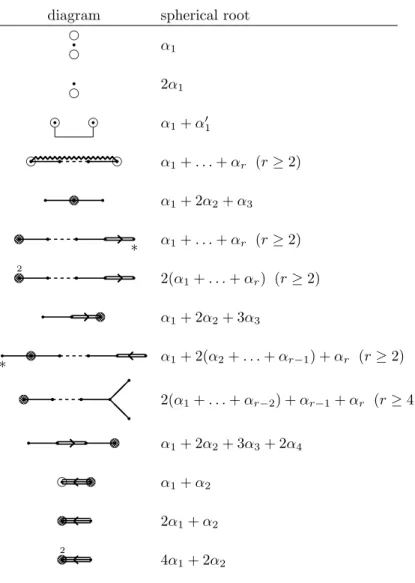
Each spherical root σ ∈ Σ(X) is a linear combination of simple roots with rational, non-negative coefficients (see [Lu01]), and ifGis adjoint then these linear combinations have integer coefficients, since spherical roots obviously belong to the root lattice in this case. The set of simple roots whose coefficient is positive is called thesupportofσ.
For simplicity we assume thatGis adjoint, and each spherical rootσappearing in this case has its own symbol as in Table 1. This symbol is drawn on the part of the Dynkin diagram ofGcorresponding to the support ofσ. The presence of a given spherical root forces simple roots on its support to move some colors. These colors are then drawn in Table 1, and if in the table no color is explicitly drawn in the vicinity of a simple rootα, thenαmoves no color. This rule has actuallytwo exceptions:
(1) in the sixth case, the spherical rootα1+. . .+αr with support of typeBr,
the simple rootαrmay move colors,
(2) in the ninth case, the spherical root α1+ 2(α2+. . .+αr−1) +αr with
support of typeCr, the simple root α1 may move colors.
In the table we mark these exceptions with an asterisk, which is however not re-produced in the actual Luna diagram.
These remarks amount to the compatibility conditions betweenα∈Sp(X) and σ∈Σ(X) mentioned in Remark 5.9, in the case whereαis in the support ofσ. If this is not the case, the only compatibility condition is the one given in Lemma 5.4. Notice that some of the symbols of the table are realized simply by filling the circle corresponding to some colorD moved by a simple rootα in the support of the spherical root. If a color does not constitute in this way the symbol of some spherical root, it is drawn not filled.
We also precise that a “zigzag” line appearing as the fourth case (the spherical
rootα1+. . .+αr, whereα1, . . . , αrform a subdiagram of typeAr) is meant in our
convention to join the two verticesα1,αr, not the two circles drawn around them.
The two circles correspond to two different colors.
Much of the Cartan pairing is often deduced from Proposition 5.6, therefore only in specific situations we need to add some indications about it to the Luna diagram. Following the proposition, the value ofc(D,−) for a colorD moved by a simple root αis entirely determined byα, unless α∈Σ(X). Even in this case, whereα moves the two colorsDα+, D−α, it is enough to give the Cartan pairing for only one
of them, sincec(D±α,−) =α∨−c(D∓α,−). Finally, the value c(Dα±, σ) is positive
for someσ ∈Σ(X) if and only if it is equal to 1, the spherical rootσ is a simple root, andD±
α also appears asD±σ. Hence such values are deduced from the Luna
diagram as we have described it so far.
It remains to include some indications on the valuec(Dα±, σ) in the cases where it is not positive andhα∨, σi 6= 0. In these cases we indicate the valuec(D±
α, σ) =k
by drawing−ksmall arrows on the side of one of the circles representing the color, pointing at some simple root in the support ofσ. We remark that negative values smaller than−1 are possible, as shown in Example 5.7.
A common practice in the literature is to draw these arrows only for the colorD+
α
(the one drawn aboveα), since this is enough to determine the value of the Cartan pairing forD−α, as we have already observed. We will follow this convention here, but we point out that it is then slightly more cumbersome to recognize whether two different Luna diagrams (with equal Σ and ∆) give the same Cartan pairing or not. For this reason, indications for both colors are found in some references.
Example 6.1. For any spherical root of Table 1, one can find a description of the
open G-orbit of the corresponding wonderful variety in [Wa96, Table 1]. Here we
have already seen the casesα1 and 2α1 forG= SL(2) in Example 5.5. Let us see some more cases.
(1) The varietyX =P(Cn+1)×
P((Cn+1)∗), under the diagonal action ofG=
SL(n+ 1), is the wonderful completion of the homogeneous space SL(n+ 1)/GL(n) and has spherical rootα1+. . .+αn.
(2) The variety X =P(V), whereV is the irreducible 8-dimensional
Spin(7)-module, is wonderful under the action of SO(7), and has spherical root α1+ 2α2+ 3α3.
(3) The varietyX =P(U), whereU is the irreducible 7-dimensional G2-module,
is wonderful under the action of G2, and has spherical root 4α1+ 2α2.
Example 6.2. (1) Partial flag varietiesG/P withP ⊇Bdon’t have spherical roots, and their colors are the Schubert divisors. The Luna diagram is therefore given only drawing a circle around each simple root that moves some Schubert divisor. For example, let G be SL(4) with simple roots
Table 1. Diagrams of spherical roots
diagram spherical root
qe e α1 qe 2α1 eq eq α1+α0 1 q qq qq q q q q q e e ppppppppppppppppppppppppppppppppppppppppppppppppppppppppppppppppppppppppppppppppppppppppppppppppppppppppppppppppppppppppppppppppppppppppppppppppppppppppppppppppppppppppppppppppppppppppppppppppppppppppppppppppppppppppppppppppppppppppppppp ppppppppppppp α1+. . .+αr (r≥2) e ppppppppppppppppppppp q qq q α1+ 2α2+α3 q qq qq qq pppppppppppppppppppp q e ppppppppppppppppppppp ∗ α1+. . .+αr (r≥2) q qq qq qq pppppppppppppppppppp q e ppppppppppppppppppppp 2 2(α1+. . .+αr) (r≥2) q qq pppppppppppppppppppp pppppppppppppppppppppqe α1+ 2α2+ 3α3 q pppppppppppppppppppppqqe qq qq q pppppppppppppppppppp q ∗ α1+ 2(α2+. . .+αr−1) +αr (r≥2) e pppppppppppppppppppppq qq qq q q q @@ 2(α1+. . .+αr−2) +αr−1+αr (r≥4) q qq pppppppppppppppppppp qq pppppppppppppppppppppeq α1+ 2α2+ 3α3+ 2α4 q pppppppppppppppppppp pppppppppppppppppppppqe e α1+α2 q pppppppppppppppppppp q e ppppppppppppppppppppp 2α1+α2 q pppppppppppppppppppp q e ppppppppppppppppppppp 2 4α1+ 2α2
α1, α2, α3. The Luna diagram ofX =G/Bis
qe qe qe
Let P be the parabolic subgroup of SL(4) containing B and with Levi subgroup having only the simple rootα3. Then the Luna diagram ofX0=
G/P is e e q q q (2) The diagram qee q q e e
represents the set of spherical roots {α1+α3, α2}, and the set of colors {D, D+
α2, D
−
α2}with Cartan pairing
α1+α3 α2 D 2 −1 D+ α2 −1 1 Dα− 2 −1 1 (3) The diagram q q e e ppppppppppppppppppppppppppppppppppppppppppppppppppppppppppppppppppppp pppppppppppppqeppppppppppppppppppppppppppppppppppppppppppppppppppppppppppppppppppppp pppppppppppppqepppppppppppppppppppppppppppppppppppppppppq pppppppppppppppppppppppppppp pppppppppppppqqeppppppppppppppppppppppppppppppppppppppppppppppppppppppppppppppppppppp ppppppppppppppppppppppppppppppppppeqqe pppppppppppppppppppp qqee
(for G of type Bn) represents the set of spherical roots {α1+α2, α2+
α3, . . . , αn−2+αn−1, αn−1+αn, αn}. Any color takes the values of some
simple coroot, except forD+
αn, D
−
αn, which take the following values:
α1+α2 . . . αn−3+αn−2 αn−2+αn−1 αn−1+αn αn
D+
αn 0 . . . 0 −1 0 1
D−αn 0 . . . 0 −1 0 1
Notice that c(D±αn, αn−1+αn) = 0 because if one of these values were
non-zero, one would be strictly positive (sincehα∨
n, αn−1+αni= 0), con-tradicting Proposition 5.6. (4) The diagram q qq qq q qe e qe e qe e e
forG= SL(5) with simple rootsα1, . . . , α4represents Σ(X) ={α1, α2, α4} and ∆(X) ={D+ α1, D − α1=D − α4, D + α2=D + α4, D −
α2} with Cartan pairing
α1 α2 α4 D+α1 1 0 −1 D− α1 1 −1 1 D+ α2 −1 1 1 D−α 2 0 1 −1 7. Morphisms
In [Kn91] dominant morphisms with connected fibers between spherical varieties are studied. The special case of morphisms between wonderful varieties was derived from loc.cit. in [Lu01]. We report this case in this section.
Let X be a wonderful variety. Recall that we have defined the convex cone V generated inside N = HomZ(Ξ(X),Z) by the elements −σ∗1, . . . ,−σr∗, where
σ∗1, . . . , σ∗r is the dual basis of Σ(X).
Definition 7.1. LetX be a wonderful variety with openG-orbitG/H. IfK is a subgroup ofGcontaining H, we denote by ∆K the set of colors of G/H mapped
dominantly to G/K by the natural map G/H → G/K, and CK the subset ofN
consisting of all elements vanishing onB-eigenvalues ofB-eigenvectors inC(G/K).
Definition 7.2. Let C be a vector subspace of N, and ∆0 ⊆ ∆(X). The couple (C,∆0) is acolored subspace(ofN) ifC is generated, as a convex cone, by finitely
Theorem 7.3([Kn91]). LetXbe a wonderful variety with openG-orbitG/H. The map K7→(CK,∆K)is a bijection between the set of subgroupsK of Gcontaining
H such thatK/H is connected, and the set of colored subspaces ofN. Moreover,K has finite index inNG(K)if and only if the image ofV inN/CK is strictly convex.
Definition 7.4. A subset ∆0⊆∆(X) isdistinguishedif−V intersects the relative interiorE0 of the coneE generated by the elementsc(D,−) forD∈∆0.
Lemma 7.5. Let F1 and F2 be polyhedral convex cones in a finite-dimensional rational vector space. The convex cone generated byF1 andF2 is a vector subspace if and only if the relative interiors of −F1 and ofF2 intersect.
Proof. If the relative interior of−F1 and ofF2 intersect, then the convex cone R generated by F1 and F2 contains the two vector subspaces generated resp. by F1
andF2. It follows thatRis the vector subspace generated byF1together withF2.
Vice versa, suppose thatR is a vector subspace, and consider a point xin the relative interior of −F1. Thenx∈R, so it is a sumx=f1+f2 wherefi ∈Fi for
alli∈ {1,2}. The pointf2 =x−f1 is in the relative interior of−F1, and also in
F2.
By symmetry, we also have that−F1 intersects the relative interior ofF2, letz be a point in this intersection. Ifz=f2 then we are done, otherwise any point on the segment joiningf2andz(possibly except for the endpoints) lyes in the relative
interiors of−F1 and ofF2.
Proposition 7.6 ([Lu01]). Let X be a wonderful variety with open G-orbit G/H, and ∆0 ⊆ ∆(X). Then ∆0 is distinguished if and only if there exists a unique vector subspaceC of N such that(C,∆0)is a colored subspace, and the image ofV inN/CK is strictly convex.
Proof. First we notice that, ifC is a vector subspace ofN, the image of V inN/C is strictly convex if and only ifC ∩(−V) is a face of−V.
Now assume that there exists a colored subspace (C,∆0) ofN such thatC ∩(−V) is a faceFof−V. Denote as above byEthe cone generated by the elementsc(D,−) forD∈∆0, andE0the relative interior ofE. ThenF generatesCas a convex cone together withE, which implies that−F intersectsE0 by Lemma 7.5. Hence ∆0 is distinguished.
Vice versa, suppose that ∆0 is distinguished, so−E
0 intersectsV. Suppose that there exist two faces F1, F2 of V such that their relative interiors intersect −E0. Then the relative interior of the face ofV generated by F1 andF2 also intersects −E0.
It follows that there exists a unique maximal faceF of V such that its relative interior intersects −E0. Then F and E generate a vector subspace C of N by Lemma 7.5.
Finally, we prove the uniqueness of C. Let (C0,∆0) be a colored subspace such
that C0 ∩V is a face F0 of V. Since C0 contains −E0, we have that F0 contains
−E0∩V, which intersects the relative interior ofF. It follows thatF0 containsF. On the other hand,F0 andE generateC0 as a convex cone, which implies that the
relative interior ofF0 intersects −E0. By maximality of F, we have F =F0 and C=C0.
Example 7.7. The set of all colors ∆(X) is always distinguished. One can prove this fact by noticing that ∆(X) is the subset of colors ∆G corresponding to the
inclusionH ⊆G. A combinatorial proof, due to P. Bravi, goes as follows. Thanks to Proposition 5.6, the convex coneEcorresponding to ∆(X) contains the restrictions α∨|Ξ(X) for all α∈ SrSp(X). Therefore there exists an elementxof E that is
strictly positive on all simple roots not inSp(X). As one can check in Table 1, this implies thatxis strictly positive on all elements of Σ(X).
As discussed in details in [Lu01], some subgroups K ⊇ H (such that K/H is connected) are such that G/K admit a wonderful completion Y. A necessary condition recalled in Theorem 4.3 is thatKhas finite index in its normalizer, and a remarkable theorem by Bravi (see [B13]) implies that this condition is also sufficient. We end this section reporting on this result, and on the determination of the spherical roots ofY done by Luna in [Lu01].
Definition 7.8. A distinguished subset of colors ∆0⊆∆(X) isgoodif the monoid
{σ∈spanNΣ(X)|c(D, σ) = 0 for allD∈∆0}
is free. If this is the case, we denote by Σ(X)/∆0 the basis of this monoid.
Proposition 7.9([Lu01]). Let∆0⊆∆(X)be a good distinguished subset of colors, andK⊇H the corresponding subgroup ofG. ThenG/K admits a wonderful com-pletion Y. Moreover, the natural morphism G/H →G/K extends to a surjective equivariant mapX →Y with connected fibers, and we have
Σ(Y) = Σ(X)/∆0
The set of colors ofY in the above proposition is also denoted by ∆(X)/∆0. Theorem 7.10([B13]). All distinguished subsets of colors are good.
We may collect the above results in the following.
Corollary 7.11. LetX be a wonderfulG-variety. The map defined in Theorem 7.3 induces a bijection between the set of surjective, equivariant morphisms with con-nected fibers from X to another wonderful variety and the set of distinguished sub-sets of∆(X).
Example 7.12. (1) The Luna diagram
q q
e e
ppppppppppppppppppppppppppppppppppppppppppppppppppppppppppppppppppppp pppppppppppppqeppppppppppppppppppppppppppppppppppppppppppppppppppppppppppppppppppppp pppppppppppppqe
for G= SL(4) with simple rootsα1, α2, α3, represents the spherical roots Σ(X) = {α1 +α2, α2 +α3} and the colors ∆(X) = {D1, D2, D3} with Di=α∨i|Ξ(X)for alli∈ {1,2,3}. The Cartan pairing is therefore
α1+α2 α2+α3
D1 1 −1
D2 1 1
D3 −1 1
Let us choose Sp(4)⊂SL(4) in such a way that Sp(4)∩Bis a Borel subgroup of Sp(4). Then the above Luna diagram corresponds to the wonderful completionX of the homogeneous space SL(4)/H, whereHis the parabolic subgroup of Sp(4)·Z(SL(4)) containing Sp(4)∩Band corresponding to the long simple root. The subset ∆0 = {D
1, D3} is distinguished, and the monoid {σ ∈spanNΣ(X)| c(D, σ) = 0 for allD ∈ ∆0} is free, with basis
the sumα1+ 2α2+α3 of the two spherical roots ofX. The corresponding surjective equivariant morphismX →Y corresponds to the inclusion H⊂ K= Sp(4)·Z(SL(4)), andY has Luna diagram
e ppppppppppppppppppppp q qq q
(2) The Luna diagram
q qq qq q qe e qe e qe e e
corresponds to the subgroupH ⊆SL(5) of the matrices of the form
λ1A 0 ∗ 0 λ2 ∗ 0 0 λ3A
where A ∈ SL(2) and λ1, λ2, λ3 ∈ C∗ satisfy λ21λ2λ23 = 1. The subset of colors ∆1 ={D−α1, D
+
α2} is distinguished. The quotients Σ(X)/∆1 and ∆(X)/∆1are represented by the Luna diagram
q qq q q q
e e
ppppppppppppppppppppppppppppppppppppppppppppppppppppppppppppppppppppp ppppppppppppp e
and correspond toK1⊃H of the matrices of the form
λ1A 0 ∗ 0 λ2 ∗ 0 0 λ3B
where B ∈ SL(2). Also the subset of colors ∆2 = {Dα+1, D +
α2} is distin-guished, and gives
q qq qq q
e e e e
which corresponds toK2⊃H of the matrices of the form
λ1A ∗ ∗ 0 λ2 ∗ 0 0 λ3A 8. Minimal morphisms
Let X be a wonderful G-variety with open G-orbitG/H. Minimal non-empty distinguished subsets of ∆(X) correspond to subgroups K ⊆Gsuch thatK )H
and K/H is connected, G/K has a wonderful completion Y, and K is minimal with respect to these properties. We may assume that it has a Levi subgroupLK
containing a Levi subgroupLH ofH.
Such subgroups K have been used crucially in the classification of wonderful varieties. Indeed, they are involved in one of the key technical steps both of the uniqueness part of the classification (see [Lo09]), and of the existence part (see [BP14, Section 5.3]). In both parts, loosely speaking, the approach is to use in-duction (e.g. on the dimension ofG/H), showing existence and uniqueness (up to
conjugation) of a subgroup H corresponding to some data Sp(X), Σ(X), ∆(X), assuming them forK and the dataSp(Y), Σ(Y), ∆(Y).
This approach is effective under an additional fundamental assumption: that K and L have the same Levi subgroup, possibly up to some C∗-factors, and that
Ku
)Hu (see case (L) of Proposition 8.1 for a precise statement).
This suggests the importance of distinguishing between different types of inclu-sions K ) H, according to the behavior of Levi subgroups and of the unipotent radicals ofK andH, and motivates Proposition 8.1 below.
Proposition 8.1 ([BL11]). Under the above assumptions, the groups H and K satisfy one of the following statements.
(P) We haveHu)Ku. In this caseH is a maximal proper parabolic subgroup
of K, andZ(LH)◦)Z(LK)◦.
(R) We haveHu=Ku. In this case Hr=Kr, andH/Hr is very reductive in
K/Kr.
(L) We have Hu
(Ku. In this caseLK =LHZ(H)◦ andZ(LH)◦⊆Z(LK)◦,
andKu/Hu isL
H-equivariantly isomorphic to a simpleLH-module.
In the above proposition, we also say that the inclusionH ⊂K isof type(P), (R), or (L), according to which of the statements holds.
The following corollary follows immediately. We recall that thedefectd(X) of a wonderful varietyX is defined asd(X) =|∆(X)| − |Σ(X)|.
Corollary 8.2. Denote byY the wonderful completion ofG/K. Then the following hold.
(1) If d(X)< d(Y)then the inclusion H ⊂K is of type (L).
(2) If the inclusion is of type (R) then d(X) =d(Y). (3) The inclusion is of type (P) if and only ifd(X)> d(Y).
Example 8.3. (1) The subset ∆0of Example 7.12(1) gives an inclusionH⊂K of type (P), and the subset ∆2 of Example 7.12(2) gives an inclusion H ⊂K2 of type (R).
(2) The subset ∆1 of Example 7.12(2) gives an inclusionH ⊂K1of type (L). Notice that here Z(LH)◦ = Z(LK1)
◦, showing that parts (1) and (2) of
Corollary 8.2 are not equivalences in general.
(3) An example whereZ(LH)◦ (Z(LK)◦is the one discussed in Example 5.7.
Let us discuss the caseG= SL(4), which has Luna diagram
q qq q qe e qe e qe e
We can describeH as the subgroup of matrices of the form
λ1 a1 ∗ ∗ 0 λ2 a2 ∗ 0 0 λ3 a3 0 0 0 λ4
where a1, a2, a3 ∈C satisfya1+a2+a3= 0, and λ1, . . . , λ4 ∈C∗ satisfy
λ1· · ·λ4 = 1 and also λ1/λ2 =λ2/λ3 =λ3/λ4. Notice that one can also take another linear combination ofa1, a2, a3(with coefficients all non-zero) instead ofa1+a2+a3, and obtain a subgroup of SL(4) conjugated toH.
The subset of colors ∆0 = {D+1 = D+2 = D+3} is distinguished, and the corresponding subgroup is K = B. Here the inclusion H ⊂ K is of type (L) and we have Z(LH)◦ (Z(LK)◦. In this situation observe that
Z(LK)◦does not normalizeH, in accordance with Theorem 4.3. More
pre-cisely, the unipotent radicalHuis not stable under conjugation byZ(L K)◦,
because it contains a submodule ofKuthat is “diagonal” in a sum ofL K
-submodules contained inKu, all isomorphic as (L◦
K, L◦K)-modules but not
asLK-modules.
References
[Ah83] D.N. Ahiezer,Equivariant completions of homogeneous algebraic varieties by homogeneous divisors, Ann. Global Anal. Geom.1(1983), no. 1, 49–78.
[Av15] R. Avdeev,Strongly solvable spherical subgroups and their combinatorial invariants, Se-lecta Math. (N.S.)21, no. 3, (2015), 931–993.
[B13] P. Bravi,Primitive spherical systems, Trans. Amer. Math. Soc.365(2013), 361–407. [BL11] P. Bravi, D. Luna,An introduction to wonderful varieties with many examples of type F4,
J. Algebra329(2011) 4–51.
[BP14] P. Bravi, G. Pezzini,Wonderful subgroups of reductive groups and spherical systems, J. of Algebra409(2014), 101–147.
[BP16] P. Bravi, G. Pezzini,Primitive wonderful varieties, Math. Z.282(2016), no. 3-4, 1067– 1096.
[Br88] M. Brion,On spherical varieties of rank one (after D. Ahiezer, A. Huckleberry, D. Snow), Group actions and invariant theory (Montreal, PQ, 1988), CMS Conf. Proc., 10, Amer. Math. Soc., Providence, RI, 1989, 31–41.
[Br89] M. Brion, Groupe de Picard et nombres caract´eristiques des vari´et´es sph´eriques. Duke Math. J.58(1989), no. 2, 397–424.
[Br90] M. Brion,Vers une g´en´eralisation des espaces sym´etriques, J. Algebra134(1990), no. 1, 115–143.
[Br07] M. Brion,Log homogeneous varieties, Actas del XVI Coloquio Latinoamericano de ´Algebra, 1-39, Revista Matem´atica Iberoamericana, Madrid, 2007.
[BLV86] M. Brion, D. Luna, Th. Vust,Espaces homog`enes sph´eriques, Invent. Math.84(1986), 617–632.
[BrPa87] M. Brion, F. Pauer, Valuations des espaces homog`enes sph´eriques, Comment. Math. Helvetici62(1987), 265–285.
[DP83] C. De Concini, C. Procesi,Complete symmetric varieties, Invariant theory (Montecatini, 1982), Lecture Notes in Math., 996, Springer, Berlin, 1983, 1–44.
[Kn91] F. Knop.,The Luna-Vust theory of spherical embeddings, Proceedings of the Hyderabad Conference on Algebraic Groups (Hyderabad, 1989), 225–249, Manoj Prakashan, Madras, 1991.
[Kn96] F. Knop,Automorphisms, root systems, and compactifications of homogeneous varieties, J. Amer. Math. Soc.9(1996), no. 1, 153–174.
[Kn14] F. Knop,Spherical roots of spherical varieties, Ann. Inst. Fourier (Grenoble)64(2014), 2503–2526.
[KKV89] F. Knop, H. Kraft, Th. Vust,The Picard group of aG-variety, Algebraische Transfor-mationsgruppen und Invariantentheorie (H. Kraft, P. Slodowy, T. A. Springer, eds.), DMV Seminar, vol. 13, pp. 77–88, Birkh¨auser, Basel-Boston-Berlin, 1989.
[Lo09] I. Losev,Uniqueness property for spherical homogeneous spaces, Duke Mathematical Jour-nal147(2009), no. 2, 315–343.
[Lo09b] I. V. Losev,Demazure embeddings are smooth, Internat. Math. Res. Notices (2009), no. 14, 2588–2596.
[Lu73] D. Luna,Slices ´etales, M´emoires de la S.M.F.,33(1973), 81–105.
[Lu96] D. Luna,Toute vari´et´e magnifique est sph´erique, Transform. Groups1(1996), no. 3, 249– 258.
[Lu97] D. Luna,Grosses cellules pour les vari´et´es sph´eriques, Algebraic groups and Lie groups, Austral. Math. Soc. Lect. Ser., 9, Cambridge Univ. Press, Cambridge, 1997, 267–280.
[Lu01] D. Luna,Vari´et´es sph´eriques de typeA, Inst. Hautes ´Etudes Sci. Publ. Math.94(2001), 161–226.
[MJ88] L. Moser-Jauslin,Some almost homogeneous group actions on smooth complete rational surfaces, L’Enseignement Math´ematique34(1988), 313–332.
[Pe09] G. Pezzini, Automorphisms of wonderful varieties, Transform. Groups14(2009), no. 3, 677–694.
[Se51] J. G. Semple,The variety whose points represent complete collineations ofSronSr0, Univ.
Roma, Ist. Naz. Alta Mat. Rend. Mat. e Appl. (5)10(1951), 201–208.
[Su74] H. Sumihiro,Equivariant completion, J. Math. Kyoto Univ. 14 (1974), 1–28.
[Wa96] B. Wasserman,Wonderful varieties of rank two, Transform. Groups1(1996), no. 4, 375– 403.
To the referee
I thank the referee for the careful reading and many remarks. All comments of the report have been taken into account, here are some details:
(1) I have added some examples where requested.
(2) I have now drawn Luna diagrams always following a common practice, which is to omit the small “arrows” on the side of colors drawn below a simple root (I was not consistent on this in the first version). A comment on this has been added to the description of Luna diagrams before Example 6.1. (3) I have corrected small errors in Remark 3.10 and Example 3.11.
(4) I have expanded the last statement of the first version of the paper, and made it into a couple of paragraphs on the proof of the classification, at the beginning of Section 8.
Dipartimento di Matematica “G. Castelnuovo”, Universit`a di Roma “La Sapienza”, Piazzale Aldo Moro 5, 00185 Roma, Italy