Performance Analysis on Stereo Matching Algorithms Based on Local and Global Methods for 3D Images Application

Performance Analysis on Stereo Matching

Algorithms Based on Local and Global Methods for

3D Images Application

Nurulfajar Abd Manap, Siti Farah Hussin, Abd Majid Darsono, Masrullizam Mat Ibrahim

Innovation (CETRI), Fakulti Kejuruteraan Elektronik Dan Kejuruteraan Komputer (FKEKK), Universiti Teknikal Malaysia Melaka (UTeM), Melaka, Malaysia

[email protected]

Abstract—Stereo matching is one of the methods in computer vision and image processing. There have numerous algorithms that have been found associated between disparity maps and ground truth data. Stereo Matching Algorithms were applied to obtain high accuracy of the depth as well as reducing the computational cost of the stereo image or video. The smoother the disparity depth map, the better results of triangulation can be achieved. The selection of an appropriate set of stereo data is very important because these stereo pairs have different characteristics. This paper discussed the performance analysis on stereo matching algorithm through Peak Signal to Noise Ratio (PSNR in dB), Structural Similarity (SSIM), the effect of window size and execution time for different type of techniques such as Sum Absolute Differences (SAD), Sum Square Differences (SSD), Normalized Cross Correlation (NCC), Block Matching (BM), Global Error Energy Minimization by Smoothing Functions, Adapting BP and Dynamic Programming (DP). The dataset of stereo images that used for the experimental purpose is obtained from Middlebury Stereo Datasets.

Index Terms—Stereo matching; Disparity depth; Dynamic Programming; 3D imaging.

I. INTRODUCTION

Stereo matching of image and video processing is one of the most important studies in stereo vision. Nowadays, there are many studies that have been conducted on the stereo matching algorithm. One of the most widely studied regarding the stereo matching that has been used as a reference is the Scharstein and Szeliski (2001) [1], that categorizes the performance of the algorithm into several categories in terms of method, matching cost, aggregation, optimization and also some important parameters that are often used in the study of the stereo matching. In addition, it also provides quantitative comparisons between stereo matching algorithms. The stereo matching method is divided into two classes, correlation-based algorithms that based on a dense set of correspondences. In other hands, a class that produces sparse algorithm known as Feature-based algorithms. Dense class was divided into two main categories: Local Method and Global Method. There are four steps in the stereo matching algorithm: matching cost computation, cost aggregation, disparity computation and disparity refinement.

Examples of stereo algorithms that implement the Local Methods are Sum Absolute Differences (SAD), Sum Square Differences (SSD), Normalized Cross Correlation (NCC),

Block Matching and Global Error. The characteristics of the Local Method are execution time is shorter, but the value of PSNR and SSIM is very low. Besides that, the Local Method algorithm can only operate on a small window size as the minimum window (1x1) and maximum (25x25), depending on the stereo pair images. Examples of algorithms that comprise the Global Method are Dynamic Programming (DP) and Adapting BP. This method requires long execution time, but the value of PSNR and SSIM is higher. This is because the Global Method involves the process of disparity refinement and disparity optimization. In addition, the Global Method algorithm still provides the highest value of PSNR and SSIM of the window size (25x25).

This research is mainly focusing on performance analysis on the several established stereo matching algorithms and will provide an idea of choosing the better stereo matching algorithms to work on the disparity depth map for the purpose of 3D triangulation applications. The performance on stereo matching algorithm analyzes the Peak Signal to Noise Ratio (PSNR), Structural Similarity (SSIM), the effect of window size and execution time of the Sum Absolute Differences (SAD), Sum Square Differences (SSD), Normalized Cross Correlation (NCC), Block Matching (BM), Global Error Energy Minimization by Smoothing Functions, AdaptingBP and Dynamic Programming (DP). The disparity image is the result of a combination between the first image (the image on the left) and a second image (the image on the right) based on stereo pair images. Images obtained at any of the individual algorithm will be compared with ground truth image. In this research work, the dataset of stereo images are obtained from Middlebury Stereo Datasets developed by Scharstein [1].

II. STEREO VISION

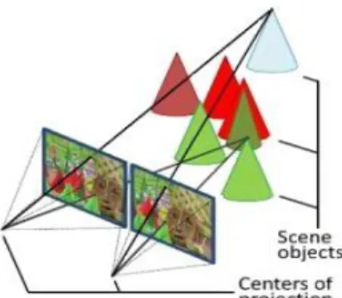
Stereo vision based on triangulation principles used to determine the disparity depth map. This is done by placing two cameras at two different viewpoints (left and right of the image). Figure 1 shows the illustrations of cones from Middlebury Stereo Dataset using the stereo camera. In both images, there are points which connect the surface to the center of each camera projection to form a 3D image. Two steps are performed to obtain 3D images. The first step is to choose whether the reference image, left image or right

image. If the left image was selected, the point of reference needs to be ensured that are identified. Secondly, the position of the camera must be placed exactly. Thus precise geometry can be obtained and will be used to calculate the intersection point of the ray pixels. By assuming the camera left and right once placed, the geometry will be obtained during the calibration process.

Figure 1: Illustrations of scene objects (cones) for left and right of the images by using a stereo camera

The distance between the corresponding pixels of left and the right image is known as disparity [2]. After the disparity values are obtained, the position of the points can be determined by triangulation. However, there are some unwanted aspects such as noise, textureless regions, occluded regions and depth discontinuity regions found during the process in finding the correct values of disparity.

A. Stereo Matching Algorithms

Figure 2 shows the order of the steps for a basic stereo matching algorithm. At the first stage of a stereo matching algorithm, the stereo pair is read as input data for left and right image before proceeding to the next stage. The stereo pair is converted into grayscale images due to single channel images are more efficient in the matching process [3]. Matching cost is the initial step to match the stereo pair and compute the stereo correspondence pixels. There are two categories of matching cost: pixel-based matching cost [4,5,6] and area-based matching cost [7]. After the stereo correspondence pixels obtained, the local support region of matching cost will be summed up by the step on cost aggregation using various type of windows with constant disparity.

Matching cost Cost aggregation Disparity optimization

Disparity refinement

Figure 2: Stereo matching algorithms block

Cost aggregation only works on specified requirements such as an automatically detected window, user-specified orientation window and only pixels inside window [8]. After summation of the cost function, the step of optimization will look for the suitable disparity assignment such as the best area within disparity space image (DSI), which able to reduce the cost functions of an overview on a stereo pair of images. The step of refinement is required to increase the resolution or remove the mismatches due to occlusion [9,10,11]. These are the basic steps of a stereo matching algorithm. However, not all stereo matching algorithms involve the basic steps depending on the design of implementation.

For each pixel in the left image, the pixels on the same scanning line on the right image that captured at the same point can be identified through the matching algorithm. The pixel values are not discriminating in nature, so as a solution using a smaller window size as (5x5 pixels). Line by line will be checked, but only the pixels that are on the left side of the vertical coordinate will be taken into account. If a good and unique pixel was found, the left image pixels are matched with the right image pixels and form a depth map as shown in Figure 3. These stereo matching techniques are known as a local method because it uses only the matching pixel information between the left and right images. However, the weaknesses of the local method provide a low value in areas with poor or repetitive textures as this may prevent to find a good match.

Another method is known as a global method. This method also uses image matching techniques between left and right images either individually or as a group. However, by using this method, the matching process will be faster because this technique does not make an image matching in groups or separately, these techniques will make an overall matching pixel. It will produce a more accurate depth map approach ground truth, but complex algorithm and the processing time are much higher than the Local Method.

(a) (b) (c)

Figure 3: Stereo image matching: (a) The disparity map (ground truth); (b)Left image of ‘Cones’; (c)Right image of ‘Cones’ B. Cost Aggregation Techniques

The efficiency of the matching cost is then improved with summing up the pixels region which from pixel-based matching became area-based matching. Area-based matching is a method, to sum up the matching cost over various type of window with constant disparity value. There are few traditional area-based matching techniques which commonly used for matching cost: sum of absolute differences (SAD), sum of squared differences (SSD), and normalized cross correlation (NCC) [12,13]. SAD is a simple and fast metric method to measure the similarity of two images where it works by subtracting the pixels with a square neighbor pixel between the original image and the target image. Aggregation of the square window is applied on the absolute differences and followed by optimization using winner-take-all (WTA) technique for disparity selection, which shown in Figure 4 [14]. However, this technique has its own limitation where the critical matches only applied for reference image while other points possible get matched with multiple [1]. SSD is slightly different from SAD where the differences between the images are squared and aggregated within the square window and optimized with WTA. SSD has higher complexity than SAD due to its operation of calculation which involved various multiplications. NCC has higher complexity compared to SAD and SSD algorithms as it involves various operations such square root, division and multiplication. There are many other area-based matching algorithms which

developed by other researchers like zero mean normalized cross-correlation [15], gradient-based MF [16], nonparametric [17,18], and mutual information [19].

Figure 4. Pixel-based matching overview

C. Dynamic Programming

Dynamic programming is an approach which frequently used by most researchers to retain stereo correspondence. The dynamic programming on the tree is by applying tree structure of nodes, or the pixels of the image on opposite side of the independent scanlines and only the reliable edges of four linked neighborhood system are selected. Dynamic programming on the tree is an algorithm which considered as a global optimization approach due to disparity estimation at a pixel depends on the estimation at all pixels. Dynamic programming basically is not compatible to a grid of pixels in a graph structure, therefore in this algorithm, the edges with least crucial will be removed till the existing graph becomes a tree then followed by application of dynamic programming upon the resulting tree. The least crucial edges can be described as the edges, which between pixels have less similarity to the same disparity.

In implementation on dynamic programming, the technique used is the pictorial structures for object recognition which developed by [20]. The algorithm of dynamic programming on the tree, the simulation time taken which reduced to O(nh) from O(nh2_{) when a tree contains of}

nodes, n and the number of disparity values as h. The process of reduction is the main complexity of the algorithm.

There are various algorithms which include tree structures as part of their algorithm especially on tree-reweighted message passing for energy minimization [21,22,23]. These algorithms are slightly different from the dynamic programming on the tree as they are used on repetitively passing tree-reweighted messages, and the approach of dynamic programming on the tree is less complexity in computation while efficient algorithm. Dynamic programming on tree algorithm has been evaluated on Middlebury Stereo Vision page and the results are much better than those approaches which based on 1D optimization [24]. The algorithm is also reliable for real-time implementation as it takes about a second for a set of data.

III. PERFORMANCE ANALYSIS

Mühlmann et al. (2002) report that the performance analysis does not perform on the most of the stereo matching algorithm. Therefore, in this paper, the analysis will focus on Peak Signal to Noise Ratio (PSNR in dB), Structural Similarity (SSIM), the effect of window size and execution time for each stereo matching algorithm. The work is based on approximate disparity maps for stereo matching. The analysis of performance for the selected algorithm can be

used to improve the overall performance by adjusting the parameters. Therefore, it will give the insight to the researcher to design better algorithms for specific applications and in order to gain the highest value of PSNR, SSIM and reduce the cost as well as execution time. Therefore, this paper will be discussed on the performance based on these parameters. In this research, the 3x3, 13x13 and 25x25 window size is used. Based on initial results, the small window (3x3) contributes noisy in low texture areas while by using the large window (25x25) the disparity map become blurred at the boundaries.

A. Peak Signal-To-Noise Ratio (PSNR)

PSNR is one of the objective techniques for image assessment and regularly used for the lossy image. Power of signals is in the form of a dynamic range, so the calculation is done on a logarithmic domain. The formula for PSNR stated in Equation (1), MSE MSE PSNR n 2 2 255 log 10 ) 1 2 ( log 10    (1)







where M represents the width and N represent the height, xj,k

the reference image in the grayscale while x’j,k is the

distorted image in the grayscale.

B. Structural Similarity (SSIM)

PSNR used the simple calculations, but is not suitable for some situations and sometimes does not match the Human Visual System (HVS). The SSIM method was proposed by Wang [25] to achieve the correct assessment. This technique is based on the Mean Squared Error (MSE) metric, but the resulting value is close to the Human Visual System (HVS) [26] as given in Equation (3),



where M represents the windows that applied to the frames,

SSIM(x,y) represent the NxM arrays at the luminance channel with the x as the original image while y as the distorted image.

IV. RESULTS AND DISCUSSIONS

The key element of this research is to compare the value of PSNR, SSIM, size of the window, execution time and disparity maps between the local method algorithm and global method algorithm. A stereo matching algorithm with the highest value of PSNR, SSIM, less execution time and a good result in disparity maps for all window sizes is suggested to be used for researchers.

There are three pairs of stereo images that have been used as a data set: Venus, Baby, and Aloe as shown in Figure 5. The three data sets have the different value of maximum disparity (dmax) and characteristics. Performance analysis is conducted on the resulting disparity maps, execution times, the effect of window size, PSNR and SSIM.

Figure 5: Sample of data set and respective ground truth (Venus, Baby and Aloe)

A. Performance Analysis of Execution Time

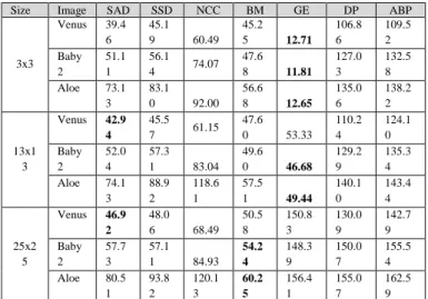
Figure 6 shows the execution time for the window size 13x13. Through observation, for the image pairs Venus, the fastest execution time recorded by Sum of Absolute Difference (SAD) algorithm with a time of 42.94s and the slowest execution time recorded by the AdaptingBP algorithm with a time of 124.10s. As for the image pairs Baby2, the fastest time recorded by the Global Error algorithm with a time of 46.68s while AdaptingBP algorithm recorded the slowest execution time of 135.34s. Aloe image pairs recorded the fastest time of 49.44s by using the Global Error algorithm, and AdaptingBP algorithm takes the longest time to process the image pairs Aloe with a time of 143.44s.

Figure 6: Execution time for window size 13x13

Table 1

Execution Time for window size 3x3, 3x13 and 25x25

Size Image SAD SSD NCC BM GE DP ABP

3x3 Venus 39.4 6 45.1 9 60.49 45.2 5 12.71 106.8 6 109.5 2 Baby 2 51.1 1 56.1 4 74.07 47.6 8 11.81 127.0 3 132.5 8 Aloe 73.1 3 83.1 0 92.00 56.6 8 12.65 135.0 6 138.2 2 13x1 3 Venus 42.9 4 45.5 7 61.15 47.6 0 53.33 110.2 4 124.1 0 Baby 2 52.0 4 57.3 1 83.04 49.6 0 46.68 129.2 9 135.3 4 Aloe 74.1 3 88.9 2 118.6 1 57.5 1 49.44 140.1 0 143.4 4 25x2 5 Venus 46.9 2 48.0 6 68.49 50.5 8 150.8 3 130.0 9 142.7 9 Baby 2 57.7 3 57.1 1 84.93 54.2 4 148.3 9 150.0 7 155.5 4 Aloe 80.5 1 93.8 2 120.1 3 60.2 5 156.4 1 155.0 7 162.5 9

Table 1 presents a summary of the differences in window size on all established algorithm regarding the execution time. The amount of time required for seven established algorithms to process the three image pairs was recorded. Sum of Absolute Difference requires a time of 517.97s, Sum of Squared differences with a time of 575.22s, Normalized Cross Correlation with a time of 762.91s; Block Matching requires a time of 469.37s, Global Error with a time of 642.25s, Dynamic Programming with a time of 1183.79s and AdaptingBP recorded the time of 1244.13s. The total amount of time required for image pairs Venus is 1542.16s, image pairs Baby2 require the total time of 1761.73s, and for the image pairs, Aloe needs as much time as 2091.75s. The overall time required is 5395.65s.

B. Performance Analysis of Peak-Signal-Noise Ratio (PSNR)

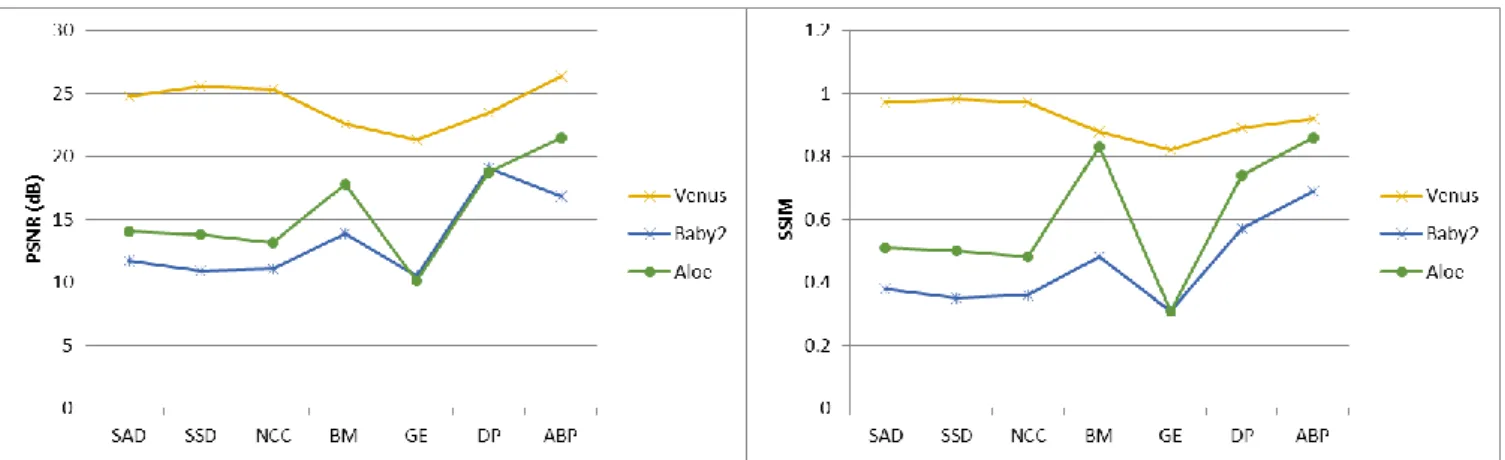
Figure 7 shows the PSNR for the window size 13x13 and Table 2 presents a summary of the differences in window size on all established algorithm regarding the PSNR. Analysis of the window size 13x13 was performed by using the image pairs Venus, Baby2, and Aloe. Through the analysis of the image pairs Venus, AdaptingBP provides the highest PSNR with the value of 26.33dB, while the lowest PSNR recorded by Global Error algorithm with a value of 21.33dB. Image pairs Baby2 recorded the highest PSNR by using a Dynamic Programming algorithm with a value of 19.09dB and the lowest value of PSNR recorded in Global Error with a value of 10.55dB. AdaptingBP recorded the highest PSNR for the Aloe image pairs with a value of 21.46dB and the lowest PSNR recorded in Global Error with the value of 10.12dB.

Figure 7: PSNR for window size 13x13

Table 2

PSNR for window size 3x3, 3x13 and 25x25

Size Image SAD SSD NCC BM GE DP ABP

3x3 Venus 17.27 17.26 14.62 21.76 17.65 19.56 13.72 Baby2 10.22 10.31 11.80 13.74 10.98 15.43 13.91 Aloe 14.48 13.74 12.17 17.23 10.24 16.62 13.35 13x13 Venus 24.74 25.54 25.31 22.60 21.33 23.46 26.33 Baby2 11.69 10.89 11.11 13.87 10.55 19.09 16.85 Aloe 14.05 13.83 13.12 17.79 10.12 18.73 21.46 25x25 Venus 27.51 26.60 26.65 22.97 21.26 28.17 26.58 Baby2 10.81 10.84 12.34 13.51 10.31 13.16 23.53 Aloe 13.51 13.08 12.99 17.54 10.10 19.16 16.88

The amount of PSNR value for seven established algorithms was recorded. Sum of Absolute Difference produced the value of 144.30dB, Sum of Squared differences state the value of 142.09dB, Normalized Cross Correlation with a value of 140.11dB, Block Matching state a value of 161.01dB, Global Error recorded a value of122.53dB, Dynamic Programming with a value of 173.40dB and AdaptingBP recorded the value of 172.59dB. The total amount of PSNR value for image pairs Venus is 470.91dB, image pairs Baby2 recorded the total value of PSNR 274.93dB, and for the image pairs Aloe states the value of PSNR 310.19dB. The overall PSNR value is 1056.03dB.

C. Performance Analysis of Structural Similarity (SSIM)

Figure 8 shows the SSIM for the window size 13x13. Table 3 presents a summary of the differences in window size on all established algorithm regarding the SSIM. An analysis of the window size 13x13 has been made. Through observation, for the image pairs Venus, the highest SSIM recorded by Sum of Square Difference algorithm with a value of 0.98 and the lowest SSIM recorded by the Global Error algorithm witha value of 0.82. As for the image pairs Baby2, the highest SSIM recorded by the AdaptingBP algorithm with a value of 0.69 while Global Error algorithm recorded the lowest SSIM with the value of 0.31. Aloe image pairs recorded the highest SSIM of 0.79 by using the Block Matching algorithm and Global Error algorithm recorded the lowest SSIM with the value of 0.30.

Figure 8: SSIM for window size 13x13

Table 3

SSIM for window size 3x3, 3x13 and 25x25

Size Image SAD SSD NCC BM GE DP ABP

3x3 Venus 0.78 0.77 0.61 0.87 0.78 0.73 0.59 Baby2 0.36 0.36 0.45 0.50 0.31 0.47 0.46 Aloe 0.68 0.71 0.75 0.88 0.32 0.60 0.60 13x13 Venus 0.97 0.98 0.97 0.88 0.82 0.89 0.92 Baby2 0.38 0.35 0.36 0.48 0.31 0.57 0.69 Aloe 0.51 0.50 0.48 0.83 0.31 0.74 0.86 25x25 Venus 0.93 0.93 0.92 0.89 0.81 0.98 0.92 Baby2 0.34 0.35 0.40 0.47 0.30 0.47 0.87 Aloe 0.47 0.45 0.45 0.79 0.30 0.75 0.70

The amount of SSIM value for seven established algorithms was recorded. Sum of Absolute Difference produced the value of 5.42, Sum of Squared differences state the value of 5.38, Normalized Cross Correlation with a value of 5.40, Block Matching state a value of 6.58, Global Error recorded a value of 4.27, Dynamic Programming with a value of 6.20 and AdaptingBP recorded the value of 6.60. The total amount of SSIM value for image pairs Venus is 17.93, image pairs Baby2 recorded the total value of SSIM 9.23 and for the image pairs Aloe state the value of SSIM 12.68. The overall SSIM value is 39.85.

V. CONCLUSION

As a conclusion, the performance of the established stereo matching algorithm in term of Peak Signal to Noise Ratio (PSNR in dB), Structural Similarity (SSIM), the effect of window size and execution time for each stereo matching algorithm has been successfully analyzed. The established stereo matching algorithm was improved by adjusting the parameter value. This research provides an idea of choosing the better stereo matching algorithms to work on the disparity depth map for the purpose of 3D triangulation applications.

ACKNOWLEDGMENT

Authors would like to thank Universiti Teknikal Malaysia Melaka (UTeM) and Ministry of Science, Technology and Innovation (MOSTI) for supporting this research under Science Fund 06-01-14-SF0125 L00026.

REFERENCES

[1] Scharstein, D. & Szeliski, R., 2001. “A Taxonomy and Evaluation of

Dense Two-Frame Stereo Correspondence Algorithms,” 47(1-3), pp.7–42.

[2] Bleyer, M., & Gelautz, M. , 2005. A layered stereo matching algorithm using image segmentation and global visibility constraints.

ISPRS Journal of Photogrammetry and Remote Sensing, 59(3), pp. 128–150.

[3] Koschan, a., Rodehorst, V., & Spiller, K., 1996. Color stereo vision using hierarchical block matching and active color illumination.

Proceedings of 13th International Conference on Pattern Recognition, 1, pp. 835–839.

[4] Donate, A., Liu, X., & Collins, E. G., 2011. Efficient path-based stereo matching with subpixel accuracy. IEEE Transactions on Systems, Man, and Cybernetics, Part B: Cybernetics, 41(1), pp. 183– 195.

[5] Sabatini, M., Monti, R., Gasbarri, P., & Palmerini, G. B., 2013. Adaptive and robust algorithms and tests for visual-based navigation of a space robotic manipulator. Acta Astronautica, 83, pp. 65–84. [6] Jodoin, P. M., Mignotte, M., & Rosenberger, C., 2007. Segmentation

framework based on label field fusion. IEEE Transactions on Image Processing, 16(10), pp. 2535–2550.

[7] Stefano, L. Di, Marchionni, M., & Mattoccia, S., 2004. A fast area-based stereo matching algorithm. Image and Vision Computing, 22(12), pp. 983–1005.

[8] Yang, Q., 2012. A non-local cost aggregation method for stereo matching. 2012 IEEE Conference on Computer Vision and Pattern Recognition, 1, pp. 1402–1409.

[9] Li, G., 2012. Stereo Matching using Normalized Cross-Correlation in LogRGB Space. Computer Vision in Remote Sensing (CVRS), pp. 19– 23.

[10] Fang, L., Li, S., McNabb, R. P., Nie, Q., Kuo, A. N., Toth, C. a., Farsiu, S., 2013. Fast acquisition and reconstruction of optical coherence tomography images via sparse representation. IEEE Transactions on Medical Imaging, 32(11), pp. 2034–2049.

[11] Benzeroual, K., Allison, R. S., & Wilcox, L. M. , 2012. 3D display size matters: Compensating for the perceptual effects of S3D display scaling. IEEE Computer Society Conference on Computer Vision and Pattern Recognition Workshops, pp. 45–52.

[12] Cai, J. , 2007. Fast Stereo Matching : Coarser to Finer with Selective Updating Coarse to Fine Scheme Area-Based Matching. Image and Vision Computing New Zealand, pp. 266–270.

[13] Sinha, S., Scharstein, D., & Szeliski, R., 2013. Efficient High-Resolution Stereo Matching using Local Plane Sweeps. Proceedings of the IEEE Conference on Computer Vision and Pattern Recognition, pp. 1582–1589.

[14] Qin, X., Shen, J., Mao, X., Li, X., & Jia, Y., 2015. Structured-Patch Optimization for Dense Correspondence. IEEE Transactions on Multimedia, 17(3), pp. 295–306.

[15] Almeida, J., Leite, N. J., & Torres, R. D. S. , 2012. VISON: VIdeo Summarization for ONline applications. Pattern Recognition Letters, 33(4), pp. 397–409.

[16] Elboher, E., & Werman, M., 2013. Asymmetric correlation: A noise robust similarity measure for template matching. IEEE Transactions on Image Processing, 22(8), pp. 3062–3073.

[17] Neilson, D., & Yang, Y. H., 2011. A component-wise analysis of constructible match cost functions for global stereopsis. IEEE Transactions on Pattern Analysis and Machine Intelligence, 33(11), pp. 2147–2159.

[18] Mei, X., Sun, X., Zhou, M., Jiao, S., & Wang, H., 2011. 2nd. On building an accurate stereo matching system on graphics hardware.

2011 IEEE International Conference on Computer Vision Workshops (ICCV Workshops), pp. 467–474.

[19] Michael, M., Salmen, J., Stallkamp, J., & Schlipsing, M., 2013. Real-time Stereo Vision : Optimizing Semi-Global Matching. Intelligent Vehicles Symposium (IV), pp. 1197–1202.

[20] Felzenszwalb, P. F., & Huttenlocher, D. P., 2000. Efficient matching of pictorial structures. Proceedings IEEE Conference on Computer Vision and Pattern Recognition. CVPR 2000 (Cat. No.PR00662), 2, pp. 66–73.

[21] Kolmogorov, V., 2006. Convergent tree-reweighted message passing for energy minimization. IEEE Transactions on Pattern Analysis and Machine Intelligence, 28, pp. 1568–1583.

[22] Proenc, H., Neves, C., & Santos, G., 2013. Segmenting the Periocular Region using a Hierarchical Graphical Model Fed by Texture / Shape Information and Geometrical Constraints. IEEE International Joint Conference onBiometrics Compendium, pp. 1-7.

[23] Savic, V., & Zazo, S., 2010. Nonparametric Belief Propagation Based on Spanning Trees for Cooperative Localization in Wireless Sensor Networks. Vehicular Technology Conference Fall (VTC 2010-Fall), 2010 IEEE 72nd, pp. 0–4.

[24] Waggoner, J., Zhou, Y., Simmons, J., De Graef, M., & Wang, S., 2014. Graph-cut based interactive segmentation of 3D materials-science images. Machine Vision and Applications, 25(6), pp. 1615– 1629.

[25] Wang, Z., Bovik, A. C., Sheikh, H. R., & Simoncelli, E. P., 2004. Image quality assessment: from error visibility to structural similarity.

IEEE Transactions on Image Processing : A Publication of the IEEE Signal Processing Society, 13(4), pp. 600–612.

[26] Huat, T.C, Manap, N.A, Ibrahim, MM, 2015, Development of Double Stage Filter (DSF) for Stereo Matching Algorithms and 3D Vision Applications, Journal of Telecommunication, Electronic and Computer Engineering (JTEC), 7(2), pp. 39-46