Predicting Sleepiness from Driving Behaviour
Pablo Puente Guillen
Submitted in accordance with the requirements for the
degree of Doctor of Philosophy.
The University of Leeds
School of Computing
Institute for Transport Studies
School of Psychology
The candidate confirms that the work submitted is his own and that appropriate credit has been given where reference has been made to the work of others.
This copy has been supplied on the understanding that it is copyright material and that no quotation from the thesis may be published without proper acknowledgement.
© 2016 The University of Leeds and Pablo Puente Guillen
The right of Pablo Puente Guillen to be identified as Author of this work has been asserted by him in accordance with the Copyright, Designs and Patents Act 1988.
Acknowledgements
In the present section, an analysis is done to understand the effect different variables had on the completion of the present PhD study. The variables were classified as “academic” and “non-academic”. The “academic” class contained the variables “supervisors” and “colleagues”. It was found that the variable “supervisors” had the biggest effect in the completion of the PhD. The variable “supervisors” were divided in four sub-variables named as following: Professor Anthony Cohn, Professor Oliver Carsten, Dr. Richard Wilkie and Dr. Faisal Mushtaq. Each sub-variable contained a number of attributes: allocation of time, motivation given and idea generation. It was found that the attributes of each sub-variable of “supervisors” were highly correlated with the researcher’s achievements. It was also found that there was a significant effect between the variable “researcher’s incredible gratitude” and the “supervisors” variable. The results led to the conclusion that the completion of the PhD would not have been achieved without the above-mentioned sub-variables.
The second variable contained in the “academic” class was “colleagues”. An experiment was designed by University of Leeds et al. (2012) where multiple participants, hereafter called “students”, were allocated in a confined space for a long period of time. They found that after a certain period of time, which they call “adaptation” period, the participants started interacting with each other, leading to collaboration on each other’s research. It is worth mentioning that several outliers were found. Participants with id tag “Zeynep Uludag” and “David Aguilar Lleyda” presented a higher than “normal collaboration” in the task “completion of PhD experiments” and participants with id tag “Aryana Tavanai”, “Eris Chinellato”, “Panagiotis Spyridakos” and “Daryl Hibberd” presented high collaboration in the task “providing valuable information and Matlab codes”. It was concluded that the collaboration by the “students” has led to a successful completion of the PhD. It is also worth mentioning that a subjective value of “forever grateful” was achieved.
The variable “colleagues” also contained other important sub-variables that affected the completion of the PhD. The sub-variables “Roy Ruddle” and “Natasha Merat” were related to the task “incredible guidance”. The sub-variables “Michael Daly” and “Anthony Horrobin” had a great effect in the task “designing and
developing the experiment”, one of the main tasks in the present PhD study. Using the Karolinska Thankfulness Scale, a value of 10 (“eternally grateful”) was given to each sub-variable.
The “non-academic” class contained very important variables: “family” (parents and brother), “spouse” and “cousins/uncles/aunts/friends”. In accordance to the results found by many other researchers in literature, there is a statistically reliable relationship between “family” and “strength and courage to achieve my goals in life”. The Pearson’s correlation statistic showed a result of 1, reflecting complete dependency between these two measures. In similar way, the variable “spouse” had one of the biggest effects in the overall achievement of the PhD, although from past research, it has been found that the variable “spouse” has been positively related to every achievement of previous endeavours. The so-called “without my spouse I would not be where I am now” coefficient has been and will continue having an effect in future research. Finally, the variable “cousins/uncles/aunts/friends” had a big effect in the task “unwind and relax”, which has led to a value of 10 out of 10 in the Happiness Scale. For further information regarding the sub-variable “cousins/uncles/aunts/friends” please refer to Facebook (Facebook Inc., Cambridge MA, 2014).
The present PhD study was funded by CONACYT. All hail, CONACYT!
A mi abuelita y a nuestros angelitos que nos cuidan todos los dias. Este y cualquier otro logro es gracias a su ayuda.
Abstract
This research investigates the use of objective EEG analysis to determine multiple levels of sleepiness in drivers. In the literature, current methods propose a binary (awake or sleep) or ternary (awake, drowsy or sleep) classification of sleepiness. Having few classification of sleepiness increases the risk of the driver reaching dangerous levels of sleepiness before a safety system can prevent it. Also, these methods are based on subjective analysis of physiological variables, which leads to lack of reproducibility and loss of data, when a lack of consensus is reached amongst the EEG experts. Therefore, the doctoral challenge was to determine whether multiple levels of sleepiness could be defined with high accuracy, using an objective analysis of EEG, a reliable indicator of sleepiness. The study identified awake, post-awake, pre-sleep and sleep as the multiple levels of sleepiness through the objective analysis of EEG. The research used Neural Networks, a type of Machine Learning algorithm, to determine the accuracy of the proposed multiple levels of sleepiness. The Neural Networks were trained using driving and physiological behaviour. The EEG data and the driving and physiological variables were obtained through a series of experiments aimed to induce sleepiness, conducted in the driving simulator at the University of Leeds. As the Neural Network obtained high accuracy when differentiating between awake and sleep and between post-awake and pre-sleep, it led to the conclusion that the proposed objective classification based on objective EEG analysis was suitable. However, this study did not reach the highest levels of accuracy when the 4 levels of sleepiness are combined, nevertheless the solutions proposed by the researcher to be carried in future work can contribute towards increasing the accuracy of the proposed method.
Table of Contents
Acknowledgements ... ii Abstract ... iv Table of Contents ... v Abbreviations ... xii 1. Introduction ... 151.1 Background and research focus ... 15
1.2 Research intent ... 18
1.3 Aims and objectives ... 18
1.4 The thesis structure ... 20
2. Literature review: Sleeping while driving ... 22
2.1 Driving: a complex task ... 22
2.2 Falling asleep while driving ... 24
2.3 The physiology of sleep ... 25
2.3.1 Alertness, drowsiness and sleepiness ... 30
2.3.1.1 Alertness (alert wakefulness) ... 31
2.3.1.2 Drowsiness (quiet wakefulness) ... 31
2.3.1.3 Fatigue ... 32
2.3.1.4 Sleepiness ... 32
2.4 Variables used to predict sleepiness ... 33
2.4.1 PERCLOS ... 33
2.4.2 Driving behaviour ... 34
2.4.3 Physiological variables ... 34
2.4.4 EEG as the ground truth ... 35
2.5 Brain wave and EEG as predictor of sleepiness ... 35
2.6 Differences between young and old drivers ... 39
2.7 Types of automation to prevent sleeping while driving ... 40
2.7.1 Manual driving ... 40
2.7.2 Autonomous cars ... 42
2.7.3 Adaptive automation ... 43
2.8 Conclusion ... 45
3. Literature survey: Classification of sleepiness in drivers ... 48
3.1 Introduction ... 48
3.2 Manual prediction of sleepiness ... 48
3.3 Machine Learning Algorithms ... 50
3.3.1 Definition of Machine Learning Algorithms ... 50
3.3.1.1 Machine and algorithms ... 50
3.3.1.2 Learning ... 51
3.3.2 Evolution of Machine Learning Algorithms ... 53
3.3.3 Types of Machine Learning Algorithms ... 54
3.3.3.1 Supervised learning ... 54
3.3.3.2 Unsupervised learning ... 55
3.3.3.3 Reinforcement learning ... 55
3.4 Machine Learning Algorithms to predict sleep in driving ... 56
3.4.1 Evaluation measures for Machine Learning Algorithms ... 57
3.4.2 Artificial Neural Networks ... 58
3.4.2.1 ANN to predict sleep while driving ... 62
3.4.3 Support Vector Machines ... 63
3.4.3.1 SVM to predict sleep while driving ... 66
3.4.4.1 DBN to predict sleepiness while driving ... 69
3.5 Conclusion ... 72
4. Identifying markers of fatigue in secondary data ... 74
4.1 Introduction ... 74
4.2 Participants and data ... 74
4.2.1 Variables recorded ... 76
4.2.1.1 Target variables ... 77
4.2.1.2 Feature variables ... 81
4.2.2 Statistical Analysis ... 83
4.3 Predicting sleepiness ... 84
4.3.1 Discrete targets using k-Means Clustering algorithm ... 84
4.3.2 Defining a binary levels of sleepiness ... 85
4.3.3 Defining a ternary levels of sleepiness ... 87
4.3.4 Predicting levels of sleepiness using Support Vector Machine ... 89
4.3.5 Predicting levels of sleepiness using Neural Networks ... 91
4.3.6 Continuous target ... 94
4.3.6.1 Radial Basis Function Network ... 94
4.4 Conclusion ... 96
5. Inducing high levels of sleepiness in drivers ... 99
5.1 Introduction ... 99
5.2 Study 1: Effects of lunch on drivers’ sleepiness ... 99
5.2.1 Aims ... 99
5.2.2 Method ... 100
5.2.2.1 Driving simulator ... 100
5.2.2.2 Participants ... 102
5.2.2.3 Design ... 103
5.2.3 Subjective data recording ... 105
5.2.4 Driving data recording ... 106
5.2.5 EEG data recording ... 107
5.2.5.1 Frequency bands ... 108
5.2.5.2 Fast Fourier Transform ... 108
5.2.5.3 Electrode clusters ... 113
5.2.6 Artifacts and automatic cleaning for EEG data ... 114
5.2.6.1 Type of artifacts ... 115
5.2.6.2 EEG cleaning methods ... 118
5.2.6.3 Automatic cleaning method developed in Matlab ... 118
5.2.6.4 Results of automatic cleaning method ... 120
5.2.7 Statistical analysis ... 121
5.2.7.1 Subjective sleepiness results ... 121
5.2.7.2 Driving behaviour results ... 122
5.2.7.3 EEG results ... 125
5.2.8 Study 1: Conclusion ... 128
5.3 Study 2: Effects of a one-hour monotonous driving task on drivers' sleepiness 130 5.3.1 Aims ... 130 5.3.2 Method ... 131 5.3.2.1 Participants ... 131 5.3.2.2 Design ... 131 5.3.3 Statistical analysis ... 134
5.3.3.1 Subjective sleepiness results ... 134
5.3.3.2 Physiological behaviour results ... 138
5.3.4 Study 2: Conclusion ... 140
6. Identifying markers of sleepiness using EEG ... 143
6.2 Determining different levels of sleepiness using EEG and MLA ... 145
6.2.1 Defining binary clusters of sleepiness using EEG ... 147
6.2.2 Predicting binary clusters of sleepiness using driving behaviour ... 151
6.2.3 Predicting multiple clusters of sleepiness using driving behaviour ... 155
6.2.4 Predicting binary clusters of sleepiness using driving and physiological behaviour ... 157 6.3 Conclusion ... 158 7. Discussion ... 160 7.1 Contributions to knowledge ... 160 7.2 Overview ... 161 7.3 Introduction ... 161 7.4 Summary of results ... 163
7.4.1 Dataset 1: Determining the levels of sleepiness using blinking behaviour 163 7.4.2 Sleep inducing experiments ... 166
7.4.3 Dataset 2: Determining the levels of sleepiness using EEG ... 167
7.5 Limitations ... 173
7.5.1 Real world driving versus control environment experiment ... 173
7.5.2 Use of EEG in a real environment ... 173
7.5.3 Individuality of sleepiness patterns ... 174
7.6 Future Directions ... 174
References: ... 177
Bibliography ... 194
Appendix A Consent Form given to the participants during the experiments . 206 Appendix B Debrief Information Sheet (post experiment – after both driving tasks have been completed) ... 207
Appendix C Instruction Sheet for the participants ... 208
Appendix D Karolinska Sleepiness Scale test ... 209
Appendix E Screening Questionnaire for participants ... 210
Appendix F The Epworth Sleepiness Scale (ESS) ... 211
Appendix G Big 5 Personality Scale ... 212
Appendix H BIS-BAS questions ... 214
Appendix I Stress and Arousal Checklist ... 216
Appendix J Perceived Stress Scale ... 217
Appendix K Recruitment poster for Study 1 ... 218
Appendix L Recruitment poster for Study 2 ... 219
Appendix M Examples of correlation analysis of Driving variables and EEG variables for study 1 ... 220
Figure 2-1 Most common road traffic accidents factors according to the European
Truck Accident Causation ... 24
Figure 2-2 Sinusoidal waveform and its components. ... 26
Figure 2-3 Visual representation of different sine waves ... 27
Figure 2-4 Example of brain wave activity recorded from a human participant ... 28
Figure 2-5 Effect of FFT in different sine waves. ... 29
Figure 2-6 Brain wave activity during awake and sleep stages. ... 30
Figure 2-7 EEG net cap with 129 electrodes (used to record brain wave activity) held together with a transparent rubber net. ... 36
Figure 2-8 Depending on the activity, EEG data (brain wave activity) can be classified in different frequency bands. ... 37
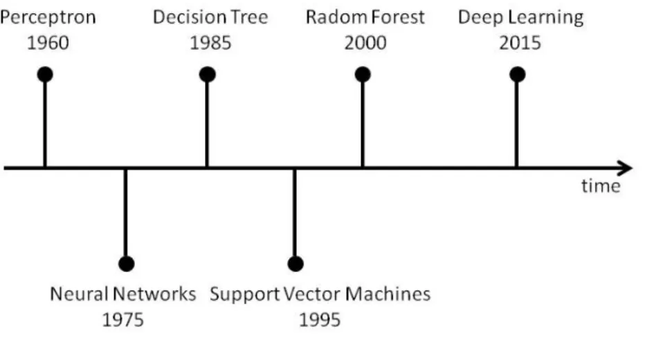
Figure 3-1 Timeline of the development of different MLAs that are still used nowadays ... 53
Figure 3-2 Mathematical model of a neuron produced by McCulloch and Pitts in 1943. ... 60
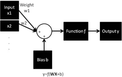
Figure 3-3 Single-input neuron ANN design ... 60
Figure 3-4 Multiple input neuron ANN design ... 62
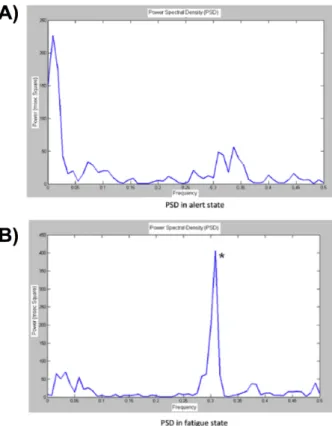
Figure 3-5 Power spectra density of the heart rate variability of “awake” drivers (a) and “sleepy” drivers (b) during a driving simulator study. ... 63
Figure 3-6 Benefits of SVM. ... 64
Figure 3-7 Dataset classified by three different classification lines. ... 64
Figure 3-8 The data points used to determine the maximum space between the linear classifier are called Support Vectors. ... 65
Figure 3-9 Eye blink and brain activity sample used to determine the different stages of sleepiness and train the SVM. ... 67
Figure 3-10 Features extracted from a single blink of a participant to train the SVM. ... 69
Figure 3-11 DBN developed to detect sleepiness states in the driver. ... 71
Figure 4-1 Blinking behaviour variables (PERCLOS, blinking duration and blinking frequency) for the older and young group. ... 80
Figure 4-2 Standard deviation lane position, standard deviation steering and mean steering variables of the older and young group. ... 83
Figure 4-3 Result of the unsupervised k-means algorithm for two clusters using PERCLOS (plotted in the x-axis) and Blinking frequency (plotted in the y-axis) ... 87
Figure 4-4 Result of the unsupervised k-means algorithm for two clusters using PERCLOS (plotted in the x-axis) and Blinking frequency (plotted in the y-axis). ... 89
Figure 4-5 NeuroNets 3 layer feed-forward with 12 hidden layers design used to predict a binary classification of sleepiness ... 92
Figure 4-6 Results of using RBF with four different regularisation parameters using sampled data obtained from a sine wave ... 96
Figure 5-1 a) Motion base driving simulator at the University of Leeds and b) Static driving simulator at the University of Leeds. ... 101
Figure 5-2 EGI system used to record brain wave activity.. ... 105
Figure 5-3 Effect of convolution on a signal.. ... 109
Figure 5-4 Steps to perform a convolution process on a signal ... 110
Figure 5-6 Taper functions for segmentation of a EEG dataset used to reduced the non-stationary problem of EEG signals. ... 112
Figure 5-7 The electrodes' labels and locations on the 128 channel EGI sensor net.114
Figure 5-8 A single electrode EEG recording showing different artifacts ... 115
Figure 5-9 EGI interface which allows to identify electrode whose impedance are above certain threshold. ... 116
Figure 5-10 Cleaning process to remove artifacts automatically developed in Matlab
... 119
Figure 5-11 EEG data removed using manual (red) and automatic cleaning (green) in two random participants ... 121
Figure 5-12 The scores of the KSS test before and after the driving task separated by the lunch condition ... 122
Figure 5-13 Driving variables behaviour separated by lunch condition with error bars representing the standard error.. ... 124
Figure 5-14 Changes in theta, alpha, beta, theta+alphabetaand alphabeta over time for the first study. ... 126
Figure 5-15 Heatmap presenting the correlation analysis between the nine time segments (each time segment represents 5 minutes of the driving task) of SDLP
and alphabeta in the middle parietal region of the head. ... 127
Figure 5-16 Heatmap presenting the correlation analysis between the nine time segments (each time segment represents 5 minutes of the driving task) of SDLP and theta+alphabeta in the middle parietal region of the head. ... 128
Figure 5-17 SmartEyePro camera and their position in the experiment room ... 133
Figure 5-18 MTx device, used to track the head movement, positioned on top of the EEG. ... 134
Figure 5-19 The scores of the KSS (subjective sleepiness) test before and after the driving task ... 135
Figure 5-20 Driving variables behaviour with error bars representing the standard error. ... 136
Figure 5-21 Changes in theta, alpha, beta, theta+alphabetaand alphabeta over time for the second study. ... 137
Figure 5-22 Heatmap presenting the correlation analysis between the twelve time segments (each time segment represents 5 minutes of the driving task) of SDLP
and alphabeta in the middle parietal region of the head for the results obtained
in study 2. ... 138
Figure 5-23 Axis coordinates according to head position of the participants ... 139
Figure 5-24 Heatmap presenting the correlation analysis between the 9 time segments (each time segment represents 5 minutes of the driving task) of the SD of the head movement in y axis and alphabeta in the middle parietal region of the head. ... 141
Figure 6-1 Visual indicators of sleep in EEG data used by clinicians to determine the different sleepiness states. ... 146
Figure 6-2 Topological plot of the mean power of the EEG ratios a) theta+alpha/beta and b) alpha/beta 20 seconds before the participant drove out of the lane. ... 149
Figure 6-3 Mean power of the EEG ratios a) theta+alpha/beta and b) alpha/beta 20 seconds before the participant drove out of the lane per block of the head ... 150
Figure 6-4 NeuroNets 3 layer feed-forward with 7 neurons in the hidden layers design used to predict a binary classification of sleepiness using driving variables as inputs ... 152
Figure 6-5 Sensitivity analysis showing the changes in accuracy as the number of data points increase.. ... 154
Figure 6-6 Results of the k-means clustering algorithm using the EEG ration alpha/beta and KDS of alpha to determine two levels of sleepiness using the “Neither” section. ... 156
Figure 7-1 Flow chart used by Shuyan & Gangtie (2009) to classify the different levels of sleepiness using KSS and KDS. ... 171
Table 3-1 Variables used by Yang, Lin & Bhattacharya (2010) ... 70
Table 4-1 Initial and final distances of each event recorded (the units are in metres). The driving and physiological variables were recorded only during certain
segments throughout the whole driving task. ... 77
Table 4-2 SVM error box using two clustered datasets as targets and driving variables as feature. The columns refer to the target and the rows refer to the prediction . 90
Table 4-3 SVM error box using 2 clustered datasets as targets and the relative value of the driving variables according to baseline as feature ... 91
Table 4-4 NeuroNets error box using 2 clustered datasets as targets and driving
variables as feature ... 93
Table 4-5 NeuroNets error box using 3 clustered datasets as targets and driving
variables as feature ... 94
Table 5-1 Statistical analysis of the effect of drive time in the driving variables ... 136
Table 5-2 Statistical analysis of the effect of drive time in the head movement
variables ... 140
Table 6-1 Ablative analysis to determine the effect each feature has in the accuracy of the overall system ... 154
Table 6-2 Error box to determine the accuracy of the NeuroNets when predicting 2 levels of sleepiness ... 155
Table 6-3 Error box to determine the accuracy of the NeuroNets when predicting 3 levels of sleepiness ... 155
Table 6-4 Error box to determine the accuracy of the NeuroNets when predicting 2 levels of sleepiness within the “Neither” cluster ... 157
Table 6-5 Error box to determine the accuracy of the NeuroNets when predicting 4 levels of sleepiness ... 157
Abbreviations
The following key would be beneficial for decoding the abbreviations used in this thesis.
CAR Center for Automotive Research
ICCT International Council for Clean Transportation NHTSA National Highway Traffic Safety Administration
WHO World Health Organisation
IRTU International Road Transport Union
EEG Electroencephalogram
FFT Fast Fourier Transform
REM Rapid eye movement
fMRI Functional magnetic resonance image fNIR Functional near-infrared spectroscopy
MLA Machine learning algorithm
PERCLOS Percentage of eye closure
ECG Electro-cardiography
RBF Radial Basis Function Network
ESS Epsworth Sleepiness Scale
SDLP Standard deviation of lane position SDSpeed Standard deviation of speed
SDSteering Standard deviation of steering wheel angle
HFS High frequency steering
TTLC Time to lane crossing
OOL Out of lane
EGI Electrical Geodesics Inc.
ICA Independent component analysis
BESA Brain Electrical Source Analysis
CGF Centre of gravity frequency
KDS Karolinska Drowsiness Scale
NASA The National Aeronautics and Space Administration DTREG Nonlinear Regression and Curve Fitting
SMOTE Synthetic Minority Oversampling Technique
RMSE Root mean square error
Chapter 1:
1.
Introduction
1.1
Background and research focus
This thesis describes a programme of research that investigates a solution to determine and predict different levels of sleepiness in drivers using brain wave activity as well as driving and physiological behaviour. The impetus for carrying out this research was an opportunity to develop a solution that could reduce accidents due to falling asleep while driving. Today, there are more than one billion cars circulating around the world and it is expected that this will double during the next decade (Center for Automotive Research, 2011; Dargay et al., 2007; International Council for Clean Transportation, 2014; WHO, 2009; Sperling & Gordon, 2008; Sousanis, 2011). The prevalence of automotive vehicles means that ensuring the safety of drivers, passengers and pedestrian is a top priority for researchers and car manufacturers (Royal, 2003; Philip & Akerstedt, 2006; Maycock, 1997; Horne & Reyner, 1999; NHTSA, 1999). Unfortunately, there are around 50 million road accidents every year and approximately 1.2 million of them result in fatalities (WHO, 2009). From all the road accidents, approximately 85% are accounted to human errors (International Road Transport Union, 2007).
One of the most common and dangerous causes of road accident due to human-error is sleeping while driving (Royal, 2003; Philip & Akerstedt, 2006; Connor et al., 2001; NHTSA, 2015). It has been estimated that, across the world, around 20% of road crashes are related to sleepiness (MacLean et al., 2003). In the U.S.A. alone, around 1,550 crashes due to sleepiness resulted in a fatality per year (NHTSA, 1999). Based on the frequency and magnitude of sleep-related driving errors there has been a push towards exploring ways in which one might be able to predict high levels of sleepiness in the driver to avoid road accidents while driving.
In order to tackle this problem, the first steps taken by a number of researchers and car companies has been to identify the most suitable variables to predict the level of sleepiness in the driver. For example, recently Lexus (2012) presented a device that would determine the level of sleepiness of the driver by analysing their blinking behaviour- as research indicates that longer and more frequent blinks are related to higher levels of sleepiness (Yeo et al., 2009). On the
other hand, Bosch (2012) developed a system that used lateral movement of the car as a determinant of the level of sleepiness.
Although physiological and driving behaviour are highly correlated with sleepiness, electrical activity produced by the brain has been found to be more reliable to determine sleepiness. One of the methods to measure electrical activity produced by the brain is using an electroencephalogram (EEG; electrodes in contact to the scalp of the human). Brain wave activity suffers fewer changes due to changes in the driving environment (Artaud et al., 1994; Lal et al., 2003; Jap et al., 2009). EEG provides a highly reliable biological marker of different levels of physiological arousal (Jap et al., 2009; Lal & Craig, 2001a,b; Stern & Engel, 2005; Yeo et al., 2009; Zhao et al., 2012; Akerstedt & Gillberg, 1990; Campagne, Pebayle & Muzet, 2004; Jap et al., 2009; Kecklund & Akerstedt, 1993; Zhao et al., 2012; Lowden et al., 2009). To separate this EEG activity data into different levels of sleepiness, expert clinicians subjectively classify the data using visual indicators in the brain wave activity data. Unfortunately, when clinicians attempt to classify the data into different levels of sleepiness, many discrepancies arise due to the subjectivity of the visual analysis of the EEG signal (Yeo et al., 2009; Vuckovic et al., 2002; Knoblauch et al., 2003; Andrillon et al., 2011; Benbadis, 2006; Carskadon and Dement, 2011; Gennaro and Ferrara, 2003; Devuyst et al., 2010; Cantero et al., 2002; Parekh et al., 2015; Teplan, 2002). This relatively poor inter-rater reliability decreases the amount of data that can be used to inform sleep-related decisions. By developing an objective analysis of this brain wave activity data, the classification process can be reproduced in any data set without the need to consult clinicians. Such an objective analysis would also reduce the amount of data lost due to a lack of agreement from the clinicians. Therefore, one of the primary goals of this PhD project is to produce an objective analysis of brain wave activity to identify sleepiness.
Once the variables being used to determine the levels of sleepiness have been decided upon, the next step is to determine how to define and predict different levels of sleepiness. Although many researchers and car companies have developed systems to predict and prevent sleepiness, these systems only react to a binary or ternary number of levels of sleepiness (Lal et al., 2003; Sayed & Eskandarian, 2001; Yeo et al., 2009; Shuyan & Gangtie, 2009; Yang et al., 2010; Patel et al., 2011;
NapZapper, 2016; Bosch, 2012; Lexus, 2012), i.e. the sleepiness level changes from “awake” to “sleep” in a binary system and from “awake” to “drowsy” to “sleep” in a ternary system. During the “sleep” level, the driver’s capabilities reduce and the probability of a road accident is high (Royal, 2003; Philip & Akerstedt, 2006; Connor et al., 2001; Klauer et al., 2006; Lamond & Dawson, 1999). This means that when a system that can only determine binary states of sleepiness predicts a “sleep” state, the driver is already in a high risk of being involved in a road accident.
A system with ternary states of sleepiness (awake, drowsy and sleep) allows for smoother and safer transitions between the levels of sleepiness. Once the system has determined the instantaneous level of sleepiness of the driver, the system can take actions to warn the driver (if the level of sleepiness is low) or aid the driver through the automation of certain driving tasks (if the level of sleepiness is high). If the system detects a medium level of sleepiness (“drowsy” state), a low level of automation action, e.g. an alarm suggesting the driver to take a break or coffee, would suffice to alert the driver of the potential danger if he/she continues to drive while his/her level of sleepiness increases. On the other hand, if the system determines a high level of sleepiness, a high level of automation action would be needed from the system, e.g. the car would take partial or complete control of the driving tasks, and this has a high risk of being involved in a road accident. Therefore, reducing or completely removing control of the driving tasks from the driver would reduce the possibility of the driver performing an incorrect driving action. Unfortunately, research found that jumping from a high level of automation action to a low level of automation action has serious consequences on the driver, leading to serious accidents (Merat et al., 2014; Endsley, 1995; Carsten et al., 2012). By determining a higher number of levels of sleepiness, it is possible to have a smoother and safer transition between the levels of automation of the actions required for each level of sleepiness. Therefore, the present PhD study proposed a multiple classification of the levels of sleepiness.
In the present PhD, the researcher explored different algorithms used to determine and predict different levels of sleepiness using physiological and driving behaviour. An understanding of the brain wave activity data as well as the driving and physiological behaviour allowed the adoption of a Machine Learning Algorithm
that could predict and determine the multiple levels of sleepiness aimed to obtain at the end of the present PhD study.
1.2
Research intent
This PhD project presents a novel approach to classifying EEG data analysis. By adopting an objective analysis of the data, it is possible to avoid the problems that arise when analysing the data according to subjective visual interpretation. It also allows for reproducibility and repeatability of the analysis method when the amount of data or the data sets is high.
This PhD also explores the possibility of detecting multiple levels of sleepiness using physiological and driving behavioural data. Using Machine Learning algorithms, analysis was conducted to determine the possibility of creating a system that would predict different levels of sleepiness of a driver and therefore allow different level of action with different levels of automation. It is hypothesised that such system could reduce and prevent accidents related to sleepiness while driving by detecting premature signs of sleepiness and react preventively to avoid any incident.
1.3
Aims and objectives
The intention and purpose of the research was to determine the role that driving and physiological behaviour plays when detecting sleepiness in drivers. The research also seeks to provide a more robust and objective quantification and classification of the brain wave activity data, i.e. the basis for the classification of the sleepiness’ states. By using Machine Learning algorithms, it is possible to determine the accuracy of the different levels of sleepiness classified through brain wave activity as well as the role that each physiological and driving behavioural variable plays when detecting the mentioned levels of sleepiness.
The research in the first year focused on determining the different variables used in research and industry to classify the different levels of sleepiness. An analysis was done to understand the effect of changes in sleepiness on different driving and physiological variables. An analysis was also done on the different Machine Learning algorithms used in research to predict sleepiness using physiological and driving data.
This allowed a better understanding of the design of experiments, in order to obtain sleeping data from participants while driving. Following this first year, the study conducted a number of experiments focused on obtaining physiological and driving data from drivers while their sleepiness increased. These experiments were conducted using a driving simulator to reduce the risks of danger of driving while being in a high state of sleepiness. Finally, the data obtained from the experiments conducted was used to predict the levels of sleepiness through a Machine Learning algorithm. The broad aims are described below followed by the objectives devised to achieve them:
Aim 1: Identifying the literature related to physiological and driving behaviour of people driving under a high state of sleepiness.
• Distinguish how physiological and driving variables are modulated
as sleepiness increases
• Determine the “ground truth” used in literature to classify sleepiness
into different clusters
Aim 2: Provide an objective analysis of the EEG data
• Determine the challenges and advantages of using visual analysis
(subjective) of the brain wave activity data
• Define the variables and factors used as identifiers by clinicians
when visually analysing brain wave activity data
• Develop a reproducible program able to obtain high accuracy when
objectively analysing the brain wave activity data of different participants
Aim 3: Adopt a Machine Learning algorithm to detect multiple levels of sleepiness using the drivers’ data
• Determine the advantages and disadvantages of different Machine
Learning algorithms
• Define the parameters of the algorithm that would achieve the
• Analyse the role of physiological and driving data towards the
detection of the different levels of sleepiness
1.4
The thesis structure
Chapter 1 Introduction: the study’s focus, scope, aims, objectives and significance
Chapter 2 Literature review: Sleepiness while driving: correlation of the study’s central argument and theoretical foundation with existing literature
Chapter 3 Literature review: Classification of sleepiness in drivers: analysis of the different algorithms that have been used in previous research focusing on sleeping while driving
Chapter 4 Identifying markers of sleepiness in secondary data: Data analysis using blinking behaviour as the factor that classifies the levels of sleepiness and driving behaviour as the predictor data. The data used in this chapter was obtained from past research conducted by another researcher in the driving simulator.
Chapter 5 Inducing high levels of sleepiness in drivers: Narrative of the experiment design that was conducted in a static driving simulator during this PhD study to obtain sleep data from participants and the subsequent results.
Chapter 6 Identifying markers of sleepiness using EEG: A Machine Learning algorithm is trained using the driving and physiological data obtained during the experiment conducted presented in Chapter 5. The levels of sleepiness are determined by classifying the brain wave activity into different clusters.
Chapter 7 Discussion and conclusion: Relates the finding from the data analysis to results obtained by other researchers and presents a statement of the contribution the research makes to new knowledge.
Chapter 2:
Literature review: Sleeping
while driving
2.
Literature review: Sleeping while driving
The following chapter starts by discussing the complexity of the driving task and the consequences of human errors (non-performance errors) while driving. One of the most common human errors while driving is sleeping while driving (Internatioanl Road Transport Union, 2007). The chapter further develops the statistics regarding crashes of people falling asleep on the wheel and the different approaches taken to predict and prevent this type of human error. Sleepiness is the major contributor of this type of error. The different stages of sleepiness, as well as its consequences in the physiology of people, are further explained in this chapter. At the end of the chapter, a summary of different types of automation approaches that can lead to a reduction on accidents due to sleepy drivers is presented.
2.1
Driving: a complex task
Driving is an everyday task that allows millions of people around the world to transport themselves and/or goods from one place to another with relative ease. There has been a substantial rise in driving over the past three decades (Grove, 2015; George & Kershaw, 2016; Leibling, 2008). In the United Kingdom alone, the number of vehicles on the road has increased dramatically every year since 1950 and there are now 35.6 million vehicles licensed in total (Grove, 2015; George & Kershaw, 2016). According to research, in 2020 there will be over 37 million vehicles on the road in the United Kingdom (Leibling, 2008). Whilst this appears to be a routine task in many people’s lives, the act of driving is layered with complexity.
A simple model explaining the different levels of complexity present in driving was described in Plankermann (2013). The model is a combination of Michon’s (1985) task hierarchical model and Rasmussen (1983) task performance. The model presents three hierarchical levels (strategic, manoeuvring and control) and each one is associated to a task performance.
(i) The first level is the strategic level (knowledge task). In driving, this first level is associated with the knowledge the driver has of the road, i.e. mental map of the directions to a destination, knowledge of streets, etc.
(ii) The second level is the manoeuvring level (rule task). In driving, this is represented by the knowledge the driver has regarding the driving rules, i.e. distance the driver should maintain with the car in front, speed needed to take a gentle curve, etc.
(iii) The third level is the control level (skill task). This level is how well the driver performs the desired action planned in the manoeuvring level. A failure in any of these levels (human error accident) could lead to a collision that could endanger the people inside and outside the car (National Highway Traffic Safety Administration [NHTSA], 2015).
According to the International Road Transport Union, the number of road freight accidents due to human error is approximately 85% (Figure 2-1) (International Road Transport Union, 2007). In 2009, more than 2,000 people died in the UK due to road traffic accidents (Box, 2011). Although it only represented 0.5% of all deaths in that year, for young people (between 15 and 19 years old) it represented 25% of all deaths (Box, 2011). Crashes due to human error can be categorised in recognition error (strategic level), decision error (manoeuvring level), performance error (control level) and non-performance error (National Highway Traffic Safety Administration [NHTSA], 2015). Non-performance factors (sleep, alcoholic or drug intoxication, etc.), although not that common, can affect the three task hierarchy levels outlined above and thus cause serious accidents (European Agency for Safety and Health at Work [EU-OSHA], 2010). One of the most dangerous and common non-performance errors is sleeping while driving (Royal, 2003; Philip & Akerstedt, 2006; Connor et al., 2001, National Highway Traffic Safety Administration [NHTSA], 2015).
Figure 2-1 Most common road traffic accidents factors according to the European Truck Accident Causation (Adapted from: IRTU, 2007)
2.2
Falling asleep while driving
Sleepiness is one of the major causes of road traffic accidents (Royal, 2003; Philip & Akerstedt, 2006; Connor et al., 2001). MacLean et al. (2003) estimated that, around the world, approximately 20% crashes are related to sleepiness, where off-road crashes, i.e. driving out of the off-road, are the most common (George, 2005). In the United Kingdom 15-20% of the accidents are related to sleepiness (Maycock, 1997; Horne & Reyner, 1999) and in the U.S.A. it is estimated that there are 56,000 sleep-related crashes each year of which 1,550 resulted in a fatality (NHTSA, 1999).
The risk of having an accident while being sleepy is four to six times higher than when the driver is alert (Klauer et al., 2006). Researchers have demonstrated that a driver who has sleep deprivation has the same driving skills as a person with an illegal high concentration of alcohol in their system (0.1 g/l) (Lamond & Dawson, 1999). In order to understand how we might build interventions to address this important topic of research, it is necessary first to examine the physiology of sleep and distinguish the difference between alertness and sleepiness as well as the different “sleep” and “awake” stages before engaging in methods to predict and prevent people from falling asleep while driving.
0.00% 10.00% 20.00% 30.00% 40.00% 50.00% 60.00% 70.00% 80.00% 90.00% 100.00%
Most common road traf<ic accidents
Human Factors Technical Factors Infrastructure Conditions
2.3
The physiology of sleep
According to Sadock and Sadock (2000, p. 281), “sleep is a state of decreased awareness of environmental stimuli that is distinguished from states such as coma or hibernation by its relatively rapid reversibility”. Another important characteristic of sleep is that as sleepiness increases, the individual is capable to recognize higher levels of sleepiness (Sadock & Sadock, 2000; Carskadon & Dement, 2011). In addition, there is a correlation between the feeling of “sleepy” and visible behavioural changes as well as changes in the physiology of the individual (Sadock & Sadock, 2000; Carskadon & Dement, 2011, Boyle et al., 2008; Brookhuis & de Waard, 2010; Filtness, Reyner & Horne, 2012).
The changes in behaviour due to sleepiness have been widely studied in literature (Sadock & Sadock, 2000; Carskadon & Dement, 2011, Boyle et al., 2008; Brookhuis & de Waard, 2010; Filtness, Reyner & Horne, 2012; Jap, Lal & Fisher, 2011). In many studies, it has been found that as sleepiness increases, the blinking behaviour of an individual modifies by an increase in the frequency of blinks, a longer duration of blink and shorter inter-blinking time (Yang et al., 2010; Bergasa et al., 2006; Wierwille et al., 1994; Dinges et al., 1998). Many other researchers have reported that as sleepiness increases head nodding as well as yawning increases (Hartley et al., 2000; Haworth & Vulcan, 1991). Although these are clear visible indicators of sleep, there are other physiological changes, which are not as overtly obvious, but are tightly correlated with sleepiness.
As sleepiness increases, the human body experiences physiological changes (Chua et al., 2012; Elsenbruch et al., 1999; Patel et al., 2011). There is a long history of researchers using physiological and psychophysiological measures to detect these changes. Chua et al. (2012) and Elsenbruch et al. (1999) found examples of changes in physiological and psychophysiological variables as sleepiness increases. Using electrocardiogram (ECG), Chua et al. (2012) found that there is a strong positive correlation between increase in sleepiness (determined through a psychomotor vigilance task) and heart rate (r = 0.68), while Elsenbruch et al. (1999) found that heart rate changes in different levels of sleepiness (determined by recording brain wave activity). Chua et al. (2012) also found that eyes closure behaviour (r = 0.77),
blinking pattern (r = -0.51) and subjective sleepiness ratings (r = 0.56) have a strong positive correlation with changes in sleepiness.
Another major change due to increase in sleepiness happens at a neural level (Eoh et al., 2005a,b; Lal et al., 2003; Gillberg et al., 1996; Artaud, 1994; Vuckovic et al., 2002; Yeo et al., 2009; Filtness et al., 2012; Zhao et al., 2012; Lowden et al., 2009; Jap et al., 2009). The brain sends signals to the body by firing small electrical activity waves between its cells, called neurons (Cohen, 2014). These electrical activity waves (often referred to as “brain wave activity”) contain information that allows the brain to act in response to the outside world (Cohen, 2014). The electrical activity waves can be classified in fast wave activity or slow wave activity (Cohen, 2014) depending on their frequency.
This type of electrical waveform (e.g. AC current in appliances in the house) can be represented as a sine wave composed of a magnitude and a frequency (frequency = 1/period T), as presented in Figure 2-2. The magnitude refers to the instant value in any given time of the electrical waveform (in the case of brain activity is measured in micro Volts) (Johnson, 2013). The frequency (inverse of the period) represents the speed of the wavelength (Johnson, 2013).
Figure 2-2 Sinusoidal waveform and its components. The amplitude is the value measured from peak to peak in the vertical axis. The period is the time it takes to complete a cycle (one positive and one negative peak). The frequency is then the amount of cycles in one second and is measures as the inverse of the period.
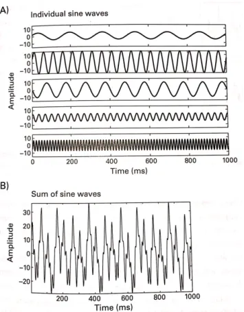
When combining different sine waves with different frequencies and different amplitudes, it is possible to create a complex electrical waveform as shown
in Figure 2-3. This is the case with the brain wave activity. Brain wave activity is composed of many single electrical sine waveforms as presented in Figure 2-4. It is possible to separate each component of the brain wave activity with a method called Fast Fourier Transform (FFT) as presented in Figure 2-5, which will be explained in more detail in chapter 5.
Figure 2-3 Visual representation of different sine waves a) Presents many different sine waves, each with different magnitude and frequency. b) All the sine waves from a) can be sum resulting in a new complex signal (sum of sine waves) as presented in b) (Source: Cohen, 2014) Reprinted from “Analysing Neural Time Series Data: Theory and Practice” by Mike X. Cohen. Copyright © 2014 by Mike X. Cohen. Used by permission of The MIT Press, Cambridge, MA, USA.
When the brain wave activity signal is separated in its different components (using FFT), it is seen that the behaviour of the brain wave activity changes depending if an individual is awake or asleep (Cohen, 2014; Vuckovic et al., 2002).
Figure 2-4 Example of brain wave activity recorded from a human participant. Each line represents an electrode, which measures the brain wave activity (in microvolts), in different locations in the scalp of an individual (Source: Cohen, 2014) Reprinted from “Analyzing Neural Time Series Data: Theory and Practice” by Mike X. Cohen. Copyright © 2014 by Mike X. Cohen. Used by permission of The MIT Press, Cambridge, MA, USA.
When an individual is awake, signals with frequencies around 13 to 20 Hertz (Hz) have a high amplitude compared to signals with frequencies around 4 to 13 Hz (Filtness et al., 2012; Zhao et al., 2012; Lowden et al., 2009; Jap et al., 2009, Vuckovic et al., 2002). When an individual’s sleepiness is increasing, signals with frequencies around 13 to 20 Hz decrease in magnitude and signals with frequencies around 4 to 13 Hz have an increase in magnitude, specifically 8 to 13 Hz are the frequencies with the highest increase. When an individual is asleep, it has been found that frequencies around 30 Hz and above have an increase in amplitude (Vuckovic et al., 2002). For analysis purposes, many researchers have grouped and labelled the frequency ranges of the brain wave activity. There are four main frequency bands; the frequency interval of 4 to 8 Hz is called theta band, from 8 to 13 Hz is called alpha band, from 13 to 30 Hz is called beta band and frequencies above 30 Hz are categorise in the gamma band (Filtness et al., 2012; Zhao et al., 2012; Lowden et al., 2009; Jap et al., 2009, Vuckovic et al., 2002).
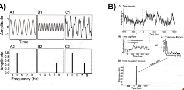
Figure 2-5 Effect of FFT in different sine waves a) Sine wave A1 (with amplitude 1 and frequency of 3 Hertz) and sine wave B1 (with amplitude 0.5 and frequency of 8 Hz) are combined to create signal C1. When FFT is performed in each of these sine waves, the result is decomposition of the frequencies belonging in each signal (as the sine waves A1 and B1 are just composed of a single sine wave with unique frequency the plot A2, B2 just present activity in one frequency. On the other hand, C2 presents activity in two frequency, as C1 is composed of two sine waves with different frequencies). b) An EEG (brain wave activity) signal (Figure B-A) is a composition of many sine waves with different frequencies; therefore, FFT analysis can be performed. In this case, a segment of the EEG data (Figure B-B) was analysed and the result can be plotted in the frequency domain (Figure B-C) or in the time-frequency domain (Figure B-D) (Source: Cohen, 2014) Reprinted from “Analysing Neural Time Series Data: Theory and Practice” by Mike X. Cohen. Copyright © 2014 by Mike X. Cohen. Used by permission of The MIT Press, Cambridge, MA, USA.
Using brain wave recording techniques to determine changes in different frequency bands, researchers have been able to determine and differentiate the awake and sleepy states in an individual, as presented in Figure 2-6. Within the sleep state, it has been possible to determine four different sleep levels (stage N1 to N3 and REM), as shown in Figure 2-6. Unfortunately for the awake state, is not easily classified.
Figure 2-6 Brain wave activity during awake and sleep stages. Sleep stages are categorised in 4 stages (N1, N2, N3 and REM) whilst awake is more difficult to classified in many stages (Source: Shi et al, 2017) Reprinted from “A comparison study on stages of sleep: Quantifying multiscale complexity using higher moments on coarse-graining” by Shi et al. Copyright © 2017 by Shi et al. Used by permission of Elsevier, Amsterdam, NL.
Once the effects of sleep in an individual and the different stages in awake and sleep have been presented, it is important to define the difference between the terms that used to describe awake and sleepy state in a driving scenario. In the following section, the different terms related to awake and sleep are explained in order to have a common understanding of the concepts that are referred to in later chapters of this thesis.
2.3.1 Alertness, drowsiness and sleepiness
In many research papers the terms drowsiness, sleepiness, and fatigue are used interchangeably to refer to a state where a person has the inability to stay awake (Filtness et al., 2012; Reyner et al., 2012; Wu & Chen, 2008; Yang et al., 2010; Zhao et al., 2012; Lowden et al., 2009; Jap et al., 2009, Vuckovic et al., 2002). In order to determine the effects of a driver falling asleep and waking up while driving, it is necessary to have a clear definition of sleepiness and its difference with other ‘awake’ and ‘sleepy’ stages such as alert, fatigue and drowsiness. For the purpose of this research, a common definition for these terms was determined using existing
definitions in literature.
2.3.1.1 Alertness (alert wakefulness)
This is the state of being awake and is commonly characterized by eye blink duration of 0.3 to 0.4 seconds and inter-eye blink of 6 to 8 seconds (Yeo et al., 2009; Hart, 1992; Doughty, 2002). During this state, beta activity in the brain is dominant (Hart, 1992).
2.3.1.2 Drowsiness (quiet wakefulness)
The stage prior falling asleep is called drowsiness (Johns, 2000). This state can be recognized by difficulty in maintaining visual focus attention, limitation of the higher cognitive functions, and limitations in the visual perception (Lamond & Dawson, 1999; Thomas et al., 1998). This level is also characterized by the appearance of microsleeps (Broughton & Hasan, 1995; Tanaka, Hayashi, & Hori, 1996) as well as increase in the alpha and theta activity in the brain and a decrease in the beta activity in the brain (Jap et al., 2009; Lal & Craig, 2001a,b; Stern & Engel, 2005; Yeo et al., 2009; Zhao et al., 2012; Akerstedt & Gillberg, 1990; Campagne, Pebayle & Muzet, 2004; Jap et al., 2009; Kecklund & Akerstedt, 1993; Lowden et al., 2009). The concept of microsleeps and alpha, theta and beta activity in the brain is explained further in section 2.5.
Drowsiness can also be distinguished by some physiological factors: eye blink duration of more than 0.5 seconds (Yeo et al., 2009), head nodding (Hartley et al., 2000; Haworth & Vulcan, 1991; Kaplan et al., 2007; Lal & Craig, 2002), increase in head movement (Berg & Landstrom, 2006) and yawning (Gu et al., 2002; Kaplan et al., 2007).
During drowsiness state, research found differences in driving performance such as an increase in lateral position variability as well as higher steering movements (Liu et al., 2009; Arnedt et al., 2001; De Valck & Cluydts, 2001; Ingre et al., 2006). Thiffault and Bergeron (2003) found that when drivers are in a drowsiness state, they make larger steering wheel movements (6-10 degrees) and fewer small steering wheel movements (1 – 5 degrees).
2.3.1.3 Fatigue
There is no agreed consensus in the literature on this term. For Brown (1994), fatigue is a state where a person would experience an unwillingness to continue a particular task. On the other hand, Bartlett (1953) stated that fatigue is a process that can be determined by changes in the performance of an activity in time. This term has been associated to sleepiness, as both terms are related to a reduction in attention and cognitive abilities.
2.3.1.4 Sleepiness
According to Johns (1998) and Curcio, Casagrande & Bertini (2001) sleepiness refers to the transition for someone to go from the stage of being awake to being in a drowsy or sleep stage at a particular time. Throughout this thesis, sleepiness is used as the measurement of sleep in the driver. Sleepiness can be affected by different factors:
1. Arousal level of the task being performed (Curcio et al., 2001). Monotonous1 roads are one of the main examples of low arousal tasks that affect the increase of sleepiness (Zhao & Rong, 2013). It has been found that driving on monotonous roads can lead to larger steering movements (overcorrections) compared to non-monotonous road (Thiffault & Bergeron, 2003). May & Baldwin (2009) defined this concept as task related sleepiness.
2. The length of time a person has been awake (Johns, 2000). This is mainly related to sleep deprivation and it is defined as a sleep related factor (May & Baldwin, 2009). After sleep deprivation, drivers have greater lane position variability, drive closer to the lane, have a higher standard deviation of their speed and have more unwanted lane crossings (Lenne et al., 1998; Philip et al., 2005). It has also been found that reaction time performance decreases with sleep deprivation (Graw et al., 2004; Philip et al., 2005).
3. The circadian rhythm (Borbély, Achermann, Trachsel, & Tobler, 1989). The circadian rhythm refers to a 24-hour biological cycle of every being that determines the patterns of sleeping and feeding (Vitaterna,
1“According to MacBain (1970) a situation is said to be monotonous when then stimuli remain unchanged or change in a predictable manner, resulting in sensory stimulation that is constant or highly repetitive”
Takahashi, & Turek, 2001). This means that during a 24-hour period, there are moments when human beings are more prone to fall asleep, usually being maximal at 3 a.m. to 4 a.m. (Borbély et al., 1989; Monk, 2005; Dinges, 1989; Tune, 1969). Pack et al. (1995) found that sleep crashes occurred more often between 2am and 6am and between 2pm and 4pm, this last one as a consequence to an increase in sleepiness due to a circadian rhythm period called ‘Afternoon dip’ (Monk, 2005).
2.4
Variables used to predict sleepiness
One important step to prevent accidents of people falling asleep while driving is to detect sleepiness before an accident occurs. This issue arises because there is not yet a consensus in literature regarding if drivers are unable to determine or predict that they will fall asleep with enough accuracy. According to Di Stasi et al. (2012), drivers are not aware and/or deny impairment of their driving skills due to fatigue. It is also very difficult to assess sleepiness in driving condition as drivers try to resist sleep while struggling to maintain alertness (Yeo et al., 2007; Eoh et al.; Monk 2005; Thiffault & Bergeron, 2003; Liang et al., 2005; Moller et al., 2006). On the other hand, Williamson et al. (2014) found that drivers were well aware of changes in the level of sleepiness. Further investigation in this topic needs to be done to reach a consensus regarding the subjective assessment of drivers’ own levels of sleepiness.
2.4.1 PERCLOS
One of the most common indicators used to predict sleepiness is PERCLOS (PERcentage of eye CLOSure), which uses the percentage of time the pupil is 80% covered by the eyelid within a 1 to 3 minutes (Lal & Craig, 2001a,b; Hayami et al., 2002; May & Baldwin, 2009, Wierwille et al., 1996, Dinges & Grace, 1998). PERCLOS is considered one of the most accurate ways to predict sleepiness (Bergasa et al., 2006; Dinges et al., 1998; Mallis, 1999) and it is presently used commercially (Lexus-Europe, 2012; LumeWay, 2014).
The problem with PERCLOS is that environmental factors such as changes in the lighting in the road, headlight from other cars and air temperature might change
the behaviour of the eye blinks, as well creating problems for the device to correctly determine the eye closure (Horne & Reyner, 1996).
2.4.2 Driving behaviour
Another way to determine sleepiness is by analysing the driving behaviour (Wakita et al., 2006; Takei & Furukawa, 2005; McCall et al., 2005). As stated before, an increase in standard deviation and steering wheel movement is related to an increase in sleepiness (Arnedt et al., 2001; Liu et al., 2009; De Valck & Cluydts, 2001; Ingre et al., 2006). This method to determine sleepiness is also used commercially by Bosch and Daimler who have created a device that depending on the lateral deviation of the car, the sleepiness of the driver can be determined (Bosch, 2012).
Unfortunately, driving behaviour changes from driver to driver, therefore it is difficult to assess changes in sleepiness in relation to driving behaviour (Liu et al., 2009). As such, driving behaviour has often been used in combination with other physiological measures to determine sleepiness in a more accurate way (Risser et al., 2000; Lal & Craig, 2002). As discussed previously, sleepiness affects the physiology and behaviour of an individual, so it is possible to use those physiological and behavioural changes as an indicator of sleepiness.
2.4.3 Physiological variables
The analysis of physiological variables such as head nodding, heart rate and body movement have been found to be closely related with sleepiness (Hartley et al., 2000; Haworth & Vulcan, 1991; Zilberg et al., 2007, 2009; Apparies et al., 1998; Li et al., 2004; Hartley et al., 1994). The relation between some of these measures with sleepiness is so strong that it has led to the development of devices to predict sleepiness. For example, NapZapper (2008-2016) created a commercial device using head nodding as a method to determine sleepiness.
The downside of using physiological variables is that the frequency and length of appearances of these physiological variables changes between individuals (Lal & Craig, 2002; van den Berg & Landstrom, 2006). Similar to the case of using
driving behaviour to predict sleepiness, the individuality of driver’s physiological behaviour makes it difficult to predict sleepiness with high accuracy.
2.4.4 EEG as the ground truth
Electroencephalogram (EEG) is one of the most reliable and precise indicators of sleepiness (Artaud et al., 1994; Lal et al., 2003; Jap et al., 2009). As such, it often serves as the gold standard, or a “ground truth” measure of sleepiness. It has been found that most of the drivers’ EEG measurements have a common behaviour, i.e. EEG is less affected by individuality of the participants (Jap et al., 2009; Lal & Craig, 2001a,b; Stern & Engel, 2005; Yeo et al., 2009; Zhao et al., 2012; Akerstedt & Gillberg, 1990; Campagne, Pebayle & Muzet, 2004; Jap et al., 2009; Kecklund & Akerstedt, 1993; Lowden et al., 2009). EEG has not been used commercially due to the difficulty to set up an EEG system in a real car (space is limited and the noise recorded in real driving is very high; Lal et al., 2003).
2.5
Brain wave and EEG as predictor of sleepiness
As mentioned before, brain wave activity has been used to determine awake and sleepy states. Brain wave activity can be recorded with different non-intrusive methods depending on the purpose and design of the research. The most common ways to record brain wave activity is using electroencephalogram (EEG), functional magnetic resonance image (fMRI) and Functional near-infrared spectroscopy (fNIR). In the following section, advantages and disadvantages of these techniques are discussed.
fMRI is a technique that uses a standard magnetic resonance scanner to create images of the brain (Lindquist & Wager, 2014). fMRI has a great spatial resolution, i.e. it is possible to determine the location in the brain where the electrical activity occurred (Lindquist & Wager, 2014; Cohen, 2014). Unfortunately, the temporal resolution of the fMRI is poor compared to other techniques, i.e. there is latency between the time the electrical activity occurs and the time is recorded by the fMRI (Lindquist & Wager, 2014). Finally, it is difficult to use fMRI in a driving experiment due to the size of most fMRI and the constraint position of the participants while using fMRI. In terms of the environment, there is also the
constraint of objects around the fMRI, e.g. metallic objects, which could harm the subjects and create interference with the fMRI (European Commission, 2013).
EEG is a technique of positioning a net with electrodes (the number of electrodes can differ from 32 to more than 200) on the head of an individual (Cohen, 2014), as shown in Figure 2-7. The electrical activity in the brain travels across the neurons until it reaches the scalp where the EEG records it. Compared to fMRI, EEG has very good temporal resolution but poor spatial resolution.
Figure 2-7 EEG net cap with 129 electrodes (used to record brain wave activity) held together with a transparent rubber net. Electrodes are soaked in potassium chloride electrolyte to allow better conductivity. The impedance, which measures the conductivity between the scalp and the electrode, was kept under 100 ohms.
fNIR is a technique that uses infrared sensors to detect changes in the concentration of oxygenated and deoxygenated haemoglobin in the blood, which is related to cerebral activity (León-Carrión & León-Domínguez, 2012). Although this technique is easier than positioning multiple electrodes, as with the EEG, the temporal resolution of the fNIR is worse than the temporal resolution of the EEG. EEG has the best characteristics to record brain wave activity in situations where temporal resolution, is very important, such as driving.
Brain wave activity, analysed through EEG, has been found to be a strong predictor of sleepiness while driving (Lal & Craig, 2002; Eoh, Chung & Kim, 2005;
Jap et al., 2009). Specifically, the brain wave activity related to sleeping while driving consists of four main frequency bands. Delta 𝜹 (0-4 Hz) and theta 𝜽 (4-8 Hz) are known as slow waves activity, and alpha 𝜶 (8-13 Hz) and beta 𝜷 (13-20 Hz) are known as fast wave activities (Lal & Craig, 2002; Eoh, Chung & Kim, 2005; Jap et al., 2009; Fisch, 2000; Hallvig et al., 2013; Filtness et al., 2012). Although these frequency ranges are commonly used, the frequency interval for each band may differ between different researchers.
Figure 2-8 Depending on the activity, EEG data (brain wave activity) can be classified in different frequency bands. After performing an FFT in raw EEG data, frequencies from 0-4 Hz belong to the delta band, 4-8 Hz to the theta band, 8-13 to the alpha band and 13-30 to the beta band. Different levels of sleepiness can be determined by analysing the power of each frequency band. (Source: Mohamed et al., 2017) Reprinted from “Towards automated quality assessment measure for EEG signals” by Mohamed et al. Copyright © 2017 by Mohamed et al. Used by permission of Elsevier.
A decrease in beta activity, especially in the temporal and frontal region of the scalp, is related to the increase of sleepiness while driving (Jap et al., 2009; Lal & Craig, 2001a,b; Stern & Engel, 2005; Yeo et al., 2009; Zhao et al., 2012). In addition, an increase in alpha (especially in the occipital region; Yeo et al., 2009) and theta activity (particularly in the frontal, temporal and occipital regions; Yeo et al., 2009) is closely related to an increase in sleepiness of the driver (Akerstedt & Gillberg, 1990; Campagne, Pebayle & Muzet, 2004; Jap et al., 2009; Kecklund & Akerstedt, 1993; Zhao et al., 2012; Lowden et al., 2009) although Eoh, Chung & Kim (2005) found
Raw EEG data
Delta Theta Alpha Beta Am p lit u d e time