Model Uncertainty and Endogenous Volatility
William A. Branch
University of California, Irvine
George W. Evans
University of Oregon
October 18, 2005
Abstract
This paper identifies two channels through which the economy can generate endogenous inflation and output volatility, an empirical regularity, by intro-ducing model uncertainty into a Lucas-type monetary model. The equilibrium path of inflation depends on agents’ expectations and a vector of exogenous random variables. Following Branch and Evans (2004) agents are assumed to underparameterize their forecasting models. A Misspecification Equilibrium arises when beliefs are optimal given the misspecification and predictor pro-portions based on relative forecast performance. We show that there may exist multiple Misspecification Equilibria, a subset of which are stable under least squares learning and dynamic predictor selection. The dual channels of least squares parameter updating and dynamic predictor selection combine to gen-erate regime switching and endogenous volatility.
JEL Classifications: C53; C62; D83; D84; E40
Key Words: Lucas model, model uncertainty, adaptive learning, rational expectations, volatility.
1
Introduction
Time-varying volatility in inflation and GDP growth is an empirical regularity of the U.S. economy. This observation is often described in the applied literature as a regime shift during the 1980’s which resulted in a simultaneous decline in inflation and output volatility. The ‘Great Moderation’, econometrically identified by Stock and Watson (2003) and McConnell and Quiros (2000), among others, is often associated with a change in the stance of monetary policy (e.g. Branch, Carlson, Evans and McGough (2004)).
However, recent studies by Cogley and Sargent (2005) and Sims and Zha (2005) present evidence that drifting and regime switching inflation and output volatility
is a characteristic of the post-war period. Since the Great Moderation consists of a one-time simultaneous decline in volatility, and its timing coexists with changes in Federal Reserve policy, it seems natural to seek policy explanations of this particular event. Persistently evolving inflation volatility may not always go hand in hand with changes in Federal Reserve policy. In this paper, we demonstrate that drift and regime switching in volatility may arise endogenously through model uncertainty.
Private sector expectations of future economic variables play a key role in most monetary models (e.g. Woodford (2003)). In these self-referential models, agents’ beliefs feed back positively onto the underlying stochastic process. Yet, there is no consensus among economists on how agents actually form their expectations. While Rational Expectations provides a natural benchmark, there is a rapidly expanding lit-erature, e.g. Marcet and Sargent (1989), Brock and Hommes (1997), Sargent (1999), Evans and Honkapohja (2001), and Marcet and Nicolini (2003) that replaces rational expectations with statistical learning rules. This alternative approach, it is argued, is a reasonable description of agents’ actual forecasting acumen because it assumes behavior consistent with econometric practice.
Branch and Evans (2004), though, note that with computational costs and de-gree of freedom limitations, econometricians often underparameterize their forecast-ing models. It has long been recognized that Vector Autoregressive (VAR) models have degrees of freedom limitations. Recent work by Chari, Kehoe, and McGrattan (2005) argue that these limitations present obstacles to VAR researchers who try to uncover a model’s stochastic structure from observable time-series variables. The ap-proach in this, and our earlier, paper is to model agents as VAR econometricians who behave optimally given the restrictions imposed on them by the data. The previous paper, developed in the context of the cobweb model, derived heterogeneity as an equilibrium outcome when agents choose the dimension in which to underparame-terize. The current paper revisits that approach, instead framing the analysis in a Lucas-type monetary model along the lines of Evans and Ramey (2004).
We confront agents with a list of underparameterized predictor functions. The economic model is self-referential in the sense that agents’ expectations, a function of their underparameterization choice, depends on the underlying stochastic process which, in turn, depends on these beliefs. A Misspecification Equilibrium (ME) is a fixed point of this self-reinforcing process. Model uncertainty arises in the sense that agents pick the best-performing statistical model. In our framework, what constitutes the best performing model depends not only on the regressors of the model, but also on the forecasting model choices of other agents. Of course, there are other ways to treat model uncertainty, for instance uncertainty about parameters (Hansen and Sargent (2005)) or about the form of the monetary policy rule. However, we believe that econometric model uncertainty is an important component of agent behavior, and this paper studies its implications.
There are two primary results in the current paper: first, when there are multiple underparameterized models from which agents must choose one, there may exist multiple stable equilibria each with distinct stochastic properties; second, when agents must adaptively learn the forecast accuracy of these models the economy will generate endogenous variation in inflation and output volatility.
This paper specifies a simple monetary model in which aggregate supply and ag-gregate demand depend on a vector of autoregressive exogenous disturbances and supply additionally depends on unanticipated price level changes. Motivated by the idea that cognitive and computing time constraints and degrees of freedom limitations lead agents to adopt parsimonious models, we impose that agents only incorporate a subset of these variables into their forecasting model. Following Branch and Evans (2004) we require that these expectations are optimal linear projections given the underparameterization restriction and that agents only choose best performing sta-tistical models. Despite the bounded rationality assumption, this remains in the spirit of Muth (1961) in the sense that for each statistical model the parameters are chosen optimally. An equilibrium in beliefs and the stochastic process is a Mis-specification Equilibrium. An ME extends the notion of a Restricted Perceptions
Equilibrium, which arise in the models of Evans, Honkapohja, and Sargent (1993),
Evans and Honkapohja (2001), and Sargent (1999), to settings in which agents must choose their models. We show that in the Lucas model there exist multiple ME and, moreover, the ME with homogeneous expectations are stable under least squares learning.
One implication of our theoretical model is that in a real-time dynamic version of the model agents must simultaneously estimate the parameters of their forecasting model and choose the best model based on past experience. We show that when agents use least squares to estimate the parameters of their statistical model, and base forecast performance on average mean-square forecast error of the competing models, different Misspecification Equilibria, in each of which agents coordinate on one forecasting model, can be stable.
Most interestingly, “constant gain” dynamics lead to new and distinct results. Constant gain least squares algorithms place a greater (time-invariant) weight on more recent observations. Constant gain (or “perpetual”) learning, has been studied, for example, by Sargent (1999), Cho, Williams, and Sargent (2002) and Orphanides and Williams (2005a), who argue for the plausibility of this form of learning dynamics as a way in which agents would allow for possible structural change. In this paper we extend this idea in an important way: learning jointly about model parameters and model fitness. Model uncertainty arises via constant gain learning and dynamic predictor selection.
Extending constant gain learning to incorporate dynamic predictor selection, we identify two channels through which inflation and output volatility may evolve over
time. The first channel is from the parameter drift induced by constant gain updating of the forecasting model parameters. Under constant gain learning, the parameters vary around their mean values, even if the economy remains at a single equilibrium. In addition, regime switching in inflation and output volatility can arise when the economy switches endogenously between high and low volatility equilibria. Thus, the second channel is through dynamic predictor selection when agents react more strongly to recent forecast errors than distant ones when assessing the fitness of a forecasting model. Through numerical simulations, we show that, when there is dynamic predictor selection and parameter drift, the dynamic paths of inflation and output are consistent with the empirical regularities identified by Cogley and Sargent (2005) and Sims and Zha (2005).
Our paper builds upon Brock and Hommes (1997, 1998), who study dynamic predictor selection in deterministic models using a similar reduced form to the model used here.1 Branch and Evans (2004) extend Brock and Hommes to a stochastic
environment in which, in equilibrium, both the choice of forecasting model and the parameters of each predictor are determined simultaneously. In that paper, we show that an equilibrium can arise in which agents are distributed heterogeneously across forecasting models. The contribution of the current paper is to demonstrate the possibility of multiple equilibria in an economic model with positive expectational feedback, and to show that dual learning in parameters and predictor selection can therefore generate the type of dynamics arguably present in macroeconomic time series.
This paper proceeds as follows. Section 2 presents evidence of time-varying volatil-ity in the U.S. economy. Section 3 presents the Lucas model with model uncertainty. Sections 4 and 5 consider the model under real-time learning. Section 6 concludes.
2
Inflation and Output Volatility in the U.S.
2.1
An Empirical Overview
In the applied literature there is widespread consensus that during the 1980’s there was a decline in economic volatility. An array of econometric techniques to identify the regime shift have been employed by Bernanke and Mihov (1998), Kim and Nelson (1999), Kim, Nelson, and Piger (2004), McConnell and Quiros (2000), Sensier and van Dijk (2004), and Stock and Watson (2003). Recently, though, Cogley and Sargent (2005) and Sims and Zha (2005) have identified repeated regime shifting economic volatility in U.S. inflation and GDP growth. While Cogley-Sargent and Sims-Zha are
1Evans and Ramey (1992) examined dynamic predictor selection when agents choose between
interested in characterizing changing monetary policy over the period they make a striking finding: during the post-war period there is persistent stochastic volatility in the economy.
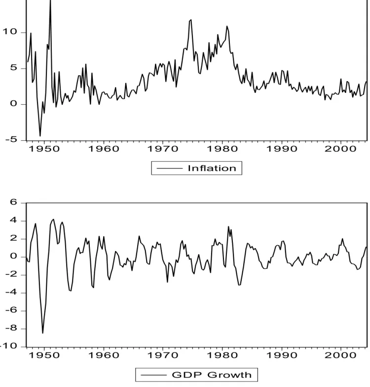
Conventional macroeconomic models, however, are unable to generate persistent stochastic volatility without directly assuming either exogenous disturbances follow-ing a Markov chain or exogenous changes in policy. In this paper, we present a model capable of generating such volatility endogenously via an adaptive learning and dynamic predictor selection process in a setting where agents may choose be-tween competing underparameterized forecasting models. First, though, this section presents an informal accounting of the nature of stochastic volatility in the economy. We present a series of plots, each some variant on quarterly inflation computed from the GDP deflator and quarterly GDP, which suggests the presence of stochastic volatility rigorously documented by Cogley and Sargent (2005) and Sims and Zha (2005). Our purpose here is motivation and overview; we refer the reader to these other papers for formal econometric analysis. We detrend the log of real GDP using the Hodrick-Prescott filter since in the Lucas model below output is expressed as a log deviation from its trend value. Figure 1 plots inflation and (detrended) GDP for the period 1947:1-2002:2.
INSERT FIGURE 1 HERE
Inspection of Figure 1 demonstrates the ‘Great Moderation’ emphasized by Mc-Connell and Quiros (2000) and Stock and Watson (2003). About 1984 there was a simultaneous decline in the volatility of inflation and GDP. This empirical feature has generated considerable recent research into monetary policy’s role in bringing about the observed economic stability.2 Broader inspection of the data, though, suggests
that this was not the only simultaneous change in economic volatility. GDP appears to be slowly stabilizing throughout the sample with the exception of a period in the late 1970’s. Inflation, on the other hand, seems to persistently change between high and low volatility states.
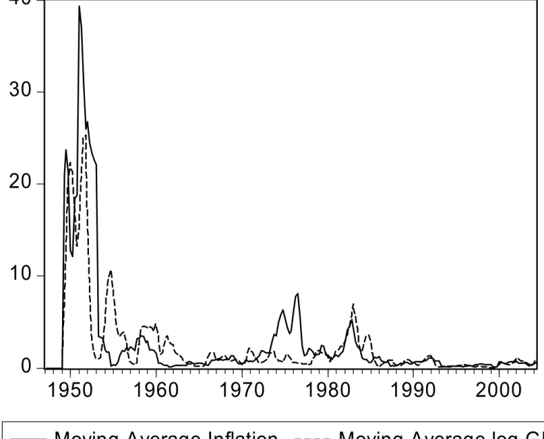
To further inspect the time-varying volatility of inflation and GDP suggested by Figure 1, Figure 2 calculates moving average estimates of the unconditional variance of inflation and GDP using a rolling window of 8 quarters. These calculations provide a rough estimate of how actual volatility changed over time. Figure 2 demonstrates, as Figure 1 suggested, that the volatility of GDP and inflation varies over time. In particular, each series appears to move in tandem and alternate between high and low variance regimes. Sims and Zha (2005) find that 9 separate regimes fit the data best. This plot resembles the posterior mean estimates for the standard errors of the VAR innovations in Cogley and Sargent (2005) over the period 1960-2000.
INSERT FIGURE 2 HERE
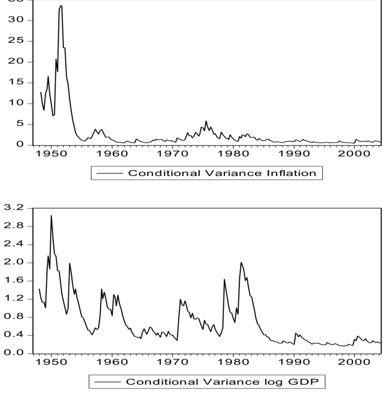
Owyang (2001) presents evidence that inflation follows an ARCH process. Figure 3 plots the conditional variances from an ARCH specification for inflation and GDP to demonstrate the robustness of the finding that there is persistent stochastic volatility in both inflation and GDP. To compute the conditional variances in Figure 3 we estimated a GARCH(1,1) for an AR(4) model of inflation and GDP. This follows exactly Owyang (2001) except that we also estimate a GARCH model for the volatility of GDP. Figure 3 then plots the conditional variances from the GARCH models.
INSERT FIGURE 3 HERE
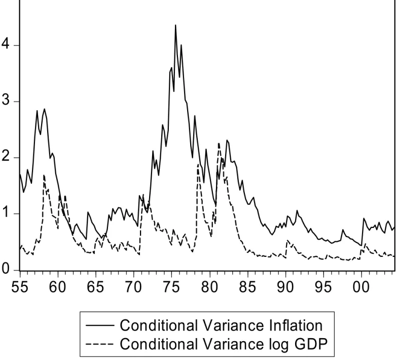
Figure 3 demonstrates that persistent and changing volatility is a hallmark of the data. In particular, apparent regime switching volatility is seen in both data series, and not just at the time of the Great Moderation, though the period since 1985 does emerge as one of unusual stability. Figure 4 plots the same conditional variance series as Figure 3, except that it focuses on the period 1955:1-2002:4. Figure 4 illustrates the presence of persistent stochastic volatility even when the high volatility period in the early 1950s is excluded.
INSERT FIGURE 4 HERE
2.2
Discussion
Despite the attention given the Great Moderation, there seems to be little emphasis in the theoretical literature on accounting for the persistent stochastic volatility of the economy. Sims and Zha (2005) seek evidence in a change in the stance of mone-tary policy repeatedly across time. Sargent (1999) presents a theory of the rise and fall in inflation that is the result of drifting beliefs on the part of the government.3
Orphanides and Williams (2005a) account for the decline in volatility as a change in the stance of policy which pins down agents’ drifting beliefs.
In this paper, we develop another possible explanation that does not require policy changes. We present a model in which agents must choose between two alternative underparameterized models. We demonstrate the possibility of multiple coordinating equilibria with distinct stochastic properties across equilibria. We introduce model uncertainty by assuming that agents use constant gain least squares to estimate the parameters of their forecasting model. This introduces drifts into their beliefs as in
3Over a long stretch of time this would be expected to lead to periodic regime changes due to
Sargent (1999) and Orphanides and Williams (2005a). We also augment the model to allow agents to choose their forecasting model in real time based on a geometric weighted average of recent forecast performance. In this version of the model, agents switch persistently and endogenously between forecasting models. This induces the economy to switch between high and low inflation variance equilibria. Thus, we provide two possible sources of stochastic volatility: drifting beliefs and endogenous predictor selection.
It should be emphasized that we do not in any way discount the role for other explanations of persistent stochastic volatility, such as major shifts in macroeconomic policy. However, we do feel that the channels identified here, developed in the context of a very simple and otherwise well-behaved macroeconomic model, appear to be sufficiently powerful to merit serious empirical investigation in future research.
3
Model
This section extends the Branch and Evans (2004) cobweb model with misspecification to a Lucas-type monetary model. In Branch and Evans (2004) firms choose planned output based on a misspecified forecasting model of the market price. Misspecification is modeled by confronting agents with a list of underparameterized models. Agents do, however, forecast optimally in the sense that they only choose the best performing statistical model. That paper establishes that, under appropriate joint conditions on the self-referential feature of the model and the exogenous disturbances, agents will necessarily be distributed heterogeneously across misspecified models.
Here we establish the existence of misspecification equilibria in a closely related Lucas-type monetary model. Later sections will address the dynamics of learning and predictor selection. Although the reduced form of the Lucas model is similar to the cobweb model, the slopes of the two models have opposite signs. The negative feedback of the cobweb model plays a central role in the existence of Intrinsic Hetero-geneity. In the Lucas model the feedback from expectations is positive. The reinforc-ing aspect of expectations induces coordination by agents and raises the possibility of multiple equilibria. A striking feature of our results is that underparameteriza-tion makes multiple equilibria possible in a well-behaved model that has a unique equilibrium under fully rational expectations.
3.1
Set-up
Following Evans and Ramey (1992, 2003) we assume the economy is represented by equations for aggregate supply (AS) and aggregate demand (AD):
AS :qt = φ(pt−pet) +β1zt
AD:qt = mt−pt+β2zt+wt
where pt is the log of the price level, pet is the log of expected price formed in t−1,
mt is the log of the money supply, qt is the deviation of the log of real GDP from
trend, and ηt is an iid zero-mean shock. Assume that the money supply follows,
mt = pt−1+δ0zt+ut
zt = Azt−1+εt
We assume for simplicity thatztis (2×1) andεtisiid zero-mean with positive definite
covariance matrix Σε. The vectorzt is also assumed to be a stationary process with
the eigenvalues of A inside the unit circle. The stochastic disturbance zt collects the
serially correlated disturbances that affect aggregate supply, aggregate demand, and the money supply. The matricesβ1, β2, δ determine which components of z affect the
respective reduced form relationships via (possible) zero components.
Denoting πt = pt−pt−1 we can write the law of motion for the economy in its
expectations-augmented Phillips curve form
πt= φ 1 +φπ e t + (δ+β2 −β1) 0 1 +φ zt+ 1 1 +φ(wt+ut) or πt=θπet +γ 0 zt+νt (1) whereθ= 1+φφ, γ0 = (δ+β2−β1)0 1+φ , νt= 1
1+φ(wt+ut). Note, in particular, that 0≤θ <1.
The cobweb model also takes the reduced form (1), but with θ < 0. This case is considered in Branch and Evans (2004).
Arational expectations equilibrium (REE) is a stationary sequence{πt}which is a
solution to (1) given πte=Et−1πt, whereEt is the conditional expectations operator.
It is well-known that (1) has a unique REE and that it is of the form
πt = (1−θ)−1γ0Azt−1+γ0εt+νt (2)
Output, in an REE, is white noise and does not display the time-series properties evident in the previous section. If instead agents only took one component of z into account when forecasting inflation then the reduced form weights on the components of zt will change. Such a deviation from the REE (2) is a key insight of our model.
3.2
Model Misspecification
This paper departs from the rational expectations hypothesis (RE) and imposes that agents are boundedly rational. One popular alternative to RE is to model agents as econometricians (e.g. Evans and Honkapohja (2001)). According to this litera-ture, agents have a correctly specified model whose parameters are estimated from a reasonable estimator. In many instances, these beliefs converge to RE. In prac-tice, however, econometricians often misspecify their models. Professional forecasters often restrict the number of variables and/or lags to conserve degrees of freedom. In-deed, Chari, Kehoe, and McGrattan (2005) argue that econometric misspecification is central to the debate over identified Impulse Response Functions. Following Evans and Honkapohja (2001), Evans and Ramey (2004), and Branch and Evans (2004), we argue that if agents are expected to behave like econometricians then they can also be expected to misspecify their models. We impose misspecification by forcing agents to underparameterize in at least one dimension. We follow Evans and Honkapohja (2001, Ch. 13), however, and impose that these underparameterized beliefs are opti-mal linear projections given the misspecification.
In this Section we begin by defining the restricted perceptions equilibrium, given the misspecified models available and the proportion of agents using each model. In Section 3.3 we allow the model to endogenously determine the proportions and define a Misspecification Equilibrium. Then, in Section 4 we study the real-time dynamics of the model, with optimal projections replaced by least squares estimates and model choices determined by dynamic predictor selection based on recent performance.
Beliefs are formed from models that take one of the following forms:
πte = b1z1,t−1 (3)
πte = b2z2,t−1. (4)
Because zt is a bivariate VAR(1) it is clear that (3)-(4) represents all possible
non-trivial underparameterized models. Informally, we view the true economic process as being driven by a high dimensional exogenous process. That agents underparameter-ize, or approximate their econometric models, is a reasonable description of actual forecasting behavior. The assumption that zt is bivariate VAR(1) is, of course, made
for analytical convenience. One can show the existence of Misspecification Equilibria, more generally, if zt is n×1 and follows a VAR(p). We impose that the parameters
b1, b2 are formed as optimal linear projections of πtonzi,t fori= 1,2. That is, beliefs
satisfy the orthogonality condition
Ezi,t−1 πt−bizi,t−1
= 0 (5)
This condition ensures that, in an equilibrium, agents’ beliefs are consistent with the actual process in the sense that their forecasting errors are undetectable within their
perceived model. When this occurs we say the model is at a Restricted Perceptions Equilibrium (RPE).4
Equilibria based on model misspecification that satisfy an orthogonality condition like (5) appear frequently in the literature. Rational expectations equilibria with limited information were studied in Sargent (1991) and Marcet and Sargent (1995), and Sargent (1999) examined the closely related concept of self-confirming equilibria. Consistent expectations equilibria, in which agents have linear beliefs consistent with a non-linear model, were developed in Hommes and Sorger (1998) and extended to stochastic models by Hommes, Sorger, and Wagener (2002) and Branch and McGough (2005). In Adam (2005a), one of the two possible model equilibria is an RPE. Evans and Ramey (2004) study optimal adaptive expectations in a Lucas-type model when the exogenous shock follows a complicated, unknown process. All of these approaches share the idea, exploited here, that agents are likely to misspecify their econometric model, but (in equilibrium) will do so optimally, given their misspecification.5
Of course, in the example we develop in this paper, with two underparameterized models, the misspecifications would be easily identified by an experienced econome-trician. To obtain tractable analytical results we develop our ideas using the simplest possible case, with a single endogenous variable of interest and a pair of exogenous variables following a VAR(1) process. Our analysis should be understood as a simpli-fication of a much more complex economy with many endogenous variables of interest, driven by multiple exogenous observables following high order processes. We submit that the central themes of this paper would emerge in a more realistic model in which positive feedback from expectations plays an important role.
Because agents may be distributed heterogeneously across predictors, actual mar-ket beliefs for the economy are a weighted average of the individual beliefs
πte=nb1z1,t−1+ (1−n)b2z2,t−1
wheren is the proportion of agents who use model 1.6 Inserting these beliefs into (1)
leads to
πt=θ nb1z1,t−1+ (1−n)b2z2,t−1
+γ0Azt−1+γ0εt+νt
Or, by combining similar terms,
πt=ξ1z1,t−1+ξ2z2,t−1+ηt (6)
4Adam (2005b) presents experimental evidence for approximate RPE in a bivariate macro model
of output and inflation.
5See also Guse (2005), who looks at “mixed expectations equilibria,” in which a given proportion
of agents may underparameterize the solution.
6We identify model 1 as the model with thez
where
ξ1 = γ1a11+γ2a21+θnb1,
ξ2 = γ1a12+γ2a22+θ(1−n)b2,
ηt =γ0εt+νt, and aij is the ijth element of A. It follows from (5) and (6) that the
optimal belief parameters are
b1 = ξ1+ξ2ρ
b2 = ξ2+ξ1ρ˜
whereρ=Ez1z2/Ez12 and ˜ρ=Ez1z2/Ez22.7 Note that theξparameters are functions
of b. Thus an RPE is a stationary process for πt which satisfies (6) with parameters
ξ1, ξ2 which solve 1−θn −θnρ −θ(1−n) ˜ρ 1−θ(1−n) ξ1 ξ2 =A0γ (7)
A unique RPE exists if and only if the matrix which premultiplies the parameter vector is invertible. We formalize this invertibility condition below:
Condition 4: 4 6= 0 for all n ∈[0,1] , where
4= 1−θ+θ2n(1−n)(1−ρρ˜)
Remark 1 Using the argument of Branch and Evans (2004) it can be shown that Condition 4 is satisfied for all θ <1.
3.3
Misspecification Equilibrium
A Misspecification Equilibrium (ME) is an RPE which jointly determines the fraction of agents using a given model. Below we formally define the equilibrium and present results on existence of ME.
We follow Brock and Hommes (1997) in assuming the map from predictor benefits to predictor choice is a multinomial logit (MNL) map.8 Brock and Hommes assume
that agents base their predictor decisions on recent realizations of a deterministic process. In an ME we instead assume agents base their decisions on the unconditional moments of the stochastic process. Later when we introduce learning and dynamic predictor selection the predictor choice is based on an average of past realizations.
7The existence of these unconditional moments are guaranteed by the stationarity ofz
t.
8The use of the multinomial logit in discrete decision making is discussed extensively in Manski
As in Evans and Ramey (1992) we assume agents seek to minimize their forecast MSE, i.e. we assume agents maximize
Eu=−E(πt−πet)
2
This assumption is reasonable in light of the linear R.E. literature and well-known results in least-squares prediction theory. If πet is conditional on full information then R.E. would minimize the expected mean-square error of one step-ahead forecasts. Thus, we preserve this structure when agents form optimal linear projections on a limited information set. The MNL approach leads to the following mapping, for each predictor i= 1,2, ni = exp{αEui} P2 j=1exp{αEuj} (8) Noting that P2 j=1nj = 1, (8) can be re-written n = 1 2 tanhhα 2 (Eu1−Eu2) i + 1≡Hα(Eu1−Eu2) where Hα :R→[0,1].
The parameter α, called the “intensity of choice,” measures the agents’ sensitiv-ity to changes in forecasting success. Brock and Hommes (1997) focus on the case of large but finite α. Branch and Evans (2004) note that a drawback to finite α is that agents are not fully optimizing. In our earlier paper, it was shown that in a stochastic framework where agents underparameterize their forecasting models, het-erogeneity may persist even as α → +∞. In the current paper, in the theoretical analysis we again emphasize the caseα →+∞, which enables us to provide a simple characterization of the possible ME. Then in Section 4, where we examine the system under real-time dynamics, we assume large, finite values of α.
One can verify that the MSEs of the predictors imply that Eu1 = ξ22 ρEz1z2−Ez22 −ση2 Eu2 = ξ12 ρEz˜ 1z2−Ez12) −ση2 Define the map F : [0,1]→R as
F(n) =Eu1−Eu2 =ξ12(1−ρρ˜) +ξ 2
2 ρ
2 −Q
where Q=Ez22/Ez12. If condition 4 is satisfied,F(·) is continuous and well-defined. Because condition 4 is satisfied for all θ ∈ [0,1), there exists a well-defined mapping Tα : [0,1]→[0,1] such that Tα =Hα◦F.
In a Misspecification Equilibrium the forecast parameters satisfy the orthogonality condition and the predictor proportions are determined by the MNL. In equilibrium, they are, therefore, both endogenously determined.
Proposition 2 A Misspecification Equilibrium exists.
This result follows since Tα : [0,1] → [0,1] is continuous and Brouwer’s theorem
ensures that a fixed point exists.9 By developing details of the map F we are able
to investigate further the set of ME.
Proposition 3 The function F(n) is monotonically increasing for all 0≤θ < 1.
The Appendix sketches the proofs to all propositions. Theoretical details that carry over from the cobweb model can be found in Branch and Evans (2004).
From the equation for expected utility it can be shown that F(1) ≷ 0 iff (1−ρρ˜)ξ12(1)≷(Q−ρ2)ξ22(1) F(0) ≷ 0 iff (1−ρρ˜)ξ12(0)≷(Q−ρ2)ξ22(0) where Q= Ez22
Ez2
1. Furthermore, from (7) we have (ξ1(1))2 (ξ2(1))2 = ((γ1a11+γ2a21) + (γ1a12+γ2a22)θρ) 2 (1−θ)2(γ 1a12+γ2a22)2 ≡B1 (ξ1(0))2 (ξ2(0)) = (γ1a11+γ2a21) 2(1−θ)2 ((γ1a11+γ2a21)θρ˜+γ1a12+γ2a22)2 ≡B0
Note that 0 < B0 < B1. Recall thatQ, ρ, and ˜ρ are determined by A and Σε. The
above results and Proposition 3 imply:
Lemma 4 There are three possible cases depending on A, θ, γ and Σ:
1. Condition PM: F(0) <0 and F(1) > 0. Condition PM is satisfied when (1− ρρ˜)B0+ρ2 < Q <(1−ρρ˜)B1+ρ2.
2. Condition P1: F(0) > 0 and F(1) > 0. Condition P1 arises when Q < (1− ρρ˜)B0+ρ2.
9Branch and Evans (2004) prove existence of a Misspecification Equilibrium for ann-dimensional
vectorztfollowing a stationary VAR(p) process, and an arbitrary list of misspecified models, provided
3. Condition P0: F(0) < 0 and F(1) < 0. Condition P0 arises when Q > (1− ρρ˜)B1+ρ2.
Remark: ρρ˜= 1 is ruled out by the positive definiteness of Σε.
Below we give numerical examples of when each condition may arise.
Under Condition PM, F(0) < 0 and F(1) > 0 implies that either model is prof-itable so long as all agents coordinate on that model; that is, there is no incentive for agents to deviate from homogeneity. When Condition P1 or P0 holds one model always dominates the other.
Lemma 4 allows for a characterization of the set of Misspecification Equilibria for large α. Let
Nα ={n∗|Tα(n∗) = n∗}
We now present our primary existence result for large α.
Proposition 5 Characterization of Misspecification Equilibria for large α:
1. Under Condition PM, as α → ∞, Nα → {0,n,ˆ 1} where nˆ1 is s.t. F(ˆn1) = 0.
2. Under Condition P0, as α → ∞, Nα → {0}.
3. Under Condition P1, as α → ∞, Nα → {1}.
The remainder of the paper is primarily concerned with Case 1 in which there are multiple equilibria. It should be briefly noted that an ME does not coincide with the unique REE in (2). For all n∗ ∈ Nα a comparison of (2) and the ME in
(6) and (7) (for a given n∗) shows that the ME has different relative weights on the exogenous variables.10 Interestingly, there may exist multiple ME even though
there is a unique REE. The ‘instability’ that results from misspecification is key for generating endogenous regime change in the Lucas model.
3.4
Further Intuition for Multiple Equilibria
The existence of multiple equilibria, and the resulting real-time learning and dynamic predictor selection dynamics, are key results. In this regard, greater intuition of
10Adam (2005a) considers a New Keynesian model where agents are restricted to univariate
fore-casting models. In his model, though, there exist equilibria which are REE. Guse (2005) also studies a model with multiple REE and where agents’ forecasting models are distributed across the repre-sentations consistent with each REE.
when multiple equilibria arises is useful. The existence of multiple equilibria, as demonstrated by Proposition 5, depends on the asymptotic properties of thezprocess, and on both the direct(γ0A) and indirect (θ) effect of z on inflation. This subsection presents the intuition on the relationship between the direct and indirect effects.
For ease of exposition, assume ρ = ˜ρ= 0. From Proposition 5 multiple ME arise when B0 < Q < B1, where B1 = (γ1a11+γ2a21)2 (1−θ)2(γ 1a12+γ2a22) 2 B0 = (γa11+γ2a21) 2 (1−θ)2 (γ1a12+γ2a22)2
Now suppose that θ = 0. Then B0 = B1 and there does not exist any Q, hence
any z, such that multiple equilibria exist. Instead suppose that θ→1. Then B0 →0
and B1 → ∞. In this instance, the entire range of uncorrelated, bivariate VAR(1)
will lead to multiple equilibria.
The condition PM places restrictions on the interaction between the direct and indirect effects of the model. When there is no feedback from expectations onto the state, then it is clear that agents will always choose the predictor with the highest direct effect. When the self-referential parameter is high, then the indirect effect magnifies the direct effect of the components of z. In these instances it is possible that coordination on a particular forecasting model will produce an indirect effect sufficiently stronger than the direct effect so that this predictor dominates in expected MSE. Significantly, the existence of multiple equilibria arises from the coordinating forces of positive feedback.
3.5
Numerical Examples
We turn now to a numerical illustration. Figure 5 gives the T-maps for various values of α. The upper part of the figure shows the T-maps corresponding to (starting from n= 0 and moving clockwise) α= 10, α= 20, α= 50, α= 1000. We set
A= .5 .001 .001 .3 γ0 = [.5, .75], Σε= .03 .001 .001 .15
INSERT FIGURE 5 HERE
The matrixA, Σε, andθhave been chosen so that Condition PM holds. Condition
PM holds under many other parameterizations as discussed above. We chose these parameters as they deliver quantitatively reasonable results in the section on real-time learning and dynamic predictor selection.
A key property of the model is that as α → ∞
Hα(x)→ 1 if x >0 0 if x <0 1/2 if x= 0 (9)
and this governs the behavior ofTα =Hα◦F. Since Hα is an increasing function and
F is monotonically increasing, it follows that Tα is increasing. Under Condition PM
it is clear that (9) implies existence of three fixed points forα sufficiently large. The figure illustrates this intuition.
This example makes it clear that multiple equilibria can exist in the Lucas-type monetary model. When agents underparameterize there is an incentive to coordinate on a particular forecasting model. Interestingly, though, there also exists an interior equilibrium. Below we show that this equilibrium is unstable under learning. The existence of multiple ME suggests there may be interesting learning phenomena in the model. We take up this issue in the section below.
The particular parameterization which leads to this figure produces the following asymptotic covariance matrix for zt:
Σz =
.04 .0013 .0013 .1648
Notice that the variance of z2 is approximately 4 times that of z1. The effect of this
can be seen in Figure 5 where the ‘basin of attraction’ for the n = 0 ME is larger than for then = 1 ME.A priori we would expect a real-time version of this economy to spend, on average, more time near n = 0 than n = 1. This logic will be key in Section 5 below.
It should be emphasized that in other contexts there may exist a unique interior ME. Branch and Evans (2004) illustrate this case by developing the framework in the context of the cobweb model. The existence of an ME with heterogeneity– what Branch and Evans (2004) call Intrinsic Heterogeneity– exists for precisely the opposite reasoning for multiple ME in the Lucas model. In the cobweb model there is negative feedback from expectations onto the state. Under certain conditions there is an incentive for agents to deviate from the consensus model. Thus, the equilibrium forces push agents away from homogeneity. In the Lucas model the equilibrium forces, as a
result of the positive feedback, push the economy towards homogeneity. These results illustrate the multiplicity of equilibrium phenomena that can arise depending on the self-referential features of a simple model.
4
Learning and Dynamic Predictor Selection
In this section we first address whether the Misspecification Equilibria are attainable under real-time econometric learning and dynamic predictor selection. We now re-place optimal linear projections with real-time estimates formed via recursive least squares (RLS). We also assume that agents choose their model each period based on an estimate of mean square error. In Section 5 we replace RLS with a constant gain updating rule of the form used, for example, in Evans and Honkapohja (1993), Sar-gent (1999) and Cho, Williams, and SarSar-gent (2002), and we also employ a constant gain version of the dynamic predictor selection introduced by Brock and Hommes (1997).
We replace the equilibrium stochastic process (6) with one that has time-varying beliefs and predictor proportions. Below we provide details on how the key relation-ships are altered. This section briefly discusses the stability of the equilibrium under recursive least squares. We model least squares learning as in Branch and Evans (2004). Agents have a RLS updating rule with which they form estimates of the be-lief parameters b1t, b2t. They also estimate the MSE of each predictor by constructing a moving average of past forecast errors with equal weight given to all time periods. Given estimates for the belief parameters and predictor fitness, agents choose their forecasting model according to the MNL map in real time.11
We now assume the equilibrium stochastic process is given by πt=ξ1(b1t−1, n1,t−1)z1,t−1+ξ2(b2t−1, n1,t−1)z2,t−1+ηt.
Agents use a recursive least squares updating rule, bjt =bjt−1+κtR−j,t1zj,t−1 πt−bjt−1zj,t−1 , j = 1,2. where Rj,t =Rj,t−1+κt zj,t2 −1−Rj,t−1 , j = 1,2.
We consider two possible cases for the gain sequence κt: under decreasing gain,
κt=t−1 so that κt→0; under constant gain, κt =κ∈(0,1).
11A point made in Branch and Evans (2004) is that stability of a steady-state depends on how
more recent forecast errors are weighted in the moving average calculation. In particular, as the most recent error is weighted more heavily then instability will result as in Brock and Hommes (1997, 1998).
We also assume agents recursively update mean-square forecast error according to
M SEj,t =M SEj,t−1+λt (πt−πj,te )2−M SEj,t−1
, j = 1,2.
We again consider two possible cases for the gain sequenceλt: under decreasing gain,
λt =t−1 so that λt →0; under constant gain, λt=λ∈(0,1).
We first look at the case of decreasing gain for both κt, λt. We then turn in the
next Section to our main emphasis of constant gain updating.
4.1
Stability under decreasing gain
In this subsection we study whether the sequence of estimates b1
t, b2t and predictor
proportions n1,t converge to a Misspecification Equilibrium.12 Our aim is to use
sim-ulations to ascertain which equilibria are stable under real-time learning and dynamic predictor selection. Establishing analytical convergence is beyond the scope of this paper.
We continue with the parameterization in the previous section which yielded mul-tiple ME. We set
A = .5 .001 .001 .3 ,Σε = .03 .001 .001 .15
and γ0 = [.5, .75]. We also set θ = .6 and α = 1000.13 We simulate the model for 5,000 time periods. The initial value of the VAR is equal to a realization of its white noise shock, i.e., z0 =ε0. The initial valuen1,0 is drawn from a uniform distribution
on [0,1] and bj,0, j = 1,2 is drawn from a uniform distribution on [0,2]. The initial
estimated variances are setR1,0 =R2,0 = 1.
Figure 6 illustrates the results of two representative simulations. The top panel plots the simulated proportionsntagainst time. Recall that for the chosen parameters
there exist three equilibria. The plot demonstrates that only the equilibria with homogeneous expectations are stable under learning and dynamic predictor selection. The dynamics quickly converge to either n= 0 or n= 1. The bottom panel plots the reduced form equilibrium parametersb1
t−1, b2t−1. In each panel there are two horizontal
lines which correspond to the parameter values in either the n = 0 or n = 1 ME. In the b1 panel the top horizontal line corresponds to the n = 1 equilibrium and in the b2 panel the top horizontal line is for the n = 0 equilibrium. As seen in the
top panel, these parameters converge to their ME values. Which equilibrium the dynamics converge to depends on the basins of attraction. As we emphasize in the
12Because the analysis is numerical we are being deliberately vague in what sense these sequences
converge.
13Similar results were obtained for other parameter settings. The speed of convergence is sensitive
next section, these basins are sensitive to the parameterization of the zt process.
Thus, we conclude that ME with n ∈ {0,1} are locally stable under learning and dynamic predictor selection.
INSERT FIGURE 6 HERE
The intuition for this stability is as follows. The multiple equilibria results from an incentive for agents to coordinate on a single model. These coordinating forces render the interior equilibrium, with heterogeneity, unstable under learning. Suppose the dynamics begin in a neighborhood of the interior equilibrium. Because the profit function is monotonically increasing, as more agents mass onto a particular model then more agents will also want to use that model. The dynamics are repelled from the neighborhood of the interior steady-state and towards one of the other ME. To which ME the dynamics converge depends on the basin of attraction in which the initial conditions lie.
This result is, again, distinct from the result in Branch and Evans (2004). In that paper, there is a unique Misspecification Equilibrium which is stable under learning. In the current paper we have multiple equilibria on the boundary of the unit interval that are locally stable under learning. This result leads to interesting dynamics when agents update with a constant gain learning algorithm.
5
Real-time Learning with Constant Gain
It has been suggested by Sargent (1999), among others, that agents concerned with structural change should use a constant gain version of RLS to generate parameter estimates. A constant gain algorithm involves a time-invariant gain which places a high relative weight on recent versus distant outcomes. If agents are concerned about structural change then a constant gain algorithm will better pick up a change in parameters. It has also been argued by Orphanides and Williams (2005a) that constant gain learning is more reasonable than RLS learning because the learning rule itself is stationary whereas it is time-dependent in RLS. Empirical support for constant gain learning is provided in Orphanides and Williams (2005b), Branch and Evans (2005), and Milani (2005).
In the Lucas model with misspecification we showed that there may exist multiple equilibria. Moreover, a subset of these equilibria are stable under learning with a decreasing gain algorithm such as RLS. In these equilibria there is an incentive for agents to coordinate on the same forecasting model. If a large enough proportion of agents suddenly switch forecasting models then the economy will switch from one
stable ME to another. Agents concerned with this possibility should use a constant gain algorithm instead of a decreasing gain to account for possible regime change.
There has been an explosion in research adopting constant gain learning rules. Examples include Bullard and Cho (2002), Cho and Kasa (2003), Cho, Williams, and Sargent (2002), Evans and Honkapohja (1993, 2001), Evans and Ramey (2004), Kasa (2004), Orphanides and Williams (2005a), Sargent (1999) and Williams (2004a,b). In many of these models constant gain learning can lead to abrupt changes or ‘escapes’ in the dynamics. For example, in models with multiple equilibria, such as Evans and Honkapohja (1993, 2001), occasional shocks can lead agents to believe the economy has shifted to a new equilibrium. The result of these beliefs is a self-confirming shift to the new equilibrium. Unlike sunspot equilibria, these shifts are driven entirely by agents’ recursive parameter estimates. In Sargent (1999), Cho and Kasa (2003), Cho, Williams, and Sargent (2002), Bullard and Cho (2002), and McGough (2004), occasional large shocks can lead to temporary deviations from the equilibrium that is uniquely stable under RLS.
The same logic underlying the use of constant gain RLS for parameter estimation carries over to the estimate of the relative fitness of the two forecast rules. Agents who are concerned about structural change, including shifts taking the form of occasional regime changes, would want to allow for the possibility that the better performing forecast rule may shift over time. In order to remain alert to such shifts, agents would weight recent forecast errors more heavily than past forecast errors when computing the average mean square error of each rule. This is equivalent to a constant gain estimate of the average mean square error and leads to dynamic predictor selection following a stochastic process.
In this section we examine the implications of constant gain learning and dynamic predictor selection in the Lucas model with multiple misspecification equilibria. Note, though, that we expect to find distinct dynamics from the studies listed above. This is because in each misspecification equilibrium the mean inflation rate, and hence mean output, is the same. Instead the variance of inflation differs across equilibria. We show that endogenous inflation and output volatility arise through two channels: (1) the drift in beliefs from parameter learning with a constant gain RLS; (2) dynamic predictor selection with a geometric average of past squared forecast errors.
Our results show that this combination can generate the observed volatility pre-sented in Section 2. In Branch and Evans (2004) the joint learning of parameters and dynamic predictor selection was presented as a novel extension of Evans and Honkapohja (2001) and Brock and Hommes (1997), but that model possesses a unique equilibrium and the focus was on heterogeneity and stability. Here the focus is on en-dogenous volatility resulting from the dual learning process in a set-up with multiple equilibria.
5.1
Joint learning with constant gain algorithms
Because with constant gains κt =κ > 0, λt = λ >0 the dynamics will not converge
to a Misspecification Equilibrium. We note that because the ME with n ∈ {0,1} are stable under decreasing gain learning we anticipate that the dynamics will spend a considerable portion of their time in a neighborhood of the stable ME’s.
Under constant gain, M SEj,t estimates the MSE as an average of past squared
forecast errors with weights declining geometrically at rate 1−λ. Similarly, constant gain least squares aims to minimize a weighted sum of squared errors where the weight declines geometrically at rate 1−κ. In choosing κ, λ there is a trade-off in tracking structural change versus filtering noise. How stronglynj,t andbj,treact to these shocks
then depends on λ, κ, the ‘intensity of choice’ parameter in the MNL mapping α, and the relative size of the basins of attraction of the two stable steady-state ME. Switching as a result of changes in relative MSE is the second source of endogenous volatility. Suitable choices ofλ, κ, αdetermine the degree to which the model exhibits parameter drift and/or endogenous switching between basins of attraction.
As a means of illustrating the intuition we first present a simulation from a para-meterization designed to yield striking results. We first let the asymptotic moments of the z process differ markedly. Set
A= .5 .001 .001 .3 ,Σε = .2 .1 .1 3.2
γ0 = [.5, .5], θ = .95, and α = 1000. We set κ = .15 and λ = .35. With this parameterization the asymptotic covariance matrix for z is
Σz =
.2668 .1190 .1190 3.5166
Figures 7-8 illustrate typical trajectories whenα = 1000,10 respectively. Figure 7 illustrates a number of switches between equilibria during the period 1000-2500. No-tice that in this plot the system spends most of its time at the n= 0 ME. Moreover, when the dynamics switch to the n = 1 ME it is for relatively short periods. This is because the basin of attraction for n = 0 is relatively large, and it takes a greater accumulation of shocks to place the economy in then = 1 basin. This parameteriza-tion was designed to make the volatility differences dramatic. In so doing we set the variance of inflation at the n = 0 ME much greater than at the n = 1 ME. Because the variance of z2 is much greater than z1 and z1, z2 are weakly correlated, the basin
of attraction for the ‘lower’ ME is larger. It is only when a very large proportion of agents use the z1 forecasting model is it in the best interests of all agents to use that
model. Notice also that these dynamics exist for both large and small values of α. INSERT FIGURES 7-8 HERE
Once a switch takes place there is considerable differences in inflation volatility. Notice that during the periods of frequent switches between ME – so that, on average, more time is spent at then = 1 ME – the inflation volatility switches between a high rate and a low rate. In the n = 1 ME there is no positive feedback from z2 through
expectations onto the inflation rate. Thus, in the n = 1 ME a larger relative weight is placed on z1 which is a random variable with a lower asymptotic variance. Hence,
we see much lower inflation variances.
These simulations suggest an interpretation to the empirical regularity discussed in the beginning of the paper. In the Lucas model with model underparameteriza-tion there may exist multiple equilibria where agents ignore some relevant informaunderparameteriza-tion when forecasting inflation. If there are significant differences between the information they incorporate and ignore, then the expectational feedback will make the inflation variances differ across these equilibria. To explore this hypothesis further we para-meterize the model so that unconditional variances have plausible magnitudes. We also seek to isolate the contributions of parameter learning and mean-square error learning to the endogenous volatility.
We now set the parameters as in Section 3.4 and Section 4, which we reproduce here for convenience:
A = .5 .001 .001 .3 ,Σε = .03 .001 .001 .15
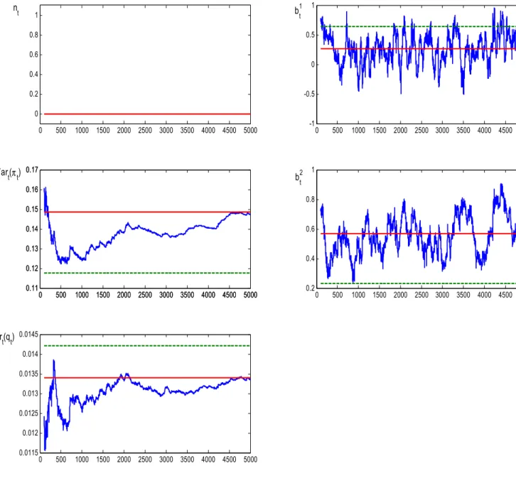
with θ = .6, γ0 = (.5, .75) κ = .01, λ = .04. We simulate the model, first with a transient period of length 15000, and then for 5000 periods in which we report the results in the figures below. To isolate the effect of parameter drift versus dual learning our strategy is as follows. We first present results where we fix the proportion of agentsnto one of its ME values, but allow agents to update their parameters with constant gain least squares. This is analogous to the approach pursued, for example, by Orphanides and Williams (2005a) in a full-information setting. We then present simulations with dual learning.
Figure 9 presents the results from a typical simulation. There are 5 panels in the figure. Beginning from the northwest and moving clockwise they are: predictor proportion n, belief parameters b1t, b2t, time t estimated unconditional variance of output and price respectively. The unconditional variances are computed as moving averages with window length 200 of the variance of the simulated time series. We set n = 0, though similar results obtain if we instead setn = 1. The horizontal lines in the figure are the ME values.
INSERT FIGURE 9 HERE
Figure 9 shows that some of the endogenous volatility can be attributed to para-meter drift. With a constant gain in the least-squares algorithm agents are sensitive
to structural change. This is why in the two panels on the right hand side of the fig-ure there is considerable parameter drift. This parameter drift manifests itself in the reduced-form parameters of the model and induces some endogenous volatility. How-ever, it does not generate the type of regime-shifting volatility that was documented in Section 2 and elsewhere in the literature.
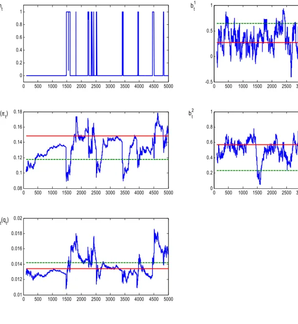
Figure 10 now puts both elements together to illustrate that dual learning can account for endogenous volatility. Figure 10 demonstrates combining parameter drift and dynamic predictor selection induces a stochastic process for inflation and output with volatility which both drifts and switches between high and low volatility regimes.
INSERT FIGURE 10 HERE
The length of time spent in a neighborhood of an ME depends in a complicated way on the size of the basin of attraction, the gains κ, λ, and the intensity of choice α. Figure 11 presents a ‘close-up’ view of a particular segment of the simulation in Figure 10. This segment clearly demonstrates the drifting and regime switching inflation and output volatility.
INSERT FIGURE 11 HERE
5.2
Further discussion
As a means of further discussion, an overview is helpful. We take a business cycle model where only unexpected shocks matter for real output fluctuations. We assume bounded rationality but preserve the spirit of Muth’s hypothesis and find that there exist multiple equilibria in a model with a unique REE. Moreover, these multiple equilibria arise because the self-referential feature of the Lucas model provides an incentive for agents to forecast with the same model. Each equilibrium can be char-acterized by the forecasting model that generates it, and each predictor produces distinct forecasts. For practical purposes, the important theoretical implication of the multiple equilibria result is that the self-referential property alters the effects the exogenous stochastic processes have on inflation and output; the positive feed-back from expectations onto inflation reinforces the effect of exogenous disturbances. As agents switch forecasting models, the underlying equilibrium stochastic process changes. This theoretical finding is the basis for the learning and predictor selection dynamics in this Section.
The model in this paper is an extension of the learning literature and Brock-Hommes’ Adaptively Rational Equilibrium Dynamics (A.R.E.D.). In the current paper beliefs and the choice of forecasting model are jointly determined. In contrast
to our earlier paper set in a cobweb model – whose primary distinction is a negative feedback from beliefs onto the state – we find multiple equilibria. This insight sug-gested, and our results confirm, that a dynamic version of the model can lead to new and important results.
Previous work by Orphanides and Williams (2005a) and Sargent (1999) highlight the role ‘perpetual learning’ might play in the Great Moderation. But, as has been argued elsewhere, the actual U.S. experience has been regime shifting and drifting volatility. The results of this section suggest a new avenue for exploring how an economy might endogenously generate shifting inflation and output volatility.
In particular, we identify two channels. Parameter learning with a constant gain version of least squares produces drifting volatility, but does not generate regime shift-ing volatility (Figure 9). However, the inclusion of constant gain dynamic predictor selection, in which agents estimate a geometric average of past squared forecast errors for each competing model, can lead to distinct shifts in inflation and output volatility (Figures 10-11). As with constant gain parameter updating, the use of constant gain in estimates of predictor fitness can be interpreted as a way of providing robustness against structural change.
With dual constant gain learning, shocks can occasionally lead agents to switch forecast models. This, via the feedback of expectations onto the state, produces a regime switch in inflation and output volatility that can have varying durations. Ev-idence presented in Cogley and Sargent (2005) and Sims and Zha (2005) suggest that drifting and regime switching volatility are important elements of the empirical record. The simulation results in this Section demonstrate that a simple self-referential eco-nomic model, in which agents choose between competing parsimonious predictors, provides a possible explanation for these findings. Future research should explore to what extent the implications of our theoretical model can account empirically for these characteristics of U.S. time series.
It is important to emphasize how natural the assumptions are that generate these results. We model agents as econometricians, in effect, taking the motivation of the learning literature seriously. Because of computational limitations and degrees of freedom problems agents are forced to underparameterize by omitting at least one variable and/or lag from their forecasting model. Although the agents are boundedly rational, they are ‘in the spirit’ of Muth’s original hypothesis since agents only select best-performing statistical models. In the real-time dynamic version of the model we again assume that agents behave as econometricians by recursively updating parame-ter and goodness of fit estimates in light of new data and remaining vigilant against structural change.
6
Conclusion
This paper has considered a simple Lucas-type monetary model in which inflation is driven by an exogenous process and by expectations of current inflation. We intro-duce model uncertainty and underparameterization to the framework. We assume that agents choose the best performing statistical models from a list of misspecified forecasting functions. When agents’ predictor choices are endogenous to the model, there exists an equilibrium for the stochastic process, agents’ beliefs, and the propor-tion of agents using a given model. Moreover, there may exist multiple Misspecifica-tion Equilibria, each with distinct stochastic properties. Numerical simulaMisspecifica-tions show that a subset of these equilibria are stable under least squares learning. If agents adopt dual learning with constant gains, then the system can endogenously switch between equilibria producing time-varying inflation and output volatility.
There is empirical evidence of time-varying inflation and GDP volatility that is consistent with the equilibrium and real-time learning properties of our model. Im-portantly, we identify two channels through which the economy may generate endoge-nously drifting and regime-switching economic volatility. The first channel is drifting parameter estimates that arise from an adaptive learning rule alert to possible struc-tural change. Drifting parameter estimates imply mean forecasts consistent with their equilibrium values, but with occasional departures that induce economic volatility not present in long-run equilibrium. The second channel is dynamic predictor selection. Analogously, predictor selection rules that remain alert to possible structural change can lead agents to switch forecast rules in response to occasional large shocks. Such shocks can induce switching between equilibria and produce persistent swings in in-flation and output volatility.
Our results show that endogenous volatility may arise naturally if underparameter-ization and positive expectational feedback are important elements of the economic process. Strikingly, we are able to obtain these results in a simple Lucas-model that has a unique rational expectations equilibrium. More generally, the results of this paper therefore indicate that there are potentially important implications from incorporating dual learning of parameter estimates and dynamic forecasting model selection.
A
Appendix
Proof of Proposition 3. The proof of the proposition follows Lemma 5 in Branch and Evans (2004). Here we briefly summarize the argument and amend it as necessary. We can rewrite (7) as
S(n1)ξ =A0γ,
whereξ0 = (ξ1, ξ2) and S(n1) is the indicated 2×2 matrix. We seek to signdF/dn1 =
(dF/dξ)0(dξ/dn1). Following Branch and Evans (2004) it can be verified that
dF/dn1 = 2θξ0K(n1)ξ, where K = 1−ρρ˜ 0 0 ρ2−Q S−1 1 ρ −˜ρ −1 = (r2−1)(−1+(1+n(r2−1))θ) (1−θ)+(n−1)n(r2−1)θ2 √ Qr(r2−1)(θ−1) (1−θ)+(n−1)n(r2−1)θ2 √ Qr(r2−1)(θ−1) (1−θ)+(n−1)n(r2−1)θ2 −Q(r2−1)(1−r2θ+n(r2−1)θ) (1−θ)+(n−1)n(r2−1)θ2
Here r2 =ρρ˜with 0≤ r2 <1. Notice that K is symmetric. It is easily verified that
the necessary and sufficient condition for monotonicity thatK is positive semidefinite is satisfied.
Proof of Proposition 5. Our proof again follows Branch and Evans (2004). In our earlier paper it was established that for eachα the mapTα has a fixed point denoted
n∗(α), and, moreover, ∃{α(s)}s s.t. α(s) → ∞ ⇒ n(α(s)) → n¯ for some ¯n which is
a fixed point to the map limα(s)→∞Tα(s). The proposition claims that ¯n ∈ {0,n,ˆ 1}
where F(ˆn) = 0. That ˆn is a fixed point was proven in Proposition 8 of Branch and Evans (2004). Following the arguments for Conditions P0 and P1 in that proposition, it is clear that F0 >0 implies ¯n ∈ {0,1} is a fixed point.
References
[1] Adam, Klaus, 2005a,“Learning to Forecast and Cyclical Behavior of Output and Inflation,”Macroeconomic Dynamics, 9, 1, 1-27.
[2] Adam, Klaus, 2005b, “Experimental Evidence on the Persistence of Output and Inflation,” mimeo.
[3] Bernanke, Ben S., and Ilian Mihov, 1998, “Measuring Monetary Policy,” Quar-terly Journal of Economics, 113, 3, 869-902.
[4] Branch, William A., and George W. Evans, 2005,“A Simple Recursive Forecast-ing Model,” forthcomForecast-ing Economics Letters.
[5] Branch, William A., John Carlson, George W. Evans, and Bruce McGough, 2004, “Monetary Policy, Endogenous Inattention, and the Volatility Trade-off,” mimeo.
[6] Branch, William A., and George W. Evans, 2004, “Intrinsic Heterogeneity in Expectation Formation,” forthcoming Journal of Economic Theory.
[7] Branch, William A., and Bruce McGough, 2005, “Misspecification and Consis-tent Expectations in Stochastic Non-linear Economies,” Journal of Economic
Dynamics and Control, 29, 659-676.
[8] Brock, William A., and Cars H. Hommes, 1997, “A Rational Route to Random-ness”, Econometrica, 65, 1059-1160.
[9] Brock, William A., and Cars H. Hommes, 1998, “Heterogeneous Beliefs and Routes to Chaos in a Simple Asset Pricing Model,” Journal of Economic
Dy-namics and Control, 22, 1235-1274.
[10] Bullard, James, and In Koo Cho, 2005, “Escapist Policy Rules,” Journal of
Economic Dynamics and Control, 29, 1841-1865.
[11] Chari, V.V. Patrick J. Kehoe, and Ellen R. McGrattan, 2005, “A Critique of Structural VARs Using Real Business Cycle Theory,” FRB-Minneapolis W.P. 631.
[12] Cho, In Koo, and Ken Kasa, 2002, “Learning Dynamics and Endogenous Cur-rency Crises,” mimeo.
[13] Cho, In Koo, Noah Williams and Thomas J. Sargent, 2002, “Escaping Nash Inflation,”Review of Economic Studies, 69, 1-40.
[14] Cogley, Timothy W., and Thomas J. Sargent, 2005, “Drifts and Volatilities: Monetary Policies and Outcomes in the Post WWII U.S.,” Review of Economic
Dynamics,8.
[15] Evans, George, W., and Seppo Honkapohja, 1993, “Adaptive Expectations, Hys-teresis and Endogenous Fluctuations,” Federal Reserve Bank of San Francisco
Economic Review, 1993,1, 3-13.
[16] Evans, George W., and Seppo Honkapohja, 2001, Learning and Expectations in
Macroeconomics, Princeton University Press, Princeton, NJ.
[17] Evans, George W., Seppo Honkapohja, and Thomas J. Sargent, 1989, “On the Preservation of Deterministic Cycles when Some Agents Perceive Them to be Random Fluctuations,” Journal of Economic Dynamics and Control, 17, 705-721.
[18] Evans, George W., and Garey Ramey, 1992. “Expectation Calculation and Macroeconomic Dynamics,” American Economic Review, 82,1, 207-224.
[19] Evans, George W., and Garey Ramey, 2004. “Adaptive Expectations, Underpa-rameterization and the Lucas Critique,” University of Oregon Economic Depart-ment Working Paper 2001-8, revised Dec. 2004, forthcomingJournal of Monetary Economics.
[20] Guse, Eran, 2005, “Stability Properties for Learning with Heterogeneous Expec-tations and Multiple Equilibria,” Journal of Economic Dynamics and Control, 29, 1623-1642.
[21] Hansen, Lars Peter, and Thomas J. Sargent, 2005, Misspecification in Recursive
Macroeconomic Theory, manuscript.
[22] Hommes, Cars, and Gerhard Sorger, 1998, “Consistent Expectations Equilibria,”
Macroeconomic Dynamics, 2, 287-321.
[23] Hommes, Cars, Gerhard Sorger, and Florian Wagener, 2002, “Learning to Believe in Linearity in an Unknown Nonlinear Stochastic Economy,” mimeo.
[24] Horn, Roger A., and Charles R. Johnson, 1985, Matrix Analysis, Cambridge University Press, Cambridge.
[25] Kasa, Kenneth, 2004, “Learning, Large Deviations, and Recurrent Currency Crises,” International Economic Review, 45, 141-173.
[26] Kim, Chang-Jin, and Charles Nelson, 1999, “Has the U.S. Economy Become More Stable? A Bayesian Approach Based on a Markov-Switching Model of the Business Cycle” Review of Economics and Statistics, 81, 4, 608-616.
[27] Kim, Chang-Jin, Charles Nelson, and Jeremy Piger, 2004, “The Less Volatile U.S. Economy: A Bayesian Investigation of Timing, Breadth, and Potential Explanations,” Journal of Business and Economic Statistics, 22, 1, 80-93. [28] Manski, Charles F., and Daniel McFadden, 1981, Structural Analysis of Discrete
Data with Econometric Applications, MIT Press, Cambridge, MA.
[29] McGough, Bruce, 2004, “Shocking Escapes,” Economic Journal, forthcoming. [30] Marcet, Albert, and Juan Pablo Nicolini, 2003, “Recurrent Hyperinflation and
Learning,” American Economic Review, 93,5, 1476-1495.
[31] Marcet, Albert, and Thomas J. Sargent, 1989, “Convergence of Least-Squares Learning Mechanisms in Self-Referential Linear Stochastic Models,” Journal of
Economic Theory, 48, 337-368.
[32] Marcet, Albert, and Thomas J. Sargent, 1995, “Speed of Convergence of Recur-sive Least Squares: Learning with AutoregresRecur-sive Moving-Average Perceptions,”
inLearning and Rationality in Economics, eds. A. Kirman and M. Salmon, Basil
Blackwell, Oxford, 179-215.
[33] McConnell, Margaret, and Gabriel Perez Quiros, 2000, “Output Fluctuations in the United States: What has Changed Since the Early 1980’s?” American
Economic Review, 1464-1476.
[34] Milani, Fabio, 2005, “Expectations, Learning, and Macroeconomic Persistence,” mimeo.
[35] Muth, John F., 1961, “Rational Expectations and the Theory of Price Move-ments,” Econometrica, 29, 315-335.
[36] Orphanides, Athanasios, and John C. Williams, 2005a, “Imperfect Knowledge, Inflation Expectations, and Monetary Policy,” Chapter 5 in Inflation Target-ing, ed. Ben S. Bernanke and Michael Woodford, National Bureau of Economic Research and University of Chicago Press, Chicago.
[37] Orphanides, Athanasios, and John C. Williams, 2005b, “The Decline of Activist Stabilization Policy: Natural Rate Misperceptions, Learning and Expectations,”
Journal of Economic Dynamics and Control, 29, 1927-1950.
[38] Owyang, 2001, “Persistence, Excess Volatility, and Volatility Clusters in Infla-tion,” Federal Reserve Bank of St. Louis Review, Nov./Dec., 41-52.
[39] Sargent, Thomas J., 1991,Bounded Rationality in Macroeconomics, Oxford Uni-versity Press, Oxford.
[40] Sargent, Thomas J., 1999, The Conquest of American Inflation, Princeton Uni-versity Press, Princeton, NJ.
[41] Sensier, Marianne, and Dick van Dijk, 2004, “Testing For Changes in Volatility of US Macroeconomic Time Series”, Review of Economics and Statistics, 86, 833-839.
[42] Sims, Christopher A., and Tao Zha, 2005, “Were There Regime Switches in US Monetary Policy?,” forthcoming American Economic Review.
[43] Stock, James, and Mark W. Watson, 2003, “Has the Business Cycle Changed? Evidence and Explanations”, forthcomingFRB Kansas City symposium, Jackson Hole, Wyoming, August 28-30, 2003.
[44] Williams, Noah, 2004a, “Escape Dynamics in Learning Models,” mimeo.
[45] Williams, Noah, 2004b, “Stability and Long-Run Equilibrium in Stochastic Fic-titious Play,” mimeo.
[46] Woodford, Michael, 2003, Interest and Prices, Princeton University Press, Princeton NJ.
-5 0 5 10 15 1950 1960 1970 1980 1990 2000 Inflation -10 -8 -6 -4 -2 0 2 4 6 1950 1960 1970 1980 1990 2000 GDP Growth
0
10
20
30
40
1950
1960
1970
1980
1990
2000
Moving Average Inflation
Moving Average log GDP
Figure 2. Moving Averages (with window length of 8 quarters) of unconditional variance of inflation and detrended log GDP.
0 5 10 15 20 25 30 35 1950 1960 1970 1980 1990 2000
Conditional Variance Inflation
0.0 0.4 0.8 1.2 1.6 2.0 2.4 2.8 3.2 1950 1960 1970 1980 1990 2000
Conditional Variance log GDP
Figure 3. Conditional Variances from a GARCH(1,1) model of an AR(4) process for Inflation and log GDP. Sample: 1947:1-2004:2.
0
1
2
3
4
5
55
60
65
70
75
80
85
90
95
00
Conditional Variance Inflation
Conditional Variance log GDP
Figure 4. Conditional Variances from a GARCH(1,1) model of an AR(4) process for Inflation and log GDP. Sample: 1955:1-2004:2.
0 0.1 0.2 0.3 0.4 0.5 0.6 0.7 0.8 0.9 1 0 0.1 0.2 0.3 0.4 0.5 0.6 0.7 0.8 0.9 1 n Tα(n) 0 0.1 0.2 0.3 0.4 0.5 0.6 0.7 0.8 0.9 1 -1.4 -1.2 -1 -0.8 -0.6 -0.4 -0.2 0 0.2 n F(n) Large α Small α