Decomposition algorithms for the tree edit
distance problem
Serge Dulucq
a, Hélène Touzet
b,∗aLaBRI, UMR CNRS 5800, Université Bordeaux I, 33 405 Talence cedex, France bLIFL, UMR CNRS 8022, Université Lille 1, 59 655 Villeneuve d’Ascq cedex, France
Available online 21 September 2004
Abstract
We study the behavior of dynamic programming methods for the tree edit distance problem, such as [P. Klein, Computing the edit-distance between unrooted ordered trees, in: Proceedings of 6th European Symposium on Algorithms, 1998, p. 91–102; K. Zhang, D. Shasha, SIAM J. Comput. 18 (6) (1989) 1245–1262]. We show that those two algorithms may be described as decomposition strategies. We introduce the general framework of cover strategies, and we provide an exact char-acterization of the complexity of cover strategies. This analysis allows us to define a new tree edit distance algorithm, that is optimal for cover strategies.
2004 Elsevier B.V. All rights reserved.
Keywords: Algorithm; Edit distance; Alignment; Tree; Computational biology
1. Introduction
Many processes can be described as transformations of ordered trees. Examples include the analysis of hierarchically structured data [1], such as XML documents, or compari-son of RNA secondary structures in computational biology [8]. One way of comparing two ordered trees is by measuring their edit distance: the minimum cost to transform one tree into another using elementary operations. There are many variants of tree edit dis-tance: alignment[4], constrained edit distances[1,7,14], distance with non-linear gap costs
*Corresponding author.
E-mail addresses:[email protected](S. Dulucq),[email protected](H. Touzet). 1570-8667/$ – see front matter 2004 Elsevier B.V. All rights reserved.
[10], . . . . We focus here on the general editing problem: insertions and deletions may take place in any order at any node within the tree. In 1979, Tai[9]introduced an algorithm for this problem with run time in O(n6). Many others solution have been designed, based on back tracking, divide-and-conquer, . . . (see[11]for a survey). Amongst these paradigms, dynamic programming appears to be a fruitful approach. There are currently two main dy-namic programming algorithms for solving the tree edit distance problem: Zhang–Shasha’s [13]and Klein’s[5]. Both algorithms may be seen as an extension of the basic string edit distance algorithm. The difference lies in the set of sub-forests that are involved in the de-composition. This leads to different complexities: Zhang–Shasha is in O(n4)in worst case, as Klein is in O(n3log(n)). However, this does not mean that Klein’s approach is strictly better than Zhang–Shasha’s. Depending on the input trees, Zhang and Shasha’s algorithm may be faster. The performance of each algorithm depends on the shape of the two trees to be compared.
The purpose of this paper is to present a general analysis of dynamic programming for tree edit distance algorithms. For that, we introduce a class of tree decompositions, called cover strategies, which involves Zhang–Shasha and Klein algorithms. We study the complexity of those decompositions by counting the exact number of distinct recursive calls for the underlying corresponding algorithm. As a corollary, this gives the number of recursive calls for Zhang–Shasha, that was a known result[13], and for Klein, that was not known. In the last section, we take advantage of this analysis to define a new edit distance algorithm for trees, which improves Zhang–Shasha and Klein algorithms with respect to the number of recursive calls.
2. Edit distance for trees and forests 2.1. Definitions
Definition 1 (Trees and forests). A tree is a node (called the root) connected to an ordered sequence of disjoint trees. Such a sequence is called a forest. We write(A1◦ · · · ◦An)for the tree composed of the nodeconnected to the sequence of treesA1, . . . , An.
This definition assumes that trees are ordered trees, and that the nodes are labeled. When it is clear from the context, we shall not distinguish between a node and its label. Trees with labeled edges can by handled similarly. In the sequel, we may use the word forest for denoting both forests and trees, a tree being a sequence reduced to a single element. We introduce some classical notations for trees and forests.
Notation 1. LetF be a forest.
• |F|denotes the size ofF, that is the number of nodes of the forestF,
• #leaves(F )denote the number of leaves ofF,
• height(F )denotes the height ofF, that is the maximal height of the trees compos-ingF,
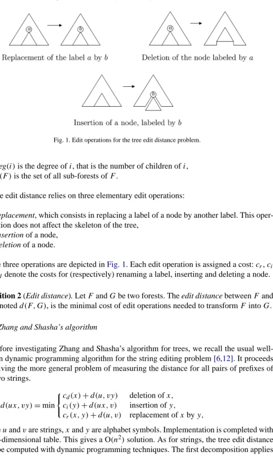
Fig. 1. Edit operations for the tree edit distance problem.
• deg(i)is the degree ofi, that is the number of children ofi,
• F(F )is the set of all sub-forests ofF.
The edit distance relies on three elementary edit operations:
• replacement, which consists in replacing a label of a node by another label. This oper-ation does not affect the skeleton of the tree,
• insertion of a node,
• deletion of a node.
Those three operations are depicted inFig. 1. Each edit operation is assigned a cost:cr,ci andcddenote the costs for (respectively) renaming a label, inserting and deleting a node.
Definition 2 (Edit distance). LetF andGbe two forests. The edit distance betweenF and
G, denotedd(F, G), is the minimal cost of edit operations needed to transformF intoG.
2.2. Zhang and Shasha’s algorithm
Before investigating Zhang and Shasha’s algorithm for trees, we recall the usual well-known dynamic programming algorithm for the string editing problem[6,12]. It proceeds by solving the more general problem of measuring the distance for all pairs of prefixes of the two strings.
d(ux, vy)=min c
d(x)+d(u, vy) deletion ofx,
ci(y)+d(ux, v) insertion ofy,
cr(x, y)+d(u, v) replacement ofxbyy,
whereuandvare strings,xandyare alphabet symbols. Implementation is completed with a two-dimensional table. This gives a O(n2)solution. As for strings, the tree edit distance may be computed with dynamic programming techniques. The first decomposition applies
necessarily to the roots of the trees: (1) d(f ), (g)=min cd()+d(f, (g)) deletion of, ci()+d((f ), g) insertion of, cr(, )+d(f, g) replacement ofby.
We now have to solve the problem for forests. Deletion and insertion cases are similar to the recurrence formulae for strings. Replacement generates two novel recursive calls: one call for the subtrees of the replaced node, that have to match together, and one call for the remaining nodes of the forests.
(2) dt◦(f ), v◦(g)=min cd()+d(t◦f, v◦(g)) deletion of, ci()+d(◦(f ), v◦g) insertion of, d((f ), (g))+d(t, v) replacement ofby.
The sub-forests that can occur in the recursion are either subtrees, or prefixes of subtrees. We name it leftmost forests.
Definition 3 (Leftmost forests). LetAbe a tree. The set of leftmost sub-forests of Ais the least set satisfying
• for each nodeiofA,A(i)is a leftmost forest,
• ift◦(g)is a leftmost sub-forest, thent◦gis a leftmost sub-forest too. We write#left(A)for the number of leftmost sub-forests ofA.
The number of leftmost sub-forests of A is bounded byn(n+1)/2, where n is the size ofA. It is possible to get a better majorization of that value with the definition of the collapsed depth.
Definition 4 (Collapsed depth [13]). Let A be a tree. The set keyroots(A) is de-fined as keyroots(A)= {root(A)} ∪ {i∈A, ihas a left sibling}. For each node i of A, collapsed_depth(i)is the number of keyroot ancestors ofiand
collapsed_depth(A)=maxcollapsed_depth(i), i∈A.
Proposition 5[13]. For any treeA,#left(A)|A| ×collapsed_depth(A).
This proposition yields an upper bound in O(n4)for Zhang–Shasha’s algorithm. This result appears to be a least upper bound in the worst case. Consider filiform binary treesbn of size 2n+1: each internal nodes has exactly two children and he leftmost child is a leaf. That isb1= •andbn+1= •(• ◦bn). The number of leftmost sub-forests is(2n2+1)for a tree and so the number of sub-forests for the pair of trees is in O(n4).
However the average complexity is better. It can be shown that|A|×collapsed_depth(A)
|A|min(#leaves(A),height(A)), and the average complexity is in O(n3)[2]. We introduce now a variation of Zhang–Shasha’s algorithm, that comes from a simple but crucial remark. For string edit distance, it is likely to develop an alternative dynamic
programming algorithm by constructing the distance for all pairs of suffixes. This gives the following recursive relationship:
d(xu, yv)=min c
d(x)+d(u, yv) deletion ofx,
ci(y)+d(xu, v) insertion ofy,
cr(x, y)+d(u, v) replacement ofx byy.
The same point of view is applicable to trees and forests. A forest can be decomposed from the left instead of being decomposed from the right.
(3) d(f )◦t, (g)◦v=min cd()+d(f ◦t, (g)◦v) deletion of, ci()+d((f )◦t, g◦v) insertion of, d((f ), (g))+d(t, v) replacement ofby.
This alternative recursive scheme is based on suffixes and suffixes of subtrees. It gives rise to rightmost forests.
Definition 6 (Rightmost forests). LetAbe a tree. The set of rightmost sub-forests ofAis the least set satisfying
• for each nodeiofA,A(i)is a rightmost forest,
• if(g)◦tis a rightmost sub-forest, theng◦tis a rightmost sub-forest too. We write#right(A)for the number of rightmost sub-forests ofA.
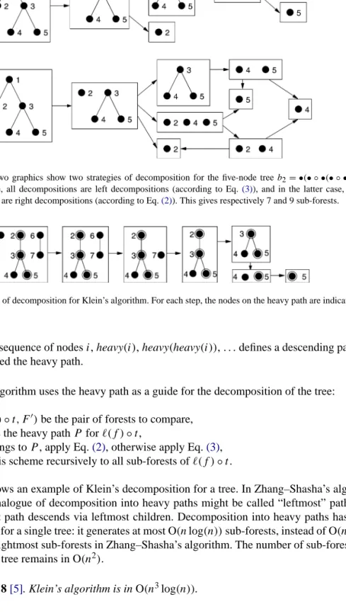
We call decomposition according to Eq. (2), involving leftmost forests, a right de-composition, and decomposition according to Eq. (3), involving rightmost forests, a left decomposition. In the sequel, we use the word direction to indicate that the decomposition is left or right. For strings, left and right decompositions are equivalent, since the number of pairs of prefixes equals the number of pairs of suffixes. This equivalence is no longer valid for tree edit distance. The choice between Eqs.(2) and (3)may lead to different numbers of recursive calls. The asymptotic and average complexity of both algorithms, measured by the number of rightmost or leftmost sub-forests, are of course identical. However, when you analyze trees individually, it can induce a significant difference, due to the shape of the tree. For example, for the family of filiform binary trees, each treebngenerates 3n+1 rightmost sub-forests only.Fig. 2shows all leftmost and rightmost sub-forests forn=2. So when you compute the distanced(bn, bn), the complexity decreases from O(n4)to O(n2) for this example. This remark is the basis for the definition of Klein’s algorithms.
2.3. Klein’s algorithm
Klein’s algorithm brings two new ideas: alternating the directions of decomposition in the dynamic programming scheme, and adding the employment of a tree decomposition into heavy paths. The concept of heavy paths was introduced by Harel and Tarjan[3]. Definition 7 (Heavy paths[3]). Given a rooted treeA, define the weight of each nodeiofA
Fig. 2. These two graphics show two strategies of decomposition for the five-node treeb2= •(• ◦ •(• ◦ •)). In the first case, all decompositions are left decompositions (according to Eq.(3)), and in the latter case, all decompositions are right decompositions (according to Eq.(2)). This gives respectively 7 and 9 sub-forests.
Fig. 3. Example of decomposition for Klein’s algorithm. For each step, the nodes on the heavy path are indicated by circles.
weight. The sequence of nodesi, heavy(i), heavy(heavy(i)),. . .defines a descending path which is called the heavy path.
Klein’s algorithm uses the heavy path as a guide for the decomposition of the tree: (1) let((f )◦t, F)be the pair of forests to compare,
(2) compute the heavy pathP for(f )◦t,
(3) ifbelongs toP, apply Eq.(2), otherwise apply Eq.(3), (4) apply this scheme recursively to all sub-forests of(f )◦t.
Fig. 3shows an example of Klein’s decomposition for a tree. In Zhang–Shasha’s algo-rithm, the analogue of decomposition into heavy paths might be called “leftmost” paths. The leftmost path descends via leftmost children. Decomposition into heavy paths has a great benefit for a single tree: it generates at most O(nlog(n))sub-forests, instead of O(n2)
leftmost or rightmost sub-forests in Zhang–Shasha’s algorithm. The number of sub-forests for the other tree remains in O(n2).
Fig. 4.(A, B).
Proposition 8 does not mean that Klein’s approach is always better than Zhang– Shasha’s. Depending on the input trees, Zhang and Shasha’s algorithm may be faster. For example, for the pair of trees(A, B)ofFig. 4, Klein’s approach needs 84 distinct recursive calls, whereas the Zhang–Shasha’s approach needs only 72 distinct recursive calls.
The reason comes from the asymmetrical construction of Klein’s algorithms. Only one tree is affected by the heavy path decomposition. The number of sub-forests for the second tree may be greater for Klein’s algorithm than for Zhang–Shasha’s. This is the price to pay for the clever decomposition of the first tree.
3. Decomposition strategies
To make the definition of alternation of Eqs. (2) and (3) more formal, we introduce the framework of decomposition strategies. We then give several general properties of decomposition strategies.
Definition 9 (Strategy). LetF andGbe two forests. A strategy is a mapping fromF(F )×
F(G)to{left,right}.
Each strategy is associated with a specific set of recursive calls. We name relevant forests the forests that are involved in these recursive calls. This terminology is adapted from[5], where it is used for a single tree. We consider here relevant forests for the whole pair of trees.
Definition 10 (Relevant forests). Let(F, G)be a pair of forests provided with a strategyφ. The setR(F, G)of relevant forests is defined as the least subset ofF(F )×F(G)such that if the decomposition of(F, G)meets the pair(F, G), then(F, G)belongs toR(F, G). For instance, for Zhang–Shasha’s algorithm, the set of relevant forests is the set of leftmost forests.
Lemma 11. Let(F, F)be a pair of forests provided with a strategyφ. The setR(F, F)
of relevant forests satisfies:
•IfF orFis an empty forest:
Rε, (g)◦t=(ε, (g)◦t )∪R(ε, g◦t ) wheneverφε, (g)◦t=left,
Rε, t◦(g)=ε, t◦(g)∪R(ε, t◦g) wheneverφε, t◦(g)=right,
Rt◦(g), ε=t◦(g), ε∪R(t◦g, ε) wheneverφt◦(g), ε=right,
R(ε, ε)= ∅.
•If(F, F)=((g)◦t, (h)◦u)andφ(F, F)=left, thenR(F, F)is
(F, F)∪R(g◦t, F)∪R(F, h◦u)∪R(g), (h)∪R(t, u)
•If(F, F)=(t◦(g), u◦(h))andφ(F, F)=right, thenR(F, F)is
(F, F)∪R(t◦g, F)∪R(F, u◦h)∪R(g), (h)∪R(t, u).
Proof. By induction on|F| + |F|, using Eqs.(1), (2) and (3). 2
We writeR(F )andR(G)to denote the projection ofR(F, G)onF(F )andF(G) re-spectively.
Lemma 12.
R(g)=(g)∪R(g) no matter what the direction is,
R(g)◦t=(g)◦t∪R(g◦t )∪R(g)∪R(t ) if the direction is left,
Rt◦(g)=t◦(g)∪R(t◦g)∪R(g)∪R(t ) if the direction is right.
Proof. Straightforward implication ofLemma 11. 2
Lemma 13. LetF andGbe two forests. For any strategyφ, for any nodesiofF andj of
G,(F (i), G(j ))is an element ofR(F, G).
Proof. By induction on the size ofF andG. 2
Given a decomposition strategy, the number of relevant sub-forests is a measure of the complexity of the associated edit distance algorithm.
Notation 2. We denote#relthe number of relevant forests:
• #rel(F, G)is the cardinality ofR(F, G),
• #rel(F )is the cardinality ofR(F ).
Lemma 14. Given a treeA=(A1◦ · · · ◦An), for any strategy we have
#rel(A)|A| − |Ai| +#rel(A1)+ · · · +#rel(An), wherei∈ [1..n]is such that the size ofAi is maximal.
Proof. LetF=A1◦ · · · ◦An. We first prove that
(4) #rel(F )|F| − |Ai| +#rel(A1)+ · · · +#rel(An).
The proof is by induction onn. Ifn=1, then the result is direct. Ifn >1, assume that a left operation is applied toF (the other case with a right operation is identical). Let,g,t
such thatA1=(g)andt=A2◦ · · · ◦An. ByLemma 12, we have
(5) R(F )= {F} ∪R(A1)∪R(T )∪R(g◦t ).
It is possible to prove by induction on|g| + |t|that the number of relevant forests ofg◦t
containing both nodes of gand nodes oft is greater than min{|g|,|t|}. Therefore Eq.(5) implies
(6) #rel(F )1+#rel(A1)+#rel(t )+min
|g|,|t|.
Letj∈ [2..n]such thatAj has the maximal size among{A2, . . . , An}. Applying induction hypothesis fort, we have#rel(t )|t| − |Aj|+#rel(A2)+ · · · +#rel(An). So Eq.(6) becomes
(7) #rel(F )1+#rel(A1)+ · · · +#rel(An)+ |t| − |Aj| +min
|g|,|t|.
To establish Eq.(4), it remains to verify that
(8) 1+ |t| − |Aj| +min
|g|,|t||F| − |Ai|.
There are two cases, depending on the size of gandt. In the first case, if|g||t|, then 1+ |t| +min{|g|,|t|} = |F|. Since |Aj||Ai|, it follows that 1+ |t| +min{|g|,|t|} −
|Aj||F| − |Ai|. In the latter case, if |t|<|g|, thenA1 is the largest subtree ofA. So
i=1 and|F| − |Ai| = |t|, that implies 1+ |t| − |Aj| +min{|g|,|t|}|F| − |Ai|. We now show how Eq. (4) gives the expected result. ByLemma 12again, we have R(A)= {A} ∪R(F ). Hence
#rel(A)=1+#rel(F )
1+ |F| − |Ai| +#rel(A1)+ · · · +#rel(An) (Eq.(4))
= |A| +#rel(A1)+ · · · +#rel(An). This concludes the proof. 2
Lemma 15. For every natural numbern, there exists a treeAof sizensuch that for any strategy,#rel(A)has a lower bound in O(nlog(n)).
Proof. LetTn be a complete balanced binary tree of sizen. We prove by induction onn that
(9) #rel(Tn)
(n+1)log2(n+1)
2 .
– Ifn=1, then#rel(Tn)=1, that is consistent with Eq.(9).
– If n >1, let m=(n−1)/2. Tn is of the form(A◦B), where A andB are two complete balanced trees of sizem. ByLemma 14, we have
By induction hypothesis forTm, it follows that #rel(Tn)n−m+(m+1)log2(m+1) (n+1)(log2(m+1)+1) 2 =(n+1)log2(2m+2) 2 =(n+1)log2(n+1) 2 . 2
Corollary 16. Let A and B be two trees of size n. For any decomposition strategy,
#rel(A, B)has a lower bound in O(n2log2(n)).
4. Cover strategies
In this section, we define a main family of strategies that we call cover strategies. The idea comes from the following remark. Assume that (f )◦f is a relevant forest for a given strategy. Suppose that the direction of(f )◦tis left. This decomposition generates three relevant forests:(f ),tandf◦t. The forestf is a sub-forest off◦t. An opportune point of view is then to first eliminate nodes off inf◦t, so thatf◦t andtshare relevant forests as most as possible. We make this intuitive property more formal by defining covers. Covers are generalization of path decompositions.
Definition 17 (Cover). LetF be a forest. A coverr ofF is a mapping from F toF ∪
{right,left}satisfying for each nodeiinF
• if deg(i)=0 or deg(i)=1, thenr(i)∈ {right,left};
• if deg(i) >1, thenr(i)is a child ofi.
In the first case,r(i)is called the direction ofi, and in the latter case,r(i)is called the favorite child ofi.
Definition 18 (Cover strategy). Given a pair of trees(A, B)and a coverrforA, we asso-ciate a unique strategyφas follows:
• if deg(i)=0 or deg(i)=1, thenφ(A(i), G)=r(i), for each forestGofB.
• ifA(i)is of the form(A1◦ · · · ◦An)withn >1, then letp∈ {1, . . . , n}such that the favorite childr(i)is the root ofAp. For each forestGofB, we define
φA(i), G=right wheneverp=1, left otherwise,
φ(T◦Ap◦ · · · ◦An, G)=left, for each forestT ofA1◦ · · · ◦Ap−1,
The treeAis called the cover tree. A strategy is a cover strategy if there exists a cover associated to it.
The family of cover strategies includes Zhang–Shasha and Klein algorithms. The Zhang–Shasha algorithm corresponds to the cover
• for any node of degree 0 or 1, the direction is right,
• for any other node, the favorite child is the leftmost child.
The associated strategy involves only right decomposition rules, according to Eq. (2). Klein’s algorithm may be described as the cover strategy
• for any node of degree 0 or 1, the direction is left,
• for any other node, the favorite child is the root of the heaviest subtree.
The aim is now to study the number of relevant forests for a cover strategy. This task is divided into two steps. First, we compute the number of strategies for the cover tree alone. This intermediate result will play a great part in our final objective.
Lemma 19. Letf be a forest,t a nonempty forest anda labeled node.
• Letφ be a cover strategy for (f )◦t such thatφ((f )◦t )=left, letk= |f|. We writef1, . . . , fk for denoting theksub-forests of f corresponding to the successive left decompositions off:f1isf, and eachfi+1is obtained fromfiby a left deletion.
R(f )◦t=(f )◦t, f1◦t, . . . , fk◦t
∪R(f )∪R(t ).
• Letφbe a cover strategy fort◦(f )such thatφ(t◦(f ))=right, letk= |f|. We writeg1, . . . , gk for denoting thek sub-forests off corresponding to the successive right decompositions of f: g1 is f, and each gi+1 is obtained fromgi by a right deletion.
Rt◦(f )=t◦(f ), t◦g1, . . . , t◦gk
∪R(f )∪R(t ).
Proof. We show the first claim, the proof of the other one being symmetrical. By Lemma 11, we have
(10) R(f )◦t=(f )◦t∪R(f )∪R(t )∪R(f◦t ).
Let’s have a closer look atf ◦t. We establish that
(11) R(f◦t )= {f1◦t} ∪ · · · ∪ {fk◦t}
i∈f
Rf (i)∪R(t ).
The proof is by induction onk. Ifk=1, thenf =f1andR(f◦t )= {f1◦t} ∪R(t ), that is the expected result. Ifk >1, let,fandtsuch thatf=(f)◦t. We have
On the other handF =f1,f◦t=f2andt=f|(f)|+1. Sinceφis a cover strategy, the direction forf◦tand for successive sub-forests containingtis left. We apply the induction hypothesis totandf◦tand it concludes the proof of Eq.(11).
We come back to Eq.(10). With Eq.(11), we get R(f )◦t=(f )◦t∪ {f1◦t} ∪ · · · ∪ {fk◦t}
i∈f
Rf (i)∪R(f )∪R(t ).
According toLemma 13, for each nodeiinf,R(f (i))is included inR((f )). It follows that
R(f )◦t=(f )◦t∪ {f1◦t} ∪ · · · ∪ {fk◦t} ∪R
(f )∪R(t ). 2
The first consequence of this lemma is that cover strategies can reach the O(nlog(n))
lower bound ofLemma 15. We give a criterion for that.
Lemma 20. Let F be a forest provided with a cover strategyφ, satisfying the following property: for each relevant forestA◦t◦B(AandBare trees,tis a forest)
• if|B|>|A◦t|, thenφ(A◦t◦B)=left, and
• if|A|>|t◦B|, thenφ(A◦t◦B)=right, then#rel(F )|F|log2(|F| +1).
Proof. The proof is by induction on the sizeF. – IfF is empty, the result is direct.
– IfF is a single tree:F is of the form(g), and#rel(F )=1+#rel(g). By induction hypothesis forg,#rel(g)|g|log2(|g| +1). Since |F| = |g| +1, it follows that #rel(F )|F|log2(|F| +1).
– IfF is not a single tree, there are two nonempty treesAandBand a, possibly empty, foresttsuch thatF =A◦t◦B. Assumeφ(F )=left (the caseφ(F )=right is identi-cal). Letn= |A|andm= |t◦B|. ByLemma 19,
(12) #rel(F )=n+#rel(A)+#rel(t◦B).
By induction hypothesis forAandt◦B, it follows that#rel(F )n+nlog2(n+
1)+mlog2(m+1).Sinceφ(F )=left, the hypothesis of the lemma implies thatnm
and so#rel(F )(n+m)log2(n+m+1). 2
Another application of Lemma 19is that it is possible to know the exact number of relevant forests for the cover tree.
Lemma 21. LetA=(A1◦ · · · ◦An)be a cover tree such thatn=1 or the root ofAj is the favorite child.
R(A)= {A} ∪ {f1, . . . , fk} ∪ {g1, . . . , gh} i
wherekis the size ofA1◦ · · · ◦Aj−1,his the size ofAj+1◦ · · · ◦An,f1isA1◦ · · · ◦An,
and eachfi+1is obtained fromfi by a left deletion,g1isAj◦ · · · ◦Anand eachgi+1is
obtained fromgi by a right deletion.
Proof. The proof is by induction on the size ofA. If|A| =1, thenR(A)is{A}. If|A|>1, byLemma 11,R(A)is{A} ∪R(A1◦ · · · ◦An). Iterated application ofLemma 19yields the expected result. 2
Lemma 22. LetA=(A1◦ · · · ◦An)be a cover tree such thatn=1 or the root ofAj is the favorite child.
#rel(A)= |A| − |Aj| +#rel(A1)+ · · · +#rel(An). Proof. Direct consequence ofLemma 21. 2
Remark 23. As a corollary ofLemma 22andLemma 14, we know that Klein’s algorithm is a strategy that minimizes the number of relevant forests for the cover tree, andLemma 20 implies that the number of relevant forests for the cover tree is in O(nlog(n)). Together withLemma 35, this gives a new, simpler proof ofProposition 8concerning the class of complexity of Klein’s algorithm.
With the analysis of the number of relevant forests for the cover tree, we are now able to look for the total number of relevant forests for a pair of trees. Given a pair of trees
(A, B)provided with a cover forA, it appears that all relevant forests ofAfall within three categories:
(α) those that are compared with all rightmost forests ofB, (β) those that are compared with all leftmost forests ofB, (γ) those that are compared with all special forests ofB.
Definition 24 (Special forests). LetF be a tree. The setS(F )of special forests ofF is the set of sub-forests that can deduced fromF by a series of right or left deletions.
S(f )◦t◦(g)=(f )◦t◦(g)Sf◦t◦(g)∪S(f )◦t◦g.
We write#spec(A)for the number of special forests ofA.
Lemma 25. For any forestF, for any strategyφ, the set of relevant forestsR(F )is included in the set of special forests ofS(F ).
Proof. By induction on|F|. 2
The goal of the next lemmas is to find criteria to assign the proper category(α),(β)or
(γ )to each relevant forest ofA. We have this immediate result.
Lemma 26. Let (A, B)be a pair of trees, Abeing a cover tree, and letf be a relevant forest ofA:
• if the direction off is left, thenf is at least compared with all rightmost forests ofB,
• if the direction off is right, thenf is at least compared with all leftmost forests ofB. Proof. Letibe the node ofAsuch thatA(i)is the smallest tree containingf. Letgbe a forest ofBand letj be the node ofBsuch thatB(j )is the smallest tree containingg. By Lemma 13, we know that(A(i), B(j ))is a relevant pair.
– For the first case, we prove that ifgis a rightmost forest, then(f, g)∈R(A, B). By de-finition of cover strategies,f is a rightmost forest, since only rightmost forests can be assigned a left direction. This implies that the direction ofiis left. The pair(f, g)can be deduced from(A(i), B(j ))by a series of right deletions onAand right insertions onB.
– For the latter case, we prove that ifgis a leftmost forest, then(f, g)∈R(A, B). There are three cases. Iff isA(i), then(f, g)is deduced from(f, B(j ))by a series of right insertions onB. Iff is a leftmost forest, by definition of cover strategies, it means that the favorite child ofiis its leftmost child. It implies that the direction ofiis right. So(f, g)can be deduced from(A(i), B(j ))by a series of right deletions onAa right insertions onB. Iff is not a leftmost forest, then the first node off is the favorite child ofiand the direction ofiis left. Letfbe the smallest rightmost forest containingf. The pair (f, B(j )) can be deduced from (A(i), B(j ))by a series of left deletions onA. The direction offis right, sincefbegins with the favorite child, likef.(f, g)
can be deduced from(f, B(j ))by a series of right deletions onAand right insertions onB. 2
For subtrees whose roots are free nodes, the category is entirely determined by the direction.
Definition 27 (Free node). LetAbe a cover tree. A nodeiis free ifiis the root ofA, or if its parent is of degree greater than one andiis not the favorite child.
Lemma 28. Letibe a free node ofA:
(1) if the direction ofiis left, thenA(i)is(α), (2) if the direction ofiis right, thenA(i)is(β).
Proof. We establish the first claim. Assume there exists a free nodeiwith direction left, such thatA(i)is not(α). ApplyingLemma 26, it means thatA(i)is compared with a forest that is not a rightmost forest. It is then possible to considerg, the largest forest ofBsuch that(A(i), g)belongs toR(A, B)andgis not a rightmost forest.gis not the whole treeB, sinceBis a particular rightmost forest. So there are four possibilities for the generation of
(A(i), g):(A(i), g)is generated by an insertion,(A(i), g)is generated by a deletion and
(A(i), g)is generated by a substitution, which gives two cases.
– If(A(i), g)is generated by an insertion: since the direction ofi is left, there exists a nodeand two forestshandpsuch thatg=h◦pand(A(i), (h)◦p)is inR(A, B).
Since the size of(h)◦pis greater than the size ofg,(h)◦pis a rightmost forest, that implies thatg=h◦pis also a rightmost forest.
– If(A(i), g)is generated by a deletion: there exists a nodesuch that either◦A(i),
A(i)◦lor(A(i))is a relevant forest. In the two first cases, this would imply thatiis a favorite child, and in the third case, that the degree of the parent ofiis 1. In all cases, this contradicts the hypothesis thatiis a free node.
– If(A(i), g)is generated by a replacement, being the matching part of the replacement: this would imply thatgis a tree, that contradicts the hypothesis thatgis not a rightmost forest.
– If(A(i), g)is generated by a replacement, being the remaining part of the replacement:
(A(i), g)should be obtained from a relevant pair of the form(A◦A(i), B◦g)or
(A(i)◦A, g◦B), whereA andB are subtrees ofA andB respectively. In both cases, this contradicts the hypothesis thatiis not a favorite child. 2
For nodes that are not free and for forests, the situation is more complex. It is then necessary to take into account the category of the parent too. The two following lemmas establish that those nodes inherit the relevant forests ofBfrom their parents.
Lemma 29. LetF be a relevant forest ofAthat is not a tree. Letibe the lower common ancestor of the set of nodes ofF and letj be the favorite child ofi:
(1) ifFis a rightmost forest whose leftmost tree is notA(j ), thenF has the same category asA(i),
(2) ifF is a leftmost forest, thenF has the same category asA(i), (3) otherwiseF is(γ ).
Proof. The proof of the two first cases is similar to the proof ofLemma 28. We give a detailed proof of the third case. By definition of cover strategies, the first tree ofF isA(j )
and the direction ofF is right. Assume there is a special forestgofB such that(F, g)is not a relevant pair. We suppose thatgis of maximal size.
– Ifgis a rightmost forest. SinceF is not a leftmost forest,j is not the leftmost child ofi, that implies that the direction ofA(i)is left.Lemma 26implies that(A(i), g)is a relevant pair. The pair(F, g)is obtained from(A(i), g)by successive left deletions untilj and right deletions untilF.
– Ifgis not a rightmost forest. There exists a nodesuch thatg◦is a special forest. By construction ofg,(F, g◦)is a relevant pair. Since the direction ofF is right, a right deletion gives(F, g). 2
Lemma 30. LetAbe a cover tree,ibe a node ofAthat is not free, andj be the parent ofi:
• if the direction ofiis left, if iis the rightmost child ofj andA(j )is(α), thenA(i)
• if the direction ofiis right, ifi is the leftmost child ofj andA(j )is(β), thenA(i)
is(β),
• otherwiseA(i)is(γ ).
Proof. Similar to proof ofLemma 29. 2
As a corollary ofLemmas 28 and 30, it appears that the category(α),(β)and(γ )of a treeArooted atidepends on
• the category of the parentj ofiand the favorite child ofj,
• the direction ofi, that is associated to the favorite child ofi.
It means that we have to look at the parentj of iand at the favorite child ofi. Dealing with the favorite child ofi can be captured by a bottom-up computation. For the parent
j, we have to consider all cases regarding the category ofj and the favorite child ofj. Lemmas 28 and 30enable us to reduce all possible cases to four possibilities.
Definition 31. LetAbe a tree,ibe a node ofA, andj be the parent ofi(ifiis not the root).
Free(A(i)) cardinality ofR(A, B)∩(A(i), B)ifiis free (Lemma 28),
Right(A(i)) cardinality ofR(A, B)∩(A(i), B)ifA(j )is(α),iis the favorite child and the rightmost child ofj (Lemma 30(1)),
Left(A(i)) cardinality ofR(A, B)∩(A(i), B)ifA(j )is(β),iis the favorite child and the leftmost child ofj (Lemma 30(2)),
All(A(i)) cardinality ofR(A, B)∩(A(i), B)otherwise (Lemma 30(3)).
With this notation,#rel(A, B)equals Free(A). We are now able to formulate the main result of this section, which gives the total number of relevant forests for a cover strategy. Theorem 32. Let(A, B)be a pair of trees,Abeing a cover tree.
1. IfAis reduced to a single node whose direction is right Free(A)=Left(A)=#left(B),
All(A)=Right(A)=#spec(B).
2. IfAis reduced to a single node whose direction is left Free(A)=Right(A)=#right(B),
All(A)=Left(A)=#spec(B).
3. IfA=(A)and the direction ofis right
Free(A)=Left(A)=#left(B)+Right(A),
4. IfA=(A)and the direction ofis left
Free(A)=Right(A)=#right(B)+Left(A),
All(A)=Left(A)=#spec(B)+All(A).
5. IfA=(A1◦ · · · ◦An)and the favorite child is the leftmost child Free(A)=Left(A)=
i>1
Free(Ai)+Left(A1)+#left(B)
|A| − |A1|
,
All(A)=Right(A)=
i>1
Free(Ai)+All(A1)+#spec(B)
|A| − |A1|
.
6. IfA=(A1◦ · · · ◦An)and the favorite child is the rightmost child Free(A)=Right(A)=
i<n
Free(Ai)+Right(An)+#right(B)
|A| − |An|
,
All(A)=Left(A)=
i<n
Free(Ai)+All(An)+#spec(B)
|A| − |An|
.
7. IfA=(A1◦ · · · ◦An)and the favorite child isAjwith 1< j < n Free(A)=
i=j
Free(Ai)+All(Aj)+#right(B) 1+ |A1◦ · · · ◦Aj−1| +#spec(B)|Aj+1◦ · · · ◦An|, Right(A)= i=j
Free(Ai)+All(Aj)+#right(B) 1+ |A1◦ · · · ◦Aj−1| +#spec(B)|Aj+1◦ · · · ◦An|, Left(A)= i=j
Free(Ai)+All(Aj)+#spec(B) |A| − |Aj| , All(A)= i=j
Free(Ai)+All(Aj)+#spec(B)
|A| − |Aj|
.
Proof. The proof of the theorem is based on Lemmas 21, 28, 29 and 30. We give the detailed proof for cases 5 and 7, that are representative of the other cases. For case 5, by Lemma 21, we have
R(A)= {A} ∪ {g1, . . . , gh} i
R(Ai),
wherehis the size ofAj2◦ · · · ◦An,g1isA1◦ · · · ◦Anand eachgi+1is obtained fromgi by a right deletion. We classify each forest in(α),(β)and(γ ). For Free(A), we have
• by definition of a cover strategy, the direction ofis right, and by hypothesisis a free node. It follows thatAis(β), byLemma 28(2),
• since the root ofA1is the favorite child, this also implies that the number of pairs of forests forR(A1)is Left(A1), byDefinition 31,
• for the other nodes, the number of pairs of forests forR(Ai),i >1, is Free(Ai), by Definition 31.
Hence
Free(A)=(1+h)#left(B)+Left(A1)+Free(A2)+ · · · +Free(An)
=|A| − |A1|
#left(B)+Left(A1)+Free(A2)+ · · · +Free(An). For Right(A), we have
• Ais(γ )byLemma 30(3),
• g1, . . . , ghare(γ )byLemma 29(2),
• the number of pair of forests forR(A1)is All(A1), byDefinition 31,
• for the other nodes, the number of pair of forests forR(Ai),i >1, is Free(Ai). For Left(A), we have
• Ais(β)byLemma 30(2),
• g1, . . . , ghare(β)byLemma 29(2),
• the number of pair of forests forR(A1)is All(A1), byDefinition 31,
• for the other nodes, the number of pair of forests forR(Ai),i >1, is Free(Ai). For All(A), we have
• Ais(γ )byLemma 30(3),
• g1, . . . , ghare(γ )byLemma 29(2),
• the number of pair of forests forR(A1)is All(A1), byDefinition 31,
• for the other nodes, the number of pair of forests forR(Ai),i >1, is Free(Ai). For case 7, byLemma 21, we have
R(A)= {A} ∪ {f1, . . . , fk} ∪ {g1, . . . , gh} i
R(Ai)
wherekis the size ofA1◦ · · · ◦Aj−1,his the size ofAj+1◦ · · · ◦An,f1isA1◦ · · · ◦An, and eachfi+1is obtained fromfi by a left deletion,g1isAj◦ · · · ◦Anand eachgi+1is obtained fromgi by a right deletion. For Free(A), we have
• by definition of a cover strategy, the direction ofis left, and by hypothesisis a free node. It follows thatAis(α), byLemma 28(1),
• f1, . . . , fkare(α), byLemma 29(1),
• g1, . . . , ghare(γ ), byLemma 29(3),
• the number of pair of forests forR(Aj)is All(Aj), sincej is the favorite child and is neither the leftmost child, nor the rightmost child,
• for the other nodes, the number of pair of forests forR(Ai),i=j, is Free(Ai). Hence
Free(A)=(1+k)#right(B)+h#spec(B)+All(Aj)+ i=j Free(Ai) =#right(B)1+ |A1◦ · · · ◦Aj−1| +#spec(B)|Aj+1◦ · · · ◦An| +All(Aj) i=j +Free(Ai). For Right(A), we have
• Ais(α), byLemma 30(1),
• f1, . . . , fkare(α), byLemma 29(1),
• g1, . . . , ghare(γ ), byLemma 29(3),
• the number of pair of forests forR(Aj)is All(Aj), sincej is the favorite child and is neither the leftmost child, nor the rightmost child,
• for the other nodes, the number of pair of forests forR(Ai),i=j, is Free(Ai). For Left(A), we have
• Ais(γ ), byLemma 30(3),
• f1, . . . , fkare(γ ), byLemma 29(1),
• g1, . . . , ghare(γ ), byLemma 29(3),
• the number of pair of forests forR(Aj)is All(Aj), sincej is the favorite child and is neither the leftmost child, nor the rightmost child,
• for the other nodes, the number of pair of forests forR(Ai),i=j, is Free(Ai). For All(A), we have
• Ais(γ ), byLemma 30(3),
• f1, . . . , fkare(γ ), byLemma 29(1),
• g1, . . . , ghare(γ ), byLemma 29(3),
• the number of pair of forests forR(Aj)is All(Aj), sincej is the favorite child and is neither the leftmost child, nor the rightmost child,
• the number of pair of forests forR(Ai),i=j, is Free(Ai). 2
Lemma 33. For Zhang–Shasha’s algorithm,#rel(A, B)=#left(A)·#left(B). Proof. InTheorem 32, it appears that the cases 1, 3 and 5 are the only useful cases. Ap-plyingLemma 22, it follows that#rel(A, B)=#left(A)·#left(B)(by induction on the size ofA). 2
We get the symmetrical result for the symmetrical strategy: in this case,#rel(A, B)=
ForTheorem 32to be effective, it remains to evaluate the values of#right,#left and#spec.
Lemma 34. LetAbe a tree.
#right(A)=A(i), i∈A−A(j ), j is a rightmost child,
#left(A)=A(i), i∈A−A(j ), j is a leftmost child.
Proof. Since rightmost forests are special cases of relevant forests,Lemma 22gives #right(A)=1, if|A| =1, #right(A1, . . . , An) = i #right(Ai)+ |A| − |An|, otherwise.
Induction on the size ofAconcludes the proof. The result for#left(A)is identical. 2 Lemma 35. LetF be a forest of sizen.
#spec(F )=n(n+3)
2 −
i∈F
F (i).
Proof. The proof is by induction on the size ofn. Ifn=0, then#spec(F )=0, which is consistent with the Lemma. Ifn >0, thenF=(g)◦t, wheregandtare (possibly empty) sub-forests ofF. There are two kinds of special sub-forests ofF to be considered: (1) those containing the node: there are|t| +1 such sub-forests,
(2) those not containing the node: there are#spec(g◦t )such sub-forests. It follows that
#spec(F )= |t| +1+#spec(g◦t ).
On one hand|t| +1=n− |(g)| +1. On the other hand, the induction hypothesis applied tog◦t, whose size isn−1, ensures
#spec(g◦t )=(n−1)(n+2)
2 −
i∈g◦t
g◦t (i).
Sinceg◦t is a sub-forest ofF, this implies #spec(g◦t )=(n−1)(n+2) 2 − i∈g◦t F (i). It follows that #spec(F )=n−(g)+1+(n−1)(n+2) 2 − i∈g◦t F (i)
=n+1+(n−1)(n+2) 2 − i∈F F (i) =n(n+3) 2 − i∈F F (i).
This concludes the proof. 2
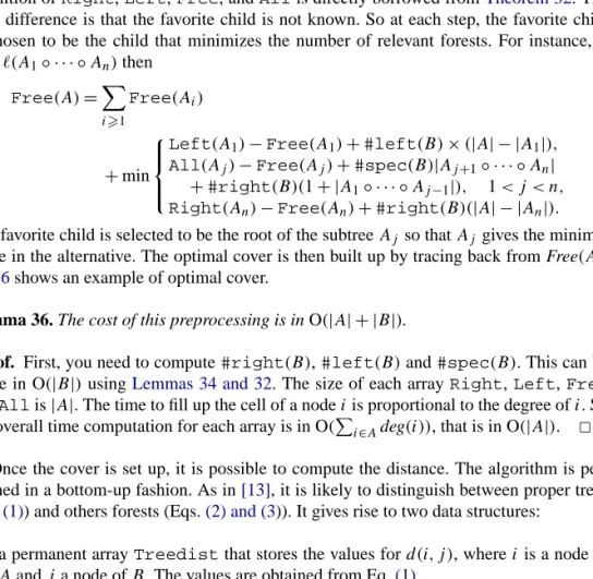
Fig. 5depicts an example of all relevant forests for a pair of trees provided with a cover strategy.
5. A new optimal cover strategy
In this last section, we show that Theorem 32makes it possible to design an optimal cover strategy. An optimal cover strategy is a strategy that minimizes the total number of relevant forests. The algorithm is as follows. For any pair of trees(A, B), define four dynamic programming tablesRight,Left,Free, andAllindexed by nodes ofA. The definition ofRight,Left,Free, andAllis directly borrowed fromTheorem 32. The only difference is that the favorite child is not known. So at each step, the favorite child is chosen to be the child that minimizes the number of relevant forests. For instance, if
A=(A1◦ · · · ◦An)then Free(A)= i1 Free(Ai) +min
Left(A1)−Free(A1)+#left(B)×(|A| − |A1|), All(Aj)−Free(Aj)+#spec(B)|Aj+1◦ · · · ◦An|
+#right(B)(1+ |A1◦ · · · ◦Aj−1|), 1< j < n, Right(An)−Free(An)+#right(B)(|A| − |An|). The favorite child is selected to be the root of the subtreeAj so thatAj gives the minimal value in the alternative. The optimal cover is then built up by tracing back from Free(A). Fig. 6shows an example of optimal cover.
Lemma 36. The cost of this preprocessing is in O(|A| + |B|).
Proof. First, you need to compute#right(B),#left(B)and#spec(B). This can be made in O(|B|)usingLemmas 34 and 32. The size of each arrayRight,Left,Free andAllis|A|. The time to fill up the cell of a nodeiis proportional to the degree ofi. So the overall time computation for each array is in O(i∈Adeg(i)), that is in O(|A|). 2
Once the cover is set up, it is possible to compute the distance. The algorithm is per-formed in a bottom-up fashion. As in[13], it is likely to distinguish between proper trees (Eq.(1)) and others forests (Eqs.(2) and (3)). It gives rise to two data structures:
• a permanent arrayTreedistthat stores the values ford(i, j ), whereiis a node of
Fig. 5. Set of all relevant forests for the pair of trees(A, B). The treeAis the cover tree. The favorite child of 1 is 3, the direction of 2 is right, the direction of 4 is left. We display all relevant forests forAandB. The three blocks forAare the three categories(α),(β)and(γ ). For each subgroup ofA, we indicate the corresponding relevant forests ofB:B#right(B)=5,#left(B)=6 (Lemma 34) and#spec(B)=6 (Lemma 35). This gives 33 pairs of relevant forests for the pair(A, B). This result is consistent withTheorem 32: the number of relevant forests is given by Free(A), and applying case 7, we have
Free(A)=Free(2)+Free(4)+All(3)+#spec(B)×1+#right(B)×2
=#left(B)+#right(B)+#spec(B)+#spec(B)+#right(B)×2
=33.
• a temporary structureForestdist that stores the values that are attached to the computation of the current cell(i, j )ofTreedist.Forestdistis filled in using Eqs.(2), (3)and previously computed cells ofTreedist.
At first glance,Forestdistcould require cubic space, when the favorite child ofiis neither the leftmost child, nor the rightmost child. But it can be made quadratic: letkbe
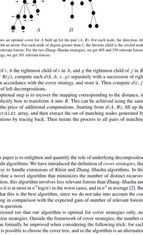
Fig. 6. This figure shows an optimal cover forAbuilt up for the pair(A, B). For each node, the direction, left or right, is indicated with an arrow. For each node of degree greater than 1, the favorite child is the circled node. This cover yields 340 relevant forests. For the two Zhang–Shasha strategies, we get 405 and 350 relevant forests, and for the Klein strategy, we get 391 relevant forests.
the favorite child ofi,hthe rightmost child ofiinA, andgthe rightmost child ofj inB. For all nodesxofB(j ), compute eachd(k..h, x..g)separately with a succession of right decompositions, in accordance with the cover strategy, and store it. Then computed(i, j )
with a succession of left decompositions.
The final and optional step is to recover the mapping corresponding to the distance, in order to know explicitly how to transformAintoB. This can be achieved using the same space amount, at the price of additional computations. Starting fromd(A, B), fill up the associatedForestdistarray, and then extract the set of matching nodes generated by replacement operations by tracing back. Then iterate the process to all pairs of matching subtrees.
6. Discussion
The goal of this paper is to enlighten and quantify the role of underlying decomposition strategies in tree edit algorithms. We have introduced the definition of cover strategies, that are natural and easy to handle extensions of Klein and Zhang–Shasha algorithms. In this framework, we define a novel algorithm that minimizes the number of distinct recursive calls. By construction, this algorithm involves less relevant forests than Zhang–Shasha and Klein strategies. So it is at most inn3log(n)in the worst cases, and inn3in average[2]. But we do not claim that this is the best algorithm, since we do not take into account the cost of the preprocessing in comparison with the expected gain of number of relevant forests. This is still an open question.
It should be stressed too that our algorithm is optimal for cover strategies only, not for all decomposition strategies. Outside the framework of cover strategies, the number of relevant forests can formally be improved when considering the following trick: for each pair of subtrees, it is possible to choose the cover tree, and so the algorithm is an alternation of cover strategies each time you compute a newForestdistarray. Unfortunately the implementation becomes much more intricate, and the gain is poor.
Finally, in this paper, we have chosen to focus on the total number of relevant forests. It is possible to develop a analogous analysis for alternative criteria. Some examples are
• minimizing the total number of forests in the temporaryForestdistarrays
• minimizing the amount of space forForestdistarrays, that is minimizing the size of the largestforestdistarray.
The technical details are very close to those described here, and most of our lemmas could be simply adapted to achieve this aim.
References
[1] S. Chawathe, Comparing hierarchical data in external memory, in: Proceedings of the Twenty-Fifth Interna-tional Conference on Very Large Data Bases, 1999, pp. 90–101.
[2] S. Dulucq, L. Tichit, RNA secondary structure comparison: exact analysis of the Zhang–Shasha tree edit algorithm, Theoret. Comput. Sci. 306 (1–3) (2003) 471–484.
[3] D. Harel, R.E. Tarjan, Fats algorithms for finding nearest common ancestors, SIAM J. Comput. 13 (2) (1984) 338–355.
[4] T. Jiang, L. Wang, K. Zhang, Alignment of trees—an alternative to tree edit, Theor. Comput. Sci. 143 (1995). [5] P. Klein, Computing the edit-distance between unrooted ordered trees, in: Proceedings of 6th European
Symposium on Algorithms, 1998, pp. 91–102.
[6] S.B. Needleman, C.D. Wunsh, A general method applicable to the search for similarities in the amino acid sequence of two proteins, J. Molecular Biol. 48 (1970) 443–453.
[7] S.M. Selkow, The tree-to-tree editing problem, Inform. Process. Lett. 6 (1977) 184–186.
[8] B. Shapiro, K. Zhang, Comparing multiple RNA secondary structures using tree comparisons, Comput. Appl. Biosci. 4 (3) (1988) 387–393.
[9] K.C. Tai, The tre-to-tree correction problem, J. ACM 26 (1979) 422–433.
[10] H. Touzet, Tree edit distance with gaps, Inform. Process. Lett. 85 (3) (2003) 123–129. [11] G. Valiente, Algorithms on Trees and Graphs, Springer-Verlag, 2002.
[12] R.A. Wagner, M.J. Fischer, The string-to-string correction problem, J. ACM 21 (1) (1974) 168–173. [13] K. Zhang, D. Shasha, Simple fast algorithms for the editing distance between trees and related problems,
SIAM J. Comput. 18 (6) (1989) 1245–1262.
[14] K. Zhang, Algorithms for the constrained editing problem between ordered labeled trees and related prob-lems, Pattern Recognition 28 (1995) 463–474.