SARIMA Model for Malaria Admission Cases for Children Less
Than Five Years in Kakamega County Referral Hospital
Patrick Theuri Berengu1*, Robert Muriungi Gitunga2 ,Kennedy Nyongesa3
1*Department of Mathematics, School of Pure and Applied Sciences, Meru University of Science and Technology-Kenya, P.O Box 972-60200 Meru, Kenya
2Department of Mathematics, School of Pure and Applied Sciences, Meru University of Science and Technology-Kenya
3Department of Mathematics, Masinde Muliro University of Science and Technology-Kenya *Email of the corresponding author: patrickberengu@yahoo.com
Abstract
According to (MOH, 2016), malaria has become a killer disease to children in Kakamega County. Children less than five years are the most vulnerable to malaria. Lack of forecasting using available data on malaria indicators hinders the monitoring and control of the disease. This study therefore sought to formulate Seasonal Auto Regressive Integrated Moving Average (SARIMA) model for malaria admission cases for children less than five years in Kakamega County Referral Hospital. The objectives of the study were; to derive SARIMA model for forecasting malaria case admission for children less than five years and to use the derived SARIMA model to forecast malaria admission cases for children less than five years. Box Jenkins Methodology was used to derive SARIMA model. The appropriate model was SARIMA (0,2,2)(0,2,2)12. The study recommends this model to be used for planning and designing an effective control strategy for this category of children at the County level. Keywords: SARIMA model, Box Jenkins Methodology, Forecasting, Malaria admission cases.
DOI: 10.7176/MTM/9-7-06 Publication date: July 31st 2019
1. Introduction
In this section background of the study has been discussed in terms of malaria burden as a whole and the challenges faced in order to reduce malaria cases especially for children less than five years. It also highlights the statement of the problem and the study objectives. It further discusses literature review.
1.1 Background of the Study
WHO (2016) estimates that 3.2 billion people are at risk of malaria worldwide and that Sub-Saharan Africa (SSA) is disproportionally affected since in 2015, the region had 88 percent of malaria cases and 90 percent of malaria deaths. WHO also estimate that the disease is a major public health problem in Africa with 191 million clinical cases. Malaria presents a major socio-economic challenge to African countries considering that Africa is the most affected region. This challenge cannot go unnoticed given that good health is not only a basic human need, but also a fundamental human right and a prerequisite for economic growth UN(2015).
Malaria is a major cause of morbidity and mortality worldwide and it mostly affects pregnant women and children less than five years of age. SSA is mostly affected with almost 86 percent of deaths occurring in children less than five years of age (WHO, 2016). Pregnant women and children are more vulnerable to malaria infection since it reduces a woman’s immunity making them more prone to infection and this puts the life of unborn baby at risk (WHO, 2016).
In Kenya, malaria remains a major cause of morbidity and mortality with more than 70 percent of the population at risk of the disease (MOH, 2016). The malaria burden in Kenya is not homogenous. The areas around the coast and western region present the highest risk, and children less than five years and pregnant women are the most vulnerable to infection. Its effects are far reaching as it also affects the economy as a whole. For instance, 170 million work days are lost each year due to the disease while 4-10 million school days are lost by children (Tilson,2018). Its therefore not only considered as a health issue but also a socio-economic burden by the Kenyan government and therefore investment in its control should be a priority (MOH, 2016).
1.2 Statement of the Problem
Nationally, malaria is responsible for 30 percent of outpatient consultations, 19 percent of hospital admissions and 3-5 percent of inpatient deaths (KEMRI,2016). However, due to the heterogeneous nature of malaria
distribution in the country, the burden is much higher in some areas such as western Kenya. A survey of all registered causes of admission in hospitals in Western Kenya done by Kapesa et al (2018) found 47% of admissions were due to malaria. The disease was a major cause of admission in epidemic prone setting where 63.4% of children less than five years and 62.8% of patients greater than or equal to 5 years were admitted due to malaria (p>0.05) and 40% of all malaria admissions were school age children. Malaria related death rate was highest among children less than five years at the hyperendemic site, that is 60.9 death per 1000 malaria admissions.
The ability to predict malaria incidence accurately is a major milestone in the control and management of the disease. According to (INICEF,2015) malaria is the third leading cause of death in children under five years worldwide, after pneumonia and diarrheal diseases. This study focuses on generating Seasonal Auto Regressive Integrated Moving Average (SARIMA) model for malaria admission cases for children less than five years.
1.3 Objectives of the Study
To develop SARIMA model for malaria admission cases for children less than five years at Kakamega County Referral Hospital.
The specific objectives were;
i) To derive SARIMA Model for forecasting malaria admission cases for children less than five years in Kakamega County Referral Hospital
ii) To use the derived SARIMA model to forecast malaria admission cases for children less than five years in Kakamega County Referral Hospital.
1.4 Literature Review
Using malaria case numbers, and additional data on coverage of both preventive and curative interventions, environmental factors and patient demographics as risk factors, various models have been used to predict future malaria cases over certain periods of time in different geographical settings (Wangdi et al,2010).
The study carried out by Kumar et al (2014) used climatic factors including; mean monthly rainfall, mean maximum temperature and relative humidity, as risk factors to predict monthly malaria cases in Delhi, India. Seasonal ARIMA models were used with an ARIMA (0, 1, 1) (0, 1, 0)12 being identified as the best fit model and a stationary R-squared statistic was employed to evaluate the model’s goodness of fit. Only rainfall and relative humidity lagged at one month were found to be significant predictors of malaria cases in the study region.
The study done by Ezekie et al (2014) used SARIMA models to model and forecast malaria mortality rate in Nigeria. The data was first differenced to obtain stationarity with the model parameters being estimated through the Maximum Likelihood Method (MLE). The AIC (Akaike Information Criterion) and BIC (Bayesian Information Criterion) were used for model selection where the model with the lowest statistic being chosen as the best fit. Past malaria mortality data was used to forecast out of sample future values. A SARIMA (1, 1, 1) (0, 0, 1)12 was selected as the best model to predict malaria mortality rate given the available data in Nigeria. While developing a five year forecasting model for malaria incidence among children under the age of five in the Edum Banso sub-district of Ghana, Amedenu (2017) used Box and Jenkins ARIMA methodology to obtain the best fitting model by comparing Mean Absolute Error (MAE) and Stationary-R Square values, and Q -plots of residuals of the suggested models. Comparative analysis showed that ARIMA (1, 1, 2) had the best performance. The five year forecast showed a linear trend angled diagonally up. This means malaria cases in children under five in the Edum Banso sub-district of Ghana would increase steadily over the next five years (2013-2018). Gikungu et al (2015) used SARIMA model to forecast Kenya's inflation rate using quarterly data for the period 1981 to 2013 obtained from Kenya National Bureau of Statistics ((KNBS). SARIMA (0,1,0) (0,0,1)4 was identified as the best model. This was achieved by identifying the model with the least AIC. The parameters were then estimated through the Maximum Likelihood Estimation method.
This study therefore develops SARIMA model to be able to forecast malaria case admission for children less than five years in Kakamega County.
2. Research Methodology
2.1 Introduction
This section highlights data description in terms of data collection, stationarity and seasonality. It discusses derivation of SARIMA model using Box Jenkins Methodology and testing of normality. It finally discusses forecasting.
2.2 Data collection
The secondary data was used. This data was from Kakamega County Referral Hospital records which had been updated in District Health Information System (DHIS) for children less than five years.
2.3 Stationarity
Before searching for the best model for the data, the first condition was to check whether the series is stationary or not. This was done by examining time plot of the data, plotting mean and standard deviation, Augmented Dickey Fuller (ADF) test and by plotting ACF and PACF graphs. A time series is said to be stationary if its statistical properties such as mean, variance remain constant over time.
2.4 Seasonality
When the time series data has the seasonality component, seasonal differencing is recommended to make the data stationary. Seasonal differencing is recommended to be done before the first difference of the whole series as this might make the data stationary (Hamilton,1994). Seasonality was tested by plotting ACF graph.
2.5 Derivation of SARIMA model using Box Jenkins Methodology
This research focused in detail on the understanding of the Box-Jenkins ARIMA modeling approach and the time series methods used in the analysis and forecasting of malaria case admissions. ARIMA model can be decomposed into AR(p) and MA(q). The order of the autoregressive component is p, the order of differencing needed to achieve stationarity is d, and the order of the moving average component is q.
The AR (p) model can be expressed as follows
=𝛿+ + t (1)
= 𝛿 + +………+ + t (2)
t (3)
Or using the backshift operator:
(ß) = 𝑒𝑡 + 𝛿 (4)
Where; 𝑒𝑡 is the error term , yt= the actual value and is stationary
𝛿 = is the mean of the AR process , i (i= 1,2,..., p) are model parameters (ß) is the autoregressive operator of order p defined by
(ß) = 1 − 1(ß) − 2(ß2) − ⋯ − p (ß𝑝) . (5)
The AR (p) is a polynomial of degree p.The MA (q) model can be expressed as follows
=𝜇- + t (6)
= 𝜇 - +………- + t (7)
Or using the backshift operator:
− 𝜇 = (ß) t (9)
Where ( − 𝜇) is the white noise, 𝜇 is the mean of the time series (ß) is the moving average operator of order q defined by
(ß) = 1 − 𝜃1(ß) − 𝜃2(ß2) − ⋯ − 𝜃𝑞 (ß𝑞 ) (10)
Combining AR (p) model and The MA (q) model gives us ARMA (p, q) model which is given by
= 𝛿 + t - (11)
Or using the backshift operator:
(ß) = 𝛿 + ß (𝑒𝑡) (12)
Thus the general ARIMA model is given as
zt= - + 𝛿 + t (13)
The SARIMA model incorporates both non-seasonal and seasonal factors in a multiplicative model. The model is written as: ARIMA (p, d, q) × (P,D,Q)s where p, d, q, are the non-seasonal orders AR, differencing and MA respectively. P, D, Q, are the seasonal AR order, seasonal differencing order and seasonal MA order respectively. s=time span of repeating seasonal pattern.
Thus the SARIMA used was given by,
𝜑(𝐵)𝛷(𝐵)(1−𝐵)𝑑(1−𝐵s)𝐷𝑦𝑡 =𝜃(𝐵)𝛩(𝐵)𝜀𝑡 (14)
Where s is the number of periods per season, 𝑦𝑡 is the time series observation at time t, 𝜀𝑡 is white noise, μ is
the mean of the series, 𝛷 is seasonal AR parameters, 𝜑 is non-seasonal AR parameters, 𝛩 is the seasonal MA parameters, 𝜃 is non-seasonal MA parameters, and 𝐵 is the back shift operator.
Non-seasonal components are:
AR:φ(B)=1−𝜑1𝐵−𝜑2𝐵2−⋯ −𝜑𝑝𝐵𝑝 (15)
MA: θ(B)=1+ 𝜃1𝐵 +𝜃2𝐵2 … +𝜃𝑞𝐵𝑞 (16)
and the seasonal components are:
Seasonal AR: Φ(B)=1−𝛷1𝐵𝑆−𝛷2𝐵2𝑆−⋯ −𝛷𝑃𝐵𝑃𝑆 (17)
Seasonal MA: Θ(B)=1+ 𝛩1𝐵𝑆 +𝛩2𝐵2𝑆 … +𝛩𝑄𝐵𝑄𝑆 (18)
Various combinations of SARIMA model were generated and the one with the lowest AIC was selected.
2.6 Normality Test
The third step proposed by Box Jenkins is model diagnostics checking. Model checking is done through residual analysis. If the identified model is adequate, the residual observations should be transformed to a white noise process where the residuals are random and have the normal distribution. Normality was thus tested by generating standardized residual plot, Histogram plot, Normal Q-Q plot and correlogram plot.
2.7 Forecasting
The last step proposed by Box Jenkins is forecasting. Forecasting is the last stage after the model has been identified and fitted. The model may be used to generate forecasts of future values. Forecasting was thus done
using the generated SARIMA model. 3. Results and Discussions
3.1 Introduction
This section present results and discussion relating to data description, SARIMA model and forecasting using the generated SARIMA model.
3.2 Malaria data
The Malaria data used for analysis was available monthly as from January 2000 to March 2017.This data was used since it is a time series data. The variable of interest was malaria case admission for children less than five years
3.3 Stationarity in the data
Before searching for the best model for the data, the first condition was to check whether the series is stationary or not. The stationarity condition ensures that the autoregressive parameters in the estimated model are stable within a certain range as well as the moving average parameters in the model are invertible. If this condition is assured then, the estimated model can be forecasted [14]. A time series is said to be stationary if its statistical properties such as mean, variance remain constant over time.
3.3.1 Checking stationarity through examining time plot of the data.
Malaria data was plotted and stationarity was examined through visual inspection of time series plot to know whether the mean and standard deviation was constant or varied with time as shown in figure 1.
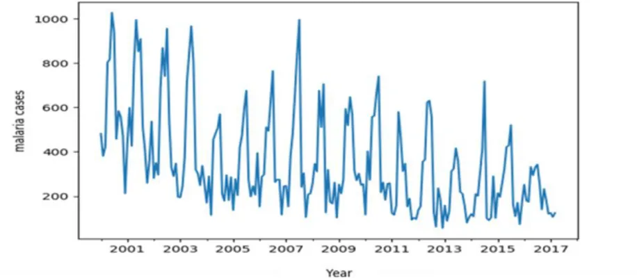
Figure 1: Malaria cases for children less than five years in Kakamega General Hospital
Kakamega County Referral Hospital malaria data was plotted and through observation, Figure 1 reveals that the data is not stationary. The graph shows there is general rise and fall of malaria cases over the years. But by critical observations year by year, it is clear that, there existed a sharp rise and fall in the malaria cases recorded. However the highest malaria case was recorded in the year 2000 and the least recorded in the year 2013. It is evident that there is an increasing and decreasing trend in the data making it non-stationary.
3.3.2 Checking stationarity through plotting mean and standard deviation
A plot of mean and standard deviation was done to check if it varied with time as shown in Figure 2.
From the Figure 2 above, where mean and standard deviation was plotted against the original data it can be seen that both mean and standard deviation varied with time making the data non- stationary.
3.3.3 Checking Stationarity through Augmented Dickey- Fuller Test
Also, unit root tests are performed on the data to confirm stationarity and to make sure that differencing is necessary. Stationarity was also tested using the Augmented Dickey–Fuller (ADF) test.
Table 1. Results of Augmented Dickey–Fuller test
Test type Test Statistic p-value
ADF -2.063612 0.259396
The null hypothesis of the test is that the time series can be represented by a unit root, that it is not stationary (has some time-dependent structure). The alternate hypothesis (rejecting the null hypothesis) is that the time series is stationary.
If p-value > 0.05: Accept the null hypothesis (H0), the data has a unit root and is non-stationary.
If p-value <= 0.05: Reject the null hypothesis (H1), the data does not have a unit root and is stationary.
The results from Table 1 indicates that p value=0.259396 and is greater than 0.05 we accept the null hypothesis and conclude that the time series data in this study is not stationary.
3.3.4 Checking Stationarity through Plotting ACF and PCF Graphs
For a stationary time series, the ACF and PACF will drop to zero relatively quickly, while the ACF and PACF of non-stationary data decreases slowly. The ACF and the PACF graphs of the data were plotted to determine whether the series is stationary or not as shown in figure 3 and 4 respectively.
Figure 3 Autocorrelation
Figure 3 shows that ACF does not drop to zero quickly but slowly thus indicating that the data is not stationary. Further it shows that after every 12th lag there is a significant spike thus indicating that the data has aspects of
seasonality.
The PACF graph in Figure 4 also does not drop to zero quickly and through observation it dies off slowly thus indicating that the data is not stationary.
3.4 Seasonality
If the series is non-stationary the series has to be either differenced to make it stationary in mean, or transformed if the covariance between any two observations 𝑌𝑡 and 𝑌𝑡+𝑖 is not constant over time. The order of differencing
denoted by d is the number of times the original series must be differenced in order to achieve stationarity.
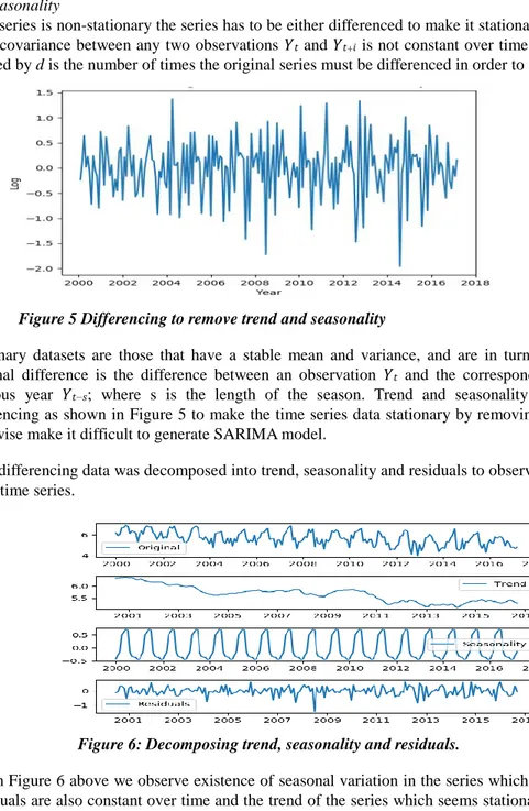
Figure 5 Differencing to remove trend and seasonality
Stationary datasets are those that have a stable mean and variance, and are in turn much easier to model. A seasonal difference is the difference between an observation 𝑌𝑡 and the corresponding observation from the
previous year 𝑌𝑡−𝑠; where s is the length of the season. Trend and seasonality were eliminated through
differencing as shown in Figure 5 to make the time series data stationary by removing the effect of time which otherwise make it difficult to generate SARIMA model.
After differencing data was decomposed into trend, seasonality and residuals to observe the various components in the time series.
Figure 6: Decomposing trend, seasonality and residuals.
From Figure 6 above we observe existence of seasonal variation in the series which is constant over time, the residuals are also constant over time and the trend of the series which seems stationary and also constant over time. The original data seems to be constant over time. From observation, seasonal effect occurred every year or every twelve month period from 2000 through to 2017.
3.5 SARIMA model
SARIMA model was identified using Box Jenkins forecasting methodology in terms of model identification and model estimation.
3.5.1 Model identification by using ACF and PACF graphs of the differenced time series
The first step according to Box Jenkins is model identification. This step involved the identification of a tentative model by establishing the number of parameters involved and their combinations. This involved determining the order of the model required (p, q) in order to capture the features of the data. This was done by plotting the ACF and PACF graphs of the differenced data.
The ACF and PACF graphs of differenced time series can be used to estimate the order of p and q. Thus these two graphs were plotted as shown in Figures 7 and 8 respectively.
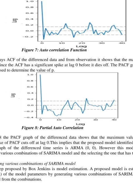
Figure 7: Auto correlation Function
Figure 7 displays ACF of the differenced data and from observation it shows that the maximum value of q for this data is 0 since the ACF has a significant spike at lag 0 before it dies off. The PACF graph of the differenced series can be used to determine the value of p.
Figure 8: Partial Auto Correlation
From Figure 8 the PACF graph of the differenced data shows that the maximum value of q is 0 since the significant spike of PACF cuts off at lag 0.This implies that the proposed model identified by checking the ACF and PACF graph of the differenced time series is ARMA (0, 0). However this model was confirmed by generating the various combinations of SARIMA model and the selecting the one that has the lowest AIC.
3.5.2 Generating various combinations of SARIMA model
The second step proposed by Box Jenkins is model estimation. A proposed model is estimated by finding the values (p, d, q) of the model parameters by generating various combinations of SARIMA models and the best model selected from the combinations.
Given a random sample X1, X2 …….. Xn for which the probability density (or mass) function of each Xi is f (xi|θ).
Then, the joint probability mass (or density) function of X1, X2, …………. Xn, which is given by f (X1, X2
…….. Xn ; θ) and its likelihood is
L(θ) =P(X1=x1,X2=x2⋯⋯,Xn=xn) = f(x1|θ)⋅f(x2|θ) ⋯⋯⋯f(xn|θ) (19)
L(θ) = (20)
Therefore MLE is the value that maximizes L(θ)
The model with the lowest AIC is usually selected as the best fit. These information criterion judges a model by how close its fitted values tend to be to the true values, in terms of a certain expected value. The criterion value assigned to a model is only meant to rank competing models and tell you which is the best among the given alternatives.
The formula for the AIC is:
𝑊ℎ𝑒𝑟𝑒: 𝑚 is the number of model parameters (𝑚 = 𝑝 + 𝑃 + 𝑄 + 𝑞); 𝑛 is the number of observations, or equivalently, the sample size
Various combinations of ARIMA models were generated with the corresponding AICs as follows; ARIMA(0, 1, 2)x(0, 2, 2, 12)12 – AIC:1952.80539227 ARIMA(0, 2, 2)x(0, 2, 2, 12)12 – AIC:1944.19072277 ARIMA(0, 2, 2)x(1, 2, 2, 12)12 – AIC:1946.6745272 ARIMA(1, 0, 1)x(0, 2, 2, 12)12 – AIC:1973.36349368 ARIMA(1, 0, 2)x(1, 2, 2, 12)12 – AIC:1964.74946516 ARIMA(1, 1, 1)x(0, 2, 2, 12)12 – AIC:1964.64013208
From the results above the most suitable model for forecasting malaria cases in this study is SARIMA (0, 2, 2) x (0, 2, 2, 12) as this model has the lowest AIC value of 1944.19072277.
3.5.3 Checking normality of the data
The third step proposed by Box Jenkins is model diagnostics checking. This step involves checking model adequacy, and if necessary incorporating potential improvements. Model checking is done through residual analysis. If the identified model is adequate, the residual observations should be transformed to a white noise process where the residuals are random and have the normal distribution.
The residuals of an ARMA (p, q) can be obtained by:
+ - (22)
The residuals of the model should be randomly distributed with zero-mean and not serially correlate, i.e to be white noise. If the fitted seasonal ARIMA model does not satisfy these properties, it is a good indication that it can be further improved.
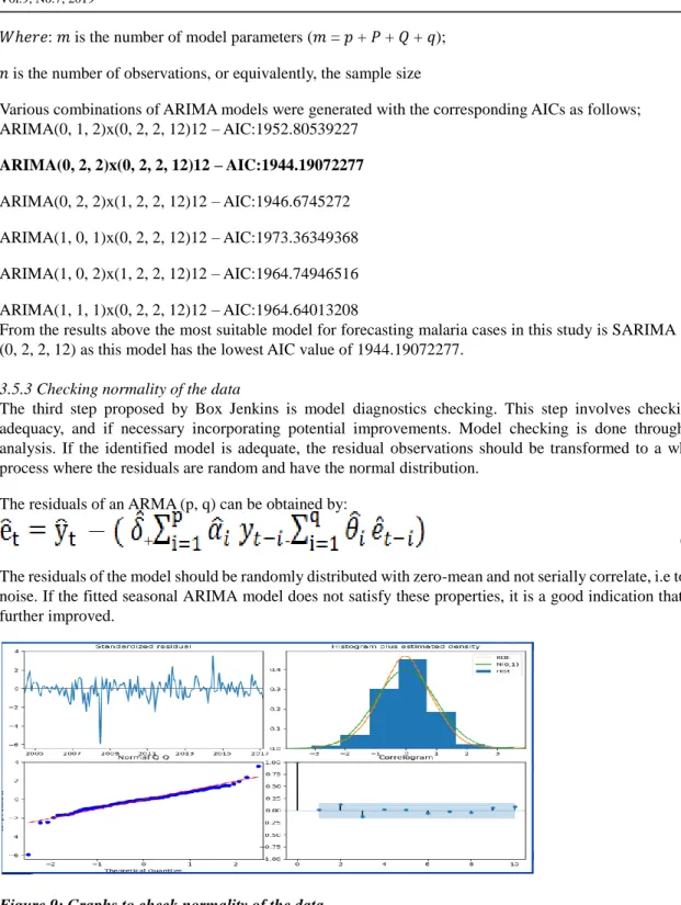
Figure 9: Graphs to check normality of the data
From Figure 9 the residual plot of the fitted model in the upper right corner and appears to be white noise as it does not display obvious seasonality or trend behavior. The plot also shows that the residuals have zero mean, constant variance and also uncorrelated. The histogram plot in the upper right corner pair with the kernel density estimation (red line) indicates that the time series is almost normally distributed since it portrays a bell shaped distribution which is associated with a normal distribution. This is compared to the density of the standard normal distribution (green line). The correlogram (autocorrelation plot) confirms these results, since the time series residuals show low correlations with lagged residuals. Q-Q plots display the observed values against normally distributed data represented by the red line. Most of the points pass through the straight red line with few of the points very close to this straight line. This shows that the residuals in the model are normal. This makes the SARIMA (0, 2, 2) x (0, 2, 2, 12) to be the best model in this study.
3.6 Forecasting
The last step proposed by Box Jenkins is forecasting. The model may be used to generate forecasts of future values. The current time is denoted by t, the forecast for y𝑡+𝑘 is the k-period- ahead forecast is denoted
by .
For an ARIMA (p, d, q) process at time 𝑡 + 𝑘 (k periods in the future) the model is:
+ + - (23)
Using the backshift operator the proposed ARIMA model that describes the data is given by (1- B)2 (1- B 12)2y
t= (1+ 1 B + 2 B 2) (1+ Θ1B12+ Θ2 B24)et (24)
which after expansion results to
yt = et+ Θ1 et-12 + Θ2 et-24 + 1et-1 + 1 Θ1 et-13 + 1 Θ2 et-25 + 2et-2+ 2 Θ1 et-14 + 2 Θ2 et-26 (25)
where 1= -2.21 2=1.21 Θ1=1.97 Θ2 =1.00
Replacing the coefficients we have the forecasting model as
yt = et-1.97 et-12+ et-24 -2.21 et-1+4.35 et-13-2.21 et-25+1.21 et-2-2.38 et-14+1.21 et-26 (26)
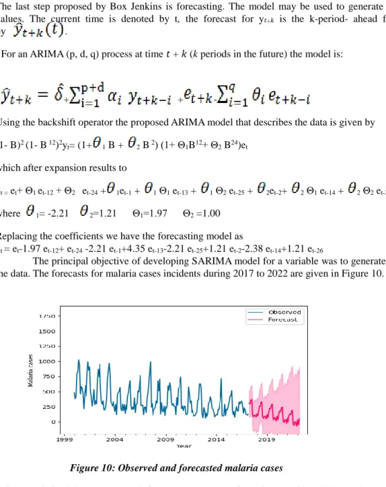
The principal objective of developing SARIMA model for a variable was to generate forecasts based on the data. The forecasts for malaria cases incidents during 2017 to 2022 are given in Figure 10.
Figure 10: Observed and forecasted malaria cases
Using the derived SARIMA model, forecasts were made from the year 2017-2022 as shown in Figure 10 which shows a slow decrease in malaria cases from the year 2017-2022.
4. Conclusions and Recommendations
4.1 Introduction
From the forecasted SARIMA model generated the following conclusion and recommendations were drawn.
4.2 Conclusion
National control and prevention strategies will be greatly enhanced through better ability to forecast future trends in the disease incidence. SARIMA (0, 2, 2)(0,2,2 12) model generated provides the means to better understand malaria dynamics thereby yielding forecast that can be used for public health planning, designing an effective prevention and control strategy for malaria cases at the County level. The monthly malaria incidence record of children less than five years in Kakamega County Referral Hospital has been studied using the Box-Jenkins (ARIMA) model methodology and the model predicts slow decrease in malaria incidences in the period 2017-2022.
4.3 Recommendations
It is recommended that the government use the formulated model to predict malaria incidences and enable them administer adequate and timely malaria control and preventive measures to the Kakamega County Referral Hospital.
The study also recommends to Kakamega County Referral Hospital management staff to ensure that the hospital has sufficient and effective malaria drugs, sufficient pediatric beds and screening equipments to enable them respond to malaria cases for children less than five years that are reported at the hospital.
References
Amedenu.S.B.(2017). Nonseasonal ARIMA Modeling and Forecasting of Malaria Cases in Children under Five in Edum Banso Sub-district of Ghana .Asian Research Journal of Mathemtics,4(3),1-11.
Ezekie D, Opara, J. & Idochi, O (2014): Modeling and Forecasting Malaria Mortality Rateusing SARIMA Models (A Case Study of Aboh Mbaise General Hospital, Imo State Nigeria). Science Journal of Applied
Mathematics and Statistics,2(1),31-41.
Gikungu.S.W., Anthony G. Waititu, Kihoro.J.M.,Waititu.A.G (2015). Forecasting Inflation Rate in Kenya Using SARIMA Model. American Journal of Theoretical and Applied Statistics.,4 (1), 15-18.
Hamilton, J. D. (1994). Time Series Analysis. Princeton Univ. Press, Princeton New Jersey.
Kapesa A, Kweka EJ, Atieli H, Afrane YA, Kamugisha E (2018) The current malaria morbidity and mortality in
different transmission settings in Western Kenya. PLOS ONE 13(8):
e0202031. https://doi.org/10.1371/journal.pone.0202031
KEMRI (2016). The US Centers for Disease Control and Prevention and Liverpool School of Tropical Medicine report .Retrieved from https://www.kemri.org
Kumar V, Mangal, A, Panestar, S., (2014): Forecasting Malaria Cases Using Climatic Factors in Delhi, India: A Time Series Analysis. Malaria Research and Treatment 3(1)1-6.
Ministry of Helth (2016). Kenya Malaria Indicator Survey 2015. Retrieved from www.knbs.or.ke/kenya malaria indicator survey-2015/
Tilson, D (2018):Factors Affecting Use of Insecticide Treated Nets by Children Under Five Years of Age in Kenya. American Journal of Health Research ; 6(4),3.
United Nations (2015). The Sustainable Development Goals Report. Retrieved from
https://unstats.un.org/sdgs/files
UNICEF (2015): Malaria and children: Progress in Intervention Coverage. Pp; 69.
Wangdi K, Singhasivanon P, Silawan T, Lawpoolsri S, White NJ & Kaewkungwal J (2010): Development of temporal modeling for forecasting and prediction of malaria infections using time-series and ARIMAX analyses: A case study in endemic districts of Bhutan, 3(9).